O
pen
A
rchive
T
OULOUSE
A
rchive
O
uverte (
OATAO
)
OATAO is an open access repository that collects the work of Toulouse researchers and
makes it freely available over the web where possible.
This is an author-deposited version published in :
http://oatao.univ-toulouse.fr/
Eprints ID : 18142
To link to this article : DOI:10.1021/acs.iecr.6b03627
URL :
http://dx.doi.org/10.1021/acs.iecr.6b03627
To cite this version :Bernard, Manuel and Climent, Eric and Wachs,
Anthony Controlling the Quality of Two-Way Euler/Lagrange
Numerical Modeling of Bubbling and Spouted Fluidized Beds
Dynamics. (2017) Industrial & Engineering Chemistry Research, vol.
56 (n° 1). pp. 368-386. ISSN 0888-5885
Any correspondence concerning this service should be sent to the repository
administrator:
[email protected]
Controlling the Quality of Two-Way Euler/Lagrange Numerical
Modeling of Bubbling and Spouted Fluidized Beds Dynamics
Manuel Bernard,
†Eric Climent,
‡and Anthony Wachs
*
,§,∥†Fluid Mechanics Department, IFP Energies Nouvelles, 69360 Solaize, France
‡Institut de Mécanique des Fluides de Toulouse, Université de Toulouse - CNRS, INPT, UPS - 31400 Toulouse, France
§Department of Mathematics, University of British Columbia, 1984 Mathematics Road, Vancouver, BC, Canada V6T 1Z2
∥Department of Chemical & Biological Engineering, University of British Columbia, 2360 East Mall, Vancouver, BC, Canada
V6T 1Z3
ABSTRACT: We numerically simulate three-dimensional fluidized beds of monodisperse spheres using a two-way Euler/Lagrange method. Particles trajectories are tracked in a Lagrangian way, and particles collisions are computed by a soft
sphere model. Thefluid conservation equations are written in
a classical Eulerian fashion and are locally averaged on cells 1 order of magnitude larger than particles. We detail the equations of the model and their numerical implementation.
We study the influence of numerical parameters and
simula-tion domain size on computed results in a biperiodicfluidized
bed. We then validate the model against theoretical results for a bubbling fluidized bed and against experimental data for a
single- and multi-nozzle spouted bed. Finally, we investigate the influence of the Coulomb friction coefficient magnitude on a
single-nozzle spouted bed dynamics in order to emphasize the importance of tangential friction in such processes.
1. INTRODUCTION
Fluid−particle two-phase flows such as fluidized beds are
involved in several industrial domains as, e.g., chemical and process engineering. In fact, due to its high heat and mass
transfer rates, the fluidized bed flow configuration is widely
used in coal gasification, chemical looping combustion (CLC),
atmospheric or pressurized fluidized bed combustion (FBC),
and fluid catalytic cracking (FCC). Solid particle diameters
generally range from a few tens of micrometers to a few millimeters. Influidized or fixed beds, a lighter fluid, that can be either a liquid or a gas, is injected at the bottom wall of the reactor andflows out at the top wall of the reactor. If the force
exerted on particles by the fluid flow is strong enough (and
actually stronger than the net weight of particles), particles are fluidized, i.e., they are set in motion. In a reactor containing up to several billions of particles, their spatial distribution is very often heterogeneous. Indeed, particles trajectories are affected
both by hydrodynamic interactions with the surroundingfluid
flow and collisions with neighboring particles and wall boundaries. This leads to the formation of particles clusters
and void areas called fluid bubbles. The typical size of these
structures can be significantly larger than the average particle diameter.1−3As a result of this intricate dynamics of thefluid− particle system, the whole bed expands until it reaches a
pseudosteady state over which its height fluctuates either
slightly or markedly depending on the flow regime. This
dynamics offluidized beds is undoubtedly multiscale, from the
microscale of the fluid flow around individual particles and
interparticle contacts to the mesoscale of particle clusters and
fluid bubbles, and eventually to the macro-scale of the whole bed behavior. Related to these three spatial scales, three corresponding modeling strategies are often adopted. At the
microscale, Navier−Stokes equations are solved over the fluid
domain on a grid much thinner than each individual particle and particles trajectories are fully described. This approach
enables one to accurately compute theflow kinematics around
each solid particle. Thefluid−solid interaction is then reliably
computed by any appropriate integration of the fluid stress
tensor over the particle surface. The corresponding simulations
are high-fidelity provided the fluid cell size over particle
diameter ratio is small enough (at least 1/10 and sometimes up to 1/40 to guarantee accurate computed solutions). The aftermath of this constraint on the grid size is the rather limited size of systems that can be reasonably simulated even with massively parallel codes on the most powerful supercomputers.
Apart from a few exceptions,4 microscale simulations are
generally limited to a few thousands of particles. At the
macro-scale, both thefluid and solid phases are described by locally
averaged continuous conservation equations. Since the solid phase is assumed to be continuous, particles trajectories are not individually tracked anymore, and instead, the solid phase is described in terms of a local volume fraction or porosity. This
has been widely applied tofluidized beds by Gidaspow (see the
Two Fluid Model (TFM) in, e.g., ref5) and enables one to
examine systems containing billions of particles representative of a human-size chemical process. The mesoscale model repre-sents a compromise between microscale models and macroscale models. In the mesoscale model, often called two-way Euler/
Lagrange orDEM-CFD(for DEM (Discrete Element
Method)-CFD (Computational Fluid Dynamics)), the fluid phase is
locally averaged as in the macroscale model, but particles are still tracked individually as in the microscale model. Particle− particle and particle−wall collisions are precisely handled while fluid−solid interactions rely on closure laws. However, fluid− solid interactions are deemed to be more accurately modeled
than in macroscale Euler−Euler approaches. This results in a
better prediction of the dynamics offluid bubbles and particles clusters comprising several thousands of particles or more.
Conceptually, fluid cells in the mesoscale model are much
smaller than in the macroscale Euler−Euler model but much larger than in the microscale model. Furthermore, several numerical knacks were developed over the past 20 years to improve computing performances in such a way that nowadays simulations with up to a few tens of millions or even a few hundreds of millions of particles are attainable.6 Typically, a system containing such a number of particles mimics pretty
well a small size 3D experimentalfluidized bed and hence offers
the opportunity to perform a direct simulations−experiments
comparison. It is particularly important to emphasize that
the dynamics of afluidized bed is fully three-dimensional and
that consequently the attempt to model and understand the global behavior of a bed with 2D simulations is mostly worth-less.6
The two-way Euler−Lagrange approach has been first
introduced by Tsuji et al.7in the early 1990s. In the pioneering form of the model, collisions were handled by a soft sphere
approach. A couple of years later, Hoomans et al.8proposed a
DEM-CFD model based on a hard sphere principle. Such a
col-lision approach is better suited to dilutefluid/particles mixture since collisions are assumed to be binary and instantaneous and
therefore request to be treated one after another.9 Then, the
formulation of the model was improved by several research groups. In particular, the interested reader will refer to the
prolific scientific exchange between the group of Xu and Yu and
Hoomans and his collaborators10−12on the consistency of the model.
The total hydrodynamic force, i.e., integration offluid stress tensor over particle surface can be expressed as the sum of
different hydrodynamic contributions, mainly drag force, lift
force, added mass force, and Basset force. For gas-particles flows, the drag force is the leading contribution, and cor-respondingly, the other contributions are generally neglected. The expression of the drag force experienced by an isolated
particle in an infinite domain is well known and was derived
theoretically and empirically for Stokes and inertial flows,
respectively. This force is not only dependent on the relative
velocity between the fluid and the particle but also on the
presence of surrounding particles. The influence of surrounding particles is often expressed by the localfluid volume fraction, .f So far, there exists neither a theoretical formula nor accurate correlation that describes faithfully the drag force intensity in
moderately dense to dense suspensions and anyflow regimes.
However, several expressions were proposed in the literature with various domains of validity in terms of particle Reynolds
number Repandfluid volume fraction, . In af fluidized bed, the
solid concentration varies from close packing ( −1 ,f ≈0.6) to dilute regime (1−,f ≲0) in relation to thefluid bubbles/ particles clusters dynamics. Hence, the drag force correlation is
required to be reliable on a wide range of , . The classicalf
approach to construct such a reliable closure law is to combine
Wen and Yu’s correlation13 for dilute regimes to Ergun’s
correlation14 for dense regimes. The former is derived by
multiplying an infinitely dilute drag force formula by a function
of, while the latter is based on a porous media assumption.f
The threshold to switch from Wen and Yu’s correlation to
Ergun’s correlation and vice versa is generally set to,f = 0.8. Over the years, many other correlations were suggested in the literature. For instance, to extend the range of validity of Wen and Yu’s correlation to the full, range, Di Felicef 15
suggested an improvement based on experimental results that has been
widely adopted by the community. In Wen and Yu’s
correlation, the presence of surrounding particles is accounted for by a constant power of, . In Di Felicef ’s improved model,
the power of, is not a constant anymore but a function of Ref p
and , itself. For many years, experiments were the mostf
reliable source of data (assuming measurement uncertainty is controlled) to derive drag force closure laws. However, mea-surement techniques can be intrusive, and detailed
informa-tion in the core of the flow in a (generally fixed) bed is not
necessarily easy to extract. A more recent alternative is micro-scale simulation that supplies detailed information to derive new drag force correlations. As an example, Hill and Koch performed many lattice-Boltzmann microscale simulations on a wide range of, and suggested two drag force correlations, thef
former for low Reynolds number flows16 and the latter for
moderate Reynolds number flows.17 These two correlations
have then been employed by several other research teams. The correlations were even further improved by the group of Kuipers that suggested another correlation18also often used in the community.6,19,20
The aim of this paper is not to derive yet another drag law correlation. Our goal is to discuss the numerical implementa-tion of ourDEM-CFDmodel and examine the influence of various
numerical and geometric parameters on the computed results produced by such a numerical model. Looking at the broad literature onDEM-CFDsimulations, our impression is that many
papers do not detail enough their numerical implementation and the selected values of the associated numerical parameters. This inevitably leads to significant variations of bed dynamics
and impedes a proper comparison between different works.
From a physical viewpoint, the influence of tangential friction
onfluidized bed dynamics has not yet received a large amount
of attention, and we intend with this work to contribute to filling that gap in the literature.
The rest of the paper is organized as follows.Section 2gives
the set of volume-averaged Navier−Stokes equations describing
thefluid phase, the DEM/soft sphere model used to compute
collisions, and the interphase coupling terms. We present the numerical implementation of the model and dedicate particular
attention to the Lagrangian−Eulerian projection operator used
for interphase coupling. Using statistical analysis tools, we
investigate in Section 3the dependence of bubbling fluidized
bed dynamics to the following numerical parameters: solid
size to particle diameter ratio, and to the size of the domain in the biperiodic configuration adopted. InSection 4, we perform validation tests on two different fluidized bed configurations, a bubblingfluidized bed and a semi-3D spouted fluidized bed, i.e., a spouted bed whose depth spans a few particle diameters only, to further assess the consistency of the model and the validity
of the implementation. Finally, we perform inSection 5
sim-ulations of the same semi-3D spouted bed with different values
of the Coulomb friction coefficient to investigate the
quantitative impact of tangential friction on the dynamics of the spouted bed. A conclusion together with perspectives is given inSection 6.
2. EQUATIONS OF THE MODEL
We present below the governing equations of the model, i.e., conservation equations and closure laws, and detail their
numerical implementation. The surroundingfluid is assumed to
be Newtonian with viscosity μf and to have a constant
den-sityρf.
2.1. Computational Fluid Dynamics. In a way similar to
the TFM, thefluid phase is governed by the volume-averaged
Navier−Stokes equations. Control volumes ΔV are at least
an order of magnitude larger than the particle volume Vp.
The mass and momentum equations are solved on the
actual volume occupied by the fluid. This leads to the
clas-sical , -weighted formulation of the mass and momentumf
equations as follows: τ ε ρ ε ρ ρ ε ρ ε ε ∂ ∂ + ∇· = ∂ ∂ + ∇· = −∇ + + ∇· ⎧ ⎨ ⎪⎪ ⎩ ⎪ ⎪ u u u u F t t p ( ) ( ) 0 (1a) ( ) ( ) ( ) (1b) f f f f f f f f f f f f pf f f
where uf denotes thefluid velocity. The momentum equation
(eq 1b) does not contain any gravity term, and hence, the pressure p represents the hydrodynamic pressure, i.e., the total pressure minus the hydrostatic pressure contribution. Con-sequently, the buoyancy force exerted on particles is explicitly
accounted for in Newton’s equations such that particles are
subjected to the right net weight (Section 2.2). At the micro-scale, the stress tensorτfof an incompressible Newtonianfluid
reads as follows:
τf =μf(∇uf + ∇uft)=2μfD (2)
where D= 1(∇uf + ∇uft)
2 is the rate-of-strain tensor. Here,
Fpf represents the particles to fluid interphase momentum
transfer. The pressure gradient is not multiplied by εf in the momentum equation (eq 1b); thus, this set of equations
corresponds to the so-called model B in the literature.5 An
alternative formulation of the model is the so-called model A
in which the pressure gradient is also weighted by εf. These
two formulations lead to slightly different expressions for the interphase momentum transfer (with or without an explicit contribution of the pressure gradient). Both formulations are self-consistent and have led to long discussions in the literature (see, e.g.,refs 10−12, 21−23). There are no significant
dif-ferences in the performance of the two model formulations,21
although some authors favored model B as more prone to yield accurate results at lowfluidization velocity.12In this work, we use model B.
As fluid density ρf andfluid viscosity μf are assumed to be
constant, the system of eqs 1 can be rewritten as follows:
ε ε ρ ε ε μ ε ∂ ∂ + ∇· = ∂ ∂ + ∇· = −∇ + + ∇· ⎜ ⎟ ⎧ ⎨ ⎪ ⎪ ⎩ ⎪ ⎪ ⎛⎝ ⎞⎠ u u u u F D t t p ( ) 0 (3a) ( ) ( ) 2 ( ) (3b) f f f f f f f f f pf f f
We discretize eqs 3 with a classical Finite Volume/Staggered
Grid scheme on a Cartesian grid. Pressure and fluid volume
fraction are located at the center of each computational fluid
cell. Fluid velocity components are defined at cell face centers as follows: uiis defined at the center of the cell face
perpendic-ular to xi, i = 1, 2, 3. The system of eqs 3 is solved in time by a first-order Marchuk−Yanenko operator-splitting solution algo-rithm24,25in the spirit of a pseudo-L2projection method.
Intro-ducing a constant time stepΔtfand knowing the solution at time
tn= nΔt
fand tn−1= (n−1) Δtf, the solution at time tn+1= (n+1)
Δtfis obtained through the following sequence of subproblems:
1. Wefirst solve the following advection-diffusion problem:
ρ ε ε μ ε ρ ε * − Δ − ∇· * = − − ∇· − − u u D u F u u t 2 ( ( )) ( ) f fn f fn fn f f f n f pfn f fn fn fn 1 1 (4)
where uf*stands for the velocityfield at the intermediate
stage. Note that in eq 4, the viscous term 2 μf ∇·(εfn
D(uf*)) is treated implicitly and the explicit treatment of
the advection termρf∇·(εfn−1ufnufn) requires us to satisfy
a CFL stability condition.
2. We then impose mass conservation through the solution of a Stokes-like problem as follows:
ρ ε ε ε ε ε − * Δ = −∇ − Δ + ∇· = + + − + ⎧ ⎨ ⎪ ⎪⎪ ⎩ ⎪ ⎪⎪ u u u t p t (5a) ( ) 0 (5b) f f n f n f n f f n f n f n f fn nf 1 1 1 1
In eq 44, the viscous term 2 μf ∇ · (εfn D(u f
*)) and the
advection termρf∇ · (εfn−1ufnufn) are discretized in space with a
classical second order accurate centered scheme and a second order accurate TVD/Superbee limiter scheme, respectively (see
ref26among others).
2.2. Discrete Element Model. In DEM modeling, particles position and velocity are known for each individual particle and
particles are tracked in a Lagrangian way.27 In this work, we
assume that all particles are spherical. The linear and angular
motion of a (spherical) particle is given by the Newton’s
second law as follows:
ω = + + = + ⎧ ⎨ ⎪ ⎪ ⎩ ⎪ ⎪ v g f f I T T m d dt m d dt (6a) (6b) p p p pp fp p p pp fp
where mp=ρpπdp3/6 is the particle mass,ρpthe particle density,
dpthe particle diameter, Ip= ipIthe particle moment of inertia tensor, I the identity tensor, ip = ρp πdp5/60 the diagonal
coefficient of Ip, g the gravity acceleration, vp the particle translational velocity, andωpthe particle angular velocity. Here,
fppis the total particle−particle and wall−particle contact (also denoted as collision) force acting on the particle, and ff pis the
total fluid−particle hydrodynamic interaction force. Also Tpp
hydro-dynamic torque, respectively. To solve the system of eqs 6, we need a model for the contact contribution (fpp,Tpp) as well as a
model for the hydrodyamic contribution (ff p,Tf p).
The binary hard sphere model and soft sphere model are the two categories of collision models generally used for
particu-late flows.28For the former, the whole momentum exchange
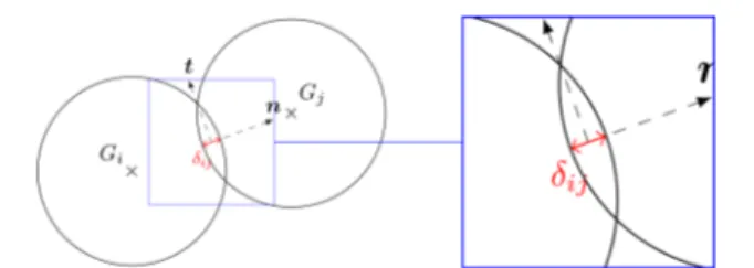
between two colliding particles takes place exactly at the time when the two particles touch each other. Thus, contacts are instantaneous, and even if a particle is colliding with more than one neighboring particle, contacts must be treated one after another, i.e., in a binary way. In contrast, for the latter, particles overlap slightly (Figure 1) such that a contact lasts a few time
steps and that collision forces are function of overlap distance δijand relative velocity vrbetween two colliding particles. Then,
contacts between a given particle and its colliding neighbors can be integrated in time all together.
In our DEM granular solver,29,30 the total collision force comprises the following terms:
• An elastic restoring force δ
=
fel kn ij ijn (7)
in the normal direction where kn denotes the normal
contact stiffness, δij the overlapping distance between
particles i and j, and nijthe unit normal vector between particles i and j centers of mass.
• A viscous dynamic force γ
= −
fdn 2n ij rn ijmv , (8)
in the normal direction to account for the dissipative
nature of the contact, where γn is the normal dynamic
friction coefficient,m = M M+
M M
ij
i j i j
the reduced mass of par-ticles i and j, and vrn,ij the normal relative velocity
between particles i and j. • A tangential friction force
μ = − | | | | ft min{ C elf , fdt }tij (9) γ = − fdt 2tmij rt ijv , (10)
where fdtdenotes the dissipative frictional contribution,γt
the dissipative tangential friction coefficient, vrn,ij the tangential relative velocity between particles i and j, and tijthe unit tangential vector. Note that the magnitude of the tangential friction force is limited by the Coulomb frictional limit calculated with the Coulomb dynamic friction coefficient μC.
The total collision force acting on a particle i is the sum of contributions related to the contact with neighboring particles j and walls w:
∑
∑
∑
∑
= + = + + + + + f f f f f f f f f ( ) ( ) pp i j pp ij w pp iw j el dn t ij w el dn t iw , , , (11)Since for a sphere the radial vector Rijfrom particle i center of
mass to the point of contact with particle j is always colinear to the unit normal vector nij, only the tangential contact force
contributes to the contact torque (same applies for a contact with a wall). The corresponding total collision torque for spheres hence reads as follows:
∑
∑
= ∧ + ∧ Tpp i R f R f j ij t ij w iw t iw , , , (12)The Lagrangian tracking of all particles with collisions is computed by our in-house massively parallel DEM solver
Grains3D.29 In this DEM code, we solve Newton’s eqs 6 in
time with a second order time-accurate leapfrog scheme. Thus, particles linear and angular velocity (vp,ωp) and position (xp,θp) are computed in the following way:
ω ω + Δ = − Δ + ∑ Δ + Δ = − Δ + ∑ Δ v v f T t t t t t m t t t t t t i t ( /2) ( /2) ( ) ( /2) ( /2) ( ) p p p p p p p p p p p p (13) θ θ ω + Δ = + + Δ Δ + Δ = + + Δ Δ x t t x t v t t t t t t t t t ( ) ( ) ( /2) ( ) ( ) ( /2) p p p p p p p p p p p p (14)
whereΔtpdenotes the solid time step. Note that the integration
of θpas written above is only formal. In practice, it involves
rotation matrices or quaternions. Grains3D can compute col-lisions between particles of arbitrary convex shape. In fact, the
collision detection strategy is based on a Gilbert−Johnson−
Keerthi (GJK) distance algorithm.31However, for spheres, the
contact detection (contact point and overlap distance) relies on
an analytical formula (Figure 1). This remarkably speeds up
contact detection. To accelerate even more contact detection, a classical linked-cell spatial sorting32is used to identify particles that potentially collide. More details about the granular solver
Grains3D can be found in.29
2.3. Action of the Fluid on Particles. Following the
classical DEM-CFD models in the literature, we neglect the
hydrodynamic torque Tf pin eq 6b. This implies that particles
angular motion is due to collisions only. The fluid−solid
interaction force ff pderives from integration of thefluid stress
tensor over the particle surface and requires to be closed. In this study, we assume that dominant hydrodynamic forces are buoyancy force and drag force. The added mass force and the Basset force are assumed to be negligible due to the high solid/ fluid density ratio and the low fluid viscosity considered later on in this work. Finally, we neglect the Saffman lift force and the Magnus lift force for the two following primary reasons: (i) to
be coherent with the assumption Tf p= 0 as these two forces
implyfluid-induced particle rotation and (ii) the lack of reliable correlations in the literature at high solid volume fraction/low
εf (hindrance effect). Thus, the force exerted by the fluid on
each individual particle is ρ
= − +
ffp fVpg fD (15)
Figure 1.Contact between two particles: Giand Gjdenote the centers of mass of particles i and j, respectively, M the contact point, n and t the unit normal and tangential vectors at the contact point, respectively, andδijthe overlapping distance.
where−ρf Vpgcorresponds to buoyancy force and fDto drag force. Several drag force expressions have been suggested in
the literature depending on the flow regime characterized by
particle Reynolds number Repand localfluid volume fraction εf.
All these expressions can be written in the following form: β ε ε = − − f V u v (1 )( ) D p f f f p (16)
whereβ denotes the interphase momentum transfer coefficient.
The presence of 1/εfin the denominator is specific to model B.
Indeed, coefficients β in model A and model B are related to
each other by the following formula:βB= βA /εf.5 In process engineering, the most commonly used expression of this
coefficient is a combination of Wen and Yu’s equation for low
particle concentration (high εf, dilute regime) 13
to Ergun’s equation for moderate to high particle concentration (low εf, dense regime):14 β ε μ ε ε ρ = − + − |u −v| d d 150 (1 ) 1.75 (1 ) f f f p f f p f p Ergun 2 2 (17) β = C −ε ε |u −v|ε− d 3 4 (1 ) D f f p f p f Wen&Yu 2.65 (18)
where the drag coefficient CDis given by the Schiller−Naumann
correlation33as follows: = + < ⩾ ⎧ ⎨ ⎪ ⎩ ⎪ C Re Re Re Re 24 (1 0.15 ) 1000 0.44 1000 d p p p p 0.687 (19)
where the particle Reynolds number Repis defined as
ρ ε μ = |u −v| Re d p f p f f p f (20)
To avoid any discontinuity between eqs17and18, Huilin and
Gidaspow34 introduced an additional function that smoothes
out the transition from low to highεf regimes.
φ ε π = × − − + − tan (150 1.75(0.2 (1 ))) 0.5 f Huilin 1 (21)
βHuilin =(1−φHuilin)βErgun +φHuilin Wen&Yuβ (22)
Over the past 20 years, other correlations reasonably valid
for a wide range of Rep and εf were suggested in the
litera-ture.15,17,18,35 Among others, the expression proposed by Beetstra et al.18seems to perform quite well:
β μ ε ε = − + d F F 18 (1 ) ( ) f f f p Beetstra 2 1 2 (23) with ε ε ε ε = − + + − F 10(1 f) (1 1.5 1 ) f f f 1 2 2 (24) ε ε ε ε = · + − + + ε ε − − − − − F Re Re Re 0.413 24 3 (1 ) 8.4 1 10 p f f f f p p 2 2 1 0.343 3(1 f) 2.5 f (25)
In this work, simulations are performed with the expression of
Huilin and Gidaspow34or the expression of Beetstra et al.18
As plotted in Figure 2, different drag correlations predict
significantly different values of the drag force for low εf(dense regime), while they generally agree with each other for highεf
(dilute regime).
2.4. Action of Particles on the Fluid. According to
Newton’s third law of motion (action−reaction principle),
momentum transfer from solid phase tofluid phase should be
equal to the one from fluid phase to solid phase but with
opposite sign. This equality has to be satisfied at a global
level as much as at the local level, i.e., in each cell of the
computationalfluid domain. Note that for consistency with the
form of eq 1b without any gravity term, there is no contribution of the buoyancy force in the action of the particles on thefluid.
When a particle belongs to a single computationalfluid cell,
its total drag force fdcontributes to Fpf in that cell. However,
when a particle overlaps severalfluid cells, the contribution of
its drag force fdmust be shared between (projected onto) the
cells it belongs to. Here, Fpf represents a source term in the momentum equation (eq 3b) and is computed explicitly before
each fluid solver iteration. It models the particles feedback
effect or particles reaction on the fluid. Here, we use a simple projection operator based on the fraction of the particle
belonging to a control volume. Hence, Ff p is computed as
follows:
∑
θ = F f V 1 pf kCV i i k D i, , (26)where θi,kis a measure of the fraction of particle i in control volume k. The computational details to estimateθi,kare given in
Section 2.5. With the Finite Volume/Staggered Grid discretiza-tion scheme used in this study, the projecdiscretiza-tion of fdto compute
Fpfis performed for each velocity component separately as each
velocity component is defined on a different control volume
(staggered layout of the velocity components).
2.5. Projection Operator from Lagrangian to Eulerian. We detail here how we project Lagrangian quantities on the Eulerian grid and illustrate the method on the computation of
the fluid volume fraction εf. The same projection operator is
used to project the hydrodynamic Lagrangian forces fdon the
Eulerian grid to compute the source term Fpf (particles
reac-tion of thefluid) in the momentum equation. The projection
operator is a key component of the interphase coupling. For instance, the drag force acting on a particle is highly dependent
Figure 2.Drag force depending on the fluid volume fraction for a particle of diameter dp= 10−3 m with a relative velocity |uf− vp| = 0.35 m/s in air (ρf= 1.2 kg/m3,μf= 1.8 Pa s). Correlations proposed by Di Felice,15Hill and Koch,17Huilin,34and Beetstra.18
on thefluid volume fraction εf(Figure 2); hence, an as accurate as possible computation ofεf is crucial. The fluid grid size is
controlled by two somehow contradictory constraints: (i) A fluid grid cell volume ΔV needs to be an order of magnitude larger that a particle volume for the averaging process to be sensible, i.e.,
ΔV≥10Vp (27)
(ii) The smaller the grid size is, the more accurate thefluid flow features are captured.
An intuitive method to compute thefluid volume fraction εf
in each cell depending on the presence of the particles has been
proposed by Hoomans et al.:8
∑
ε = − θ V V 1 1 f j CV i i j p i, , (28)whereθi,kis the portion of particle i in cell k (similarly to Ff pin
eq26).
In two dimensions, the calculation of θi,jis straightforward
using geometrical considerations, and an analytical formula is available for the intersected surface area of a disc and a
rectangle. In three dimensions, it is much more difficult to
calculate the exact portion of the particle volume that belongs
to each cell when this particle straddles several fluid cells
(maximum 8 cells if condition 27 is satisfied). Actually, no
analytical formula exists for the intersected volume of a sphere
and a box. Different techniques have been used to circumvent
this problem. The simplest technique, called the center particle method, assumes that a particle can only be either fully inside or fully outside a cell, depending on the position of its center of mass. It is an extremely fast computing way of approximatingεf
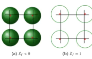
but presents two drawbacks. First, its accuracy is extremely low and can lead to a totally wrong approximation ofεfas illustrated
inFigure 3. Second,εftime variations are not smooth because
of the sudden consideration of a particle in a cell (out at tn−1 and in at tn). This jump leads to spurious oscillations, especially
due to the presence of the fluid volume fraction εf
time-derivative term in the degenerated Stokes problem (eq 5). The center particle method does not satisfy the basic time-step convergence property, and we have instead
ε − ε Δ = ±∞ Δ → − t lim t fn fn 0 1 (29)
Forfinite Δt, it also performs worse and worse as the fluid grid size decreases (since the particle volume isfinite, Δεf = εfn −
εfn−1increases as thefluid grid size decreases), hence impacting
the overall space convergence of the numerical method too. In order to improve thefluid volume fraction εfcalculation,
other methods were suggested in the literature as, e.g., the of fset
method of Alobaid et al.,19 the porous cube method of Link
et al.,36,37or more recently, the interesting mollif ication kernel/
Gaussian f iltering method of Pepiot and Desjardins.6 The
method we adopt in this work derives from the porous cube method proposed by Link et al. and assumes that the portion of the particle i belonging to a control volume k, i.e.,θi,k, can be approximated by the intersected volume of the smallest cube embedding the particle i (a cube whose edge length is equal to the particle diameter) and the control volume k.
θ = V V i k k i , approx cube, (30)
where Vcube,i = dp3 is the volume of the cube embedding the
spherical particle i and Vkapproxis the intersected volume of the
cube with thefluid cell k.Figure 4a shows the methodology in a 2D case, the extension to 3D is straightforward.
Our method smoothes out the calculation of the εf
time-derivative term in the degenerated Stokes problem (eqs 5) and recovers time convergence. This is a very important property. It also permits to use a smaller grid size than the particle center
method, i.e., down to ΔV ≃ 6Vp, while yielding a reasonably
accurate approximation ofεfas illustrated inFigure 4b. 2.6. Space/Time Complexity and Computing
Perform-ance. Bubbling and spouted fluidized beds are generally
considered as moderately dense to dense fluid/particles
sys-tems. In fact, the average porosityεfis≈ 0.7 in the bed (i.e., the
solid volume fraction is≈0.3 = 30%). Hence, the major part of
the computing time as well as the space/time complexity of our DEM-CFD model is related to particles. The time complexity
of particles motion is simply O(Ns), where Ns is the total
number of solid time steps performed over a simulation. The Lagrangian particle tracking and the computation of the hydrodynamic force ff p exerted on each particle scale linearly
with the total number of particles Np, i.e., O(Np). The com-putation of particles collisions theoretically scales as O(Np2),
but the use of a linked-cell spatial sorting reduces the space complexity to O(13NcNp), where Ncis the average number of
particles per linked cell. In fluidized bed simulations, Nc ≈ 1, such that the space complexity of particles collisions computa-tion is O(13Np). The overall space/time complexity of particles
motion is thus formally O(15NpNs) (we say “formally”, as
the constant 15 is not necessarily relevant). The projection
operator scales linearly with Np. The corresponding space
complexity is bounded by O(8Np) as a particle overlaps eight
fluid cells at most. The projection operator is used both for
Figure 3. Examples of particles/cell configurations illustrating the wrong evaluation of the fluid volume fraction by using the Particle Center Method.
Figure 4. Our embedding cube/square approximation method: (a) principle and (b) accuracy of the approximation as the evolution of particle volume crossing control volume l: (green dots) disc analytic solution, (blue line) our embedding square approximation method, (red dotted line) particle center method.
porosity and the three components of the velocity; hence, the
space complexity is bounded by O(32Np). As the projection
operator is used once perfluid time step, the overall space/time
complexity of our DEM-CFD model is O(15NpNs+32NpNf),
where Nfis the total number offluid time steps performed over
a simulation. Introducing the integer ratio of fluid time-step
magnitude over solid time-step magnitude rN = Δtf/Δtp, the space/time complexity of our DEM-CFD model can be for-mally rewritten as O((15 + 32/rN) NpNs). Dropping the
pre-factor 15 + 32/rN, the space/time complexity of our DEM-CFD
model is essentially O(NpNs).
The model presented previously has been implemented in
the fully MPI platform PeliGRIFF38 in order to simulate
systems containing up to a few tens of millions of particles. For fluidized beds and simple box geometries, a 2D domain
decomposition in the horizontal plane x−y (assuming gravity
and inlet velocity are in the vertical direction z) and a similar
domain decomposition forfluid domain and particles domain
supplies the best parallel performance. In fact, it guarantees a reasonably constant particle load balancing over time and sig-nificantly reduces the number of proc-to-proc (i.e., subdomain-to-subdomain) communications. Each subdomain slightly overlaps with its neighboring subdomains by (i) two layers of fluid grid cells to properly assemble all terms in the fluid conservation equations (and, in particular, the advection term with the second order TVD scheme) and (ii) a single layer of cells of the linked-cell grid to detect collisions with particles located in a neighboring subdomain.
Several simulations are performed on different configurations
in order to study the parallel scalability of our numerical imple-mentation. As we are interested in large-scale simulations, we evaluate the parallel scalability with weak scaling tests only. In other words, we set up the system in terms of a constant load per node, and we record the computing time as a function of the number of nodes with the size of the system increasing accordingly in the horizontal directions (which means that the height of the domain is constant while the cross section increases with the number of nodes). We present below results of a representative scalability test for a homogeneous bubbling fluidized bed. Features of the system are as follows:
• Inlet velocity at the bottom wall is constant in space and in time and is set to Uin= 3Umf.
• Boundary conditions on the lateral (vertical) boundaries are biperiodic.
• Each subdomain (i.e., core) has a size of 20dp× 20dp×
200dp.
• Grid size is set to Δx = 2.5dp, and hence, each subdomain
(i.e., core) contains 8× 8 × 80 = 5120 fluid cells. • Each subdomain (i.e., core) contains at the initial time
20× 20 × 200 = 80,000 spherical particles.
• Our jobs run on a 16-core per node supercomputer, so the reference for the weak scaling test is a full
node, i.e., a simulation on 16 cores with 16× 80,000 =
1,280,000 particles and 16× 5,120 = 81,920 fluid cells.
An ideal scalability means that the computing time is constant as the domain size and number of nodes increase
simul-taneously.Figure 5shows the evolution of the computing time
spent in each part of the code as a function of the number of nodes/system size. For the granular solver, we observe that after a rise of 5% between 1 and 2 nodes as a result of the internode communication overhead mainly related to the supercomputer architecture, the computing time keeps being
quasi-constant up to 32 nodes (i.e., 512 cores and 40,960,000 particles). This emphasizes the highly satisfactory parallel scal-ability of the granular solver. Concerning thefluid solver, the
advection−diffusion problem scales quite well up to 16 nodes/
256 cores and then a little less satisfactorily at 32 nodes/
512 cores. The decay of the scalability of the advection−
diffusion problem solution over 16 nodes/256 cores is not
entirely clear and is currently investigated in our group. It could be related to many diverse causes (as, e.g., the supercomputer network architecture on which jobs were run that groups 18 nodes together in a chassis; a 16 nodes job uses a single chassis of nodes, while a 32 nodes requires two chassis, and interchassis communication may cause an additional overhead) that are beyond the scope of this paper. The Stokes problem solution scales quite poorly as the number of nodes/cores increases. In fact, the computing time increases a lot from 1 node to 32 nodes. This was however predictable as the
number offluid cells per subdomain is rather low (due to the
fluid grid size constraint (eq 27), and the Stokes problem
involves the solution of a pressure Poisson problem solved in our code by an algebraic multigrid conjugate gradient method. It is known that the scalability of the multigrid method (or more generally any iterative solver) decays as the number of
nodes/cores increases if the number offluid cells (pressure
unknowns) per core is too small. This has been verified by
increasing the number offluid cells per core in the horizontal
direction from 8× 8 × 80 = 5120 to 32 × 32 × 80 = 81,920.
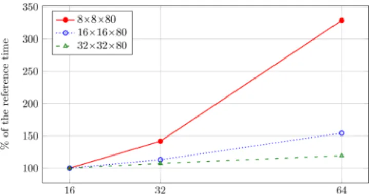
In fact,Figure 6clearly highlights that the multigrid solver for the pressure Poisson problem performs better and better in terms of parallel scalability as the load offluid cells per core
increases. Obviously, since a 32 × 32 × 80 subdomain now
hosts 16 times more particles, the total computing time increases accordingly although the parallel scalability
improves. However, even with a 8× 8 × 80 subdomain, the
overall parallel scalability is rather satisfactory. In fact, the red
line inFigure 5indicating the total computing time increase
for a given number of nodes with respect to a single node shows a linear trend with a very small slope. For 32 nodes/
512 cores/40,960,000 particles/2,621,440 fluid cells, this
increases is around 30% only, i.e., a parallel scalability of
100/130 ≃ 0.77. On the basis of this weak scaling test, we
believe that configurations similar to our representative test
(fluidized beds in a box geometry) in which dynamic load
balancing is not required can easily be simulated with our code with up to a few hundreds of millions of spherical particles on a few thousands of cores with a good parallel scalability, i.e., larger than 0.7, provided the load of particles per core is of the order of 105.
Figure 5. Scaling performance for a constant load per core (80,000 particles/5120 fluid cells). Evolution of the computational time spent in the various parts of the code as a function of the number of cores normalized by the time spent on a full node (16 cores).
3. SENSITIVITY OF THE MODEL TO NUMERICAL AND GEOMETRIC PARAMETERS IN THE CASE OF BUBBLING FLUIDIZED BEDS
As many variants of the two-way Euler−Lagrange model exist
as, e.g., formulations A and B,39contact solver,fluid flow solver, we would like to provide here a clear and detailed validation and sensitivity survey of our model that any other group can
reproduce. In this section, we consider bubblingfluidized beds
without wall effects. We first define statistical tools to analyze
the bed dynamics. Then, we examine the influence of the
following numerical parameters: solid time-step magnitude, fluid time-step magnitude, and fluid grid size on the computed
solution as well as the influence of the geometric size of the
domain in controlling the bubbling dynamics of the system.
3.1. Bed Statistics. A three-dimensional fluidized bed
generally comprises a large number of particles and exhibits a highly unsteady dynamics. As a result, the system can be characterized in terms of statictics only. It is hence crucial to define relevant statistical markers of the flow and a criterion to
assess the convergence of the statistics. We show in Figure 7
the typical time evolution of dynamic pressure drop across the bed together with the corresponding time evolution of bed
height for a homogeneous bubblingfluidization starting from
a bed at rest. All parameters of this simulation are listed in
Table 1. The early transient over which the bed expands a lot and the dynamic pressure drop across the bed overshoots is discarded in the analysis. Then, the bed transitions to its stationary (or pseudostationary) bubbling regime, and these two markers oscillate in time around their time-averaged value. In this stationary regime, we study particles trajectories sam-pled at a frequency fsample= 1/Δtsampleduring a time Tsample, and
we compute bed statistics. We define a criterion which permits
us to determine when statistics converge, i.e., when they remain
the same regardless of Tsample. For instance, let us consider the time-averaged sum of all particles velocity norm in the domain. It can be computed in the following way:
∫
∑
∑
∑
⟨ | |⟩ = | | ≈ | | + | | + = − = − = − + v v v v T t dt N t t Sum 1 ( ) 1 0.5( ( ) ( ) ) p X T t t T i N i T j N i N i j i j , sample 0 1 0 1 0 1 1 ss ss p T p sample sample sample sample (31)where Tsample = NTsampleΔtsample, tj = tss + jΔtsample, t0 = tss, and tNTsample= t0,s+ Tsample· tssdenotes the starting time of the pseu-dostationary regime or equivalently the end of the early
transient regime (Figure 7, tss = 1 s) . “X” means global
statistics, i.e., on all particles or in the whole domain. We
consider that the sample duration Tsample is large enough to
form relevant statistics once⟨Sum |vp|⟩X,Tsamplereaches a steady value. We therefore introduce the following convergence
criterion C:where and represent
the maximum and minimum values reached by⟨Sum|vp|⟩X,Tsample over [tss,tss+Tsample], and Tvar. is a time period of variation.
The maximum and minimum values of ⟨Sum|vp|⟩X,Tsample over
[tss,tss+Tsample] normalize C(Tsample,Tvar.). The convergence
criterion C(Tsample,Tvar.) contains one problem-dependent
time parameter Tvar.. To compute C(Tsample,Tvar.), we also
assume that Δtsample is a multiple of Δtf and that Tvar. is a multiple ofΔtsampleto avoid any interpolation in time.
Figure 6.Evolution of the scaling performace for the solution of the Stokes problem as a function of the number of cores for different fluid cells loads per core. The reference is the time spent on a full node (16 cores).
Figure 7.Time evolution of the bed height (dashed blue) and of the dynamic pressure drop across the bubbling bed (solid red).
Table 1. Parameters of Homogeneous Bubbling Fluidized Bed Considered To Illustrate Bed Statistics Convergence Criteriona
parameter value
particles
diameter dp 1 mm
densityρp 1500 kg m−3
dimensionless maximum overlapping distance δij,max/dp
0.05 stiffness coefficient kn 4000 N m−1
normal restitution coefficient en 0.9
Coulomb friction coefficient μC 0.4
solid time-step magnitudeΔtp 5× 10⁻⁶s
fluid
dimensionless mesh sizeΔx/dp 2
fluid time-step magnitude Δtf 2× 10⁻⁵s
densityρf 1.2 kg m−3 viscosityμ 1.8× 10⁻⁵Pa s fluidization velocity Umf(εf= 0.37) 0.315 m s−1 Uin/Umf 2.5 geometry domain size Lx× Ly× Lz 0.08 m× 0.08 m × 0.2 m
BC on lateral (vertical) boundaries biperiodic initial bed height H0 0.05 m (SCL)
number of particles 80× 80 × 50 = 320,000 dimensionless numbers
eUin
9 52.53
ρp/ρf 1500
aSCL means Simple Cubic Lattice to describe the initial layout of
For eachflow configuration, we set the values of Δtsampleand Tvar. using characteristic time scales as, e.g., time period of
pressure drop across the bed oscillations or average
convec-tive time scale of particles motion. Figure 8 shows the time
evolution of (Sum|vp|)X, ⟨Sum|vp|⟩X,Tsample and the convergence criterion described above. For that case, we assume that statistics are converged when C(Tsample,Tvar.) is less than 0.05
over Tvar.= 1 s. As shown inFigure 8, this condition is satisfied
for Tsample≃ 7.6 s.
3.2. Numerical Parameters. In order to perform simulations as accurate and reproducible as possible, we study
the influence of numerical parameters that have a major
influence on the computed solution. First, we study the
con-vergence of the numerical method with the solid andfluid
time-step magnitudes. Second, as an actual grid size convergence analysis cannot be conducted in relation to the grid size constraintΔV ≃ 10Vp, we identify what grid size offers the best
compromise between accurate resolution of the fluid flow
(small grid size) and relevant averaging process (large grid size).
The selected test case is once again a homogeneous bubbling fluidized bed. All simulation parameters are listed in Table 2. The configuration is similar to the one inSection 3.1, but the
flow regime is slightly more inertial ( eU = 301.33
in
9 versus
52.53 inSection 3.1).
3.2.1. Particle Time Step. In densefluidized bed simulations
performed with our DEM-CFD model, most of the computing
time is spent in the Lagrangian tracking of particles with collisions. In his pioneering work onDEM-CFD models, Tsuji7
emphasized that an accurate resolution of particle−particle
and particle−wall contacts is necessary to describe properly
the whole fluidized bed dynamics. As usual, we expect our
simulation method to be quick and accurate. These two expectations are generally contradictory as far as the time-step magnitude is concerned. In fact, a small time step guarantees accuracy but requires more time steps to be computed for the same physical time and vice versa for a large time step. As in a fluidized bed, the interphase coupling is dominant in the overall dynamics, determining the right compromise between accuracy and fast computing for the solid time-step magnitudeΔtpis not an easy task.
As presented in ref29, the collision characteristic time Tcol arising from the mass-spring-dashpot contact force model used in this work (seeSection 2.2) in the case of a normal gravityless collision of two spheres reads as follows:
π ω γ = − T n col 0 2 2 (33) with ω02 = 2k
n/mp. The normal dissipative coefficient γn can
be related to the coefficient of restitution en ∈ [0,1] in the
following way:γ = − ω π + n e e ln (ln ) n n 0 2 2. 29
As contacts are (very often explicitly) integrated in time in soft sphere models, this integration should be carried out at the discrete level with a
time stepΔtpmuch smaller than the contact duration Tcol to
guarantee an accurate resolution of the contact. Practically, it is recommended in the literature29,40,41to integrate a dry contact with Δtp in the range [Tcol/50, Tcol/15]. In a fluidized bed,
most contacts are physically different from an ideal normal
gravityless dry contact, and we hence rely on simulation tests to estimate the appropriate magnitude ofΔtp.
From Table 2 and eq 33, we have Tcol = 10−4 s. We fix Δx/dp= 2,Δtf= 2× 10⁻⁵s and perform a series of simulations
with a solid time stepΔtpin the range [0.25, 2]× 10−5s, i.e., Δtp∈ [Tcol/40, Tcol/5]. We compare statistics as a function of
Δtp in order to determine the maximal time-step magnitude
required in ourDEM-CFDsimulations to describe accurately the
bed dynamics. We plot inFigure 9the converged statistics of
the velocity norm of all particles⟨Sum|vp|⟩X,Tsampleas a function of the solid time stepΔtp. Here,⟨Sum |vp|⟩X,Tsampleconverges pro-gressively to a constant value asΔtpdecreases. ForΔtp≤ Tcol/10,
the dynamics of the bed seems to be unaffected by the
Figure 8.Time evolution of (Sum|vp|)X, its time average⟨Sum|vp|⟩X,Tsample
(above) and the convergence criterion C(Tsample,Tvar.) (below).
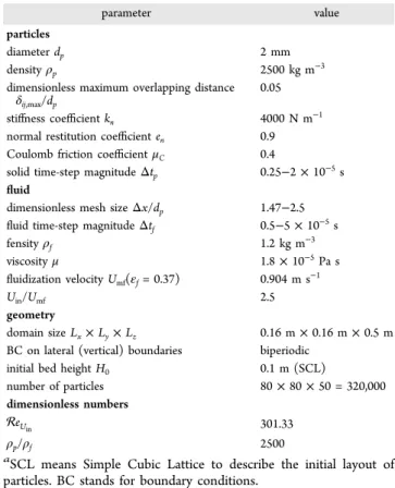
Table 2. Parameters of Homogeneous Bubbling Fluidized Bed Considered to Illustrate the Bed Statistics Convergence Criteriona
parameter value
particles
diameter dp 2 mm
densityρp 2500 kg m−3
dimensionless maximum overlapping distance δij,max/dp
0.05 stiffness coefficient kn 4000 N m−1
normal restitution coefficient en 0.9
Coulomb friction coefficient μC 0.4
solid time-step magnitudeΔtp 0.25−2 × 10⁻⁵s
fluid
dimensionless mesh sizeΔx/dp 1.47−2.5
fluid time-step magnitude Δtf 0.5−5 × 10⁻⁵s
fensityρf 1.2 kg m−3 viscosityμ 1.8× 10⁻⁵Pa s fluidization velocity Umf(εf= 0.37) 0.904 m s−1 Uin/Umf 2.5 geometry domain size Lx× Ly× Lz 0.16 m× 0.16 m × 0.5 m
BC on lateral (vertical) boundaries biperiodic initial bed height H0 0.1 m (SCL)
number of particles 80× 80 × 50 = 320,000 dimensionless numbers
eUin
9 301.33
ρp/ρf 2500
aSCL means Simple Cubic Lattice to describe the initial layout of
magnitude of Δtp. Interestingly, this upper bound for Δtp is
higher that the one generally used for dry granular simulations performed with the same DEM code that generally around Tcol/20.29 Actually, in a fluidized bed, particles motion is as
much driven by the hydrodynamic force ff pthan the collision
force fpp. For high Uin/Umf ratios, ff p actually dominates fpp. This sheds some light on why the dry granular upper bound is not directly applicable toDEM-CFDsimulations.
Another constraint on the solid time-step magnitude Δtp
common to dry granular simulations andDEM-CFDsimulations is
related to the maximum displacement of each individual par-ticle overΔtpwith respect to the maximum overlap distance per particle allowed over a contactδij,max(also referred to in DEM
models as crust thickness29). Indeed, in a soft sphere model, a particle should not move more than its crust thickness overΔtp,
otherwise two colliding particles may overlap more than allowed to. This condition reads as follows:
δ = vΔt < CFL ij p 1 ij particle ,max (34)
where vijis the relative velocity between colliding particles i and
j. It is somehow similar to a Courant−Friedrichs−Lewy (CFL)
stability condition for the fluid motion. The crust thickness
δij,maxis afixed simulation parameter, set in our simulations to
δij,max/dp= 0.05 (Table 2). An upper bound for vijneeds to be
estimated before the simulation in order to properly set Δtp
according to relation 34. Note that our DEM solver uses a
constant time-step integration and is not able to perform local time-step adaption. In practice, as the estimation of the upper
bound for vij is not straightforward, we introduce a safety
coefficient of 2 and require the following condition CFLparticle<
0.5 to be satisfied.
In the case of homogeneous bubbling fluidized beds with
an inlet velocity Uin ranging from Umf to 7Umf, extensive
computing indicates that the following empirical formula:
| | =̂ ⎛ ⎝ ⎜ ⎞ ⎠ ⎟ U U U vp 2 inln in mf (35)
is a reliable approximation of the maximum particle velocity norm (in the sense over all particles and a long enough
sim-ulation time). Thus, the solid time stepΔtp in homogeneous
bubblingfluidized bed simulations is set as a combination of
theCFLparticlecondition and the contact integration condition as
follows: δ Δ = | | ̂ ⎛ ⎝ ⎜⎜ ⎞ ⎠ ⎟⎟ t T v min 10 , 0.5 p ij p col ,max (36)
3.2.2. Fluid Time Step. The explicit treatment of the
advective term in thefluid momentumeq 4requires the fluid
time stepΔtfto satisfy aCFLcondition to ensure stability. For
constant grid sizeΔx in all 3 directions, theCFLcondition reads
as follows: = | |Δ Δ < = u t x CFL max max CFL d j f d j f 1,2,3 , , max (37)
where d denotes the space direction index, j the velocity node index, and uf,d,jthe d component of ufat velocity node j. For our
first-order explicit treatment of the advection term, CFLmax is
theoretically 1. In practice, we use a safety coefficient of 2 and imposeCFL < 0.5 instead. As for the granular time-step
mag-nitude Δtp, we do not known a priori what will be the value
of maxd=1,2,3 maxj |uf,d,j| over a whole simulation. Extensive
computing indicates that high solid volume fraction hetero-geneities lead to local velocity overshoots as large as 10 times
the inlet velocity. Then, a first constraint to determine the
magnitude ofΔtfis as follows: Δt < Δx U 0.5 10 f in (38)
However, contrary to the granularflow solver, the fluid solver
possesses a local time adaption mechanism to ensure stability by temporarily splitting the diffusion−advection problem (eq4)
into a separate diffusion subproblem and a separate advection
subproblem and subtime stepping the advection subproblem
such that eq 37 is recovered. The advection subproblem is
hence solved m consecutive times with a time step Δtadv as
follows: ρ ̃ − ̃ ρ Δ = − ∇· ̃ ̃ = − + + − + − + + u u t u u k m ( ), 0, ..., 1 f f n f n k m f n f n k m f f n f n k m fn k m ( 1)/ 1 / adv 1 / / , , , (39)
withΔtadvsatisfying (37), m× Δtadv= Δtf, ũfn= ufnand uf* =
ũfn+1. It is recommended not to perform these subiterations too
often over a simulation as it affects the time accuracy of the
solution. If this does happen too often, it is safer to redo the simulation with a smallerΔtf.
The second constraint to determine Δtf derives from the
loose (explicit) coupling of the fluid and solid governing
equations in our solution algorithm. In fact, we solve thefluid
governing equations for a fixed position and reaction source
term of the particles computed at the previous time and then
advance the particles for afixed hydrodynamic force exerted on
them. In other words, the particles as seen by the fluid are
frozen overΔtfand similarly thefluid as seen by the particles is
frozen over Δtf. IfΔtf is “small enough”, this loose coupling strategy yields a reasonably accurate time evolution of the system. However, to the best of our knowledge, there is no theoretical way to estimate an upper bound ofΔtfthat enables
one to avoid a nonphysical and nonrealistic evolution of the system. Hence, we rely once again on extensive computing to
empirically determine the optimal magnitude of Δtf. We fix
Δx/dp= 2,Δtp= Tcol/20 = 5× 10⁻⁶s and perform a series of
simulations with a fluid time step Δtf in the range [Tcol/20, Tcol/2]. In all these simulations,Δtfsatisfies eq37. We compute
Figure 9.Influence of solid step magnitude (red line), fluid time-step magnitude (red dotted line), andfluid grid size (blue dotted line) on the time-averaged sum of all particles velocity norm, selected as a major feature of the computed solution.
the statistics of the bed as a function ofΔtf. InFigure 9, we plot as a dashed red line the velocity norm of all particles ⟨Sum|vp|⟩X,Tsample versus Δtf. For Δtf < Tcol/5,⟨Sum|vp|⟩X,Tsample is almost independent ofΔtf, giving an upper bound for describing
properly the bed dynamics. Since the solution of the fluid
problem is rather computationally inexpensive with respect to the Lagrangian tracking of particles with collisions, a sensible guideline seems to beΔtf≤ Tcol/5. This guideline has proven to
be reliable in our simulations. Note that the loose coupling of
the fluid and solid governing equations can be improved in
different ways as, e.g., (i) using a second order time accurate
leapfrog algorithm for the fluid solver in the same spirit as
the granular solver or (ii) interpolating thefluid velocity field at particles positions both in time and in space as particles
move and hence update fpp at each granular solver subtime.
Improvement (ii) will increase considerably the computing cost but should enable us to compute solutions of higher precision and stability. This is a topic of ongoing work for the
enhance-ment of ourDEM-CFDmodel.
3.2.3. Fluid Grid Size. OurDEM-CFDnumerical model is based
on a unique grid to solve the Navier−Stokes equations, to
compute, and to compute thef fluid−solid interphase
coupl-ing. In other words, contrary to, e.g., ref 6, our projection
operator from Lagrangian to Eulerian depends on the grid size Δx. A true grid size convergence analysis cannot be performed asΔx must satisfy (30) or at least Vp< Δx3to avoid ,f = 0
(Section 2.5). In any case, Δx cannot tend to zero as in a classical grid size convergence analysis. What we can however investigate in the rangeΔx ∈ [1.47 dp; +∞] is the lower and
upper bounds of Δx to guarantee quasi-grid independent
computed results. Once again, the method requires a large
enoughΔx for the spatial averaging process and a small enough
Δx to properly capture the fluid flow dynamics. To estimate the optimal grid size range, wefix Δtp= Tcol/20 = 5× 10⁻⁶s,Δtf=
10−5s = 2Δtpand perform a series of simulations with Δx ∈
[1.47 dp, 3.57 dp]. We plot⟨Sum|vp|⟩X,TsampleversusΔx inFigure 9 as a representative measure of bed statistics. It is pretty visible that bed statistics are quasi independent ofΔx for Δx ∈ [1.85 dp, 2.5 dp]. The trend is similar for other measures of bed statistics. The lower bound is in agreement with the
theoretical lower bound (eq 27) for the separation of scales
(1 order of magnitude) as originally introduced by.42 All
simulations in the rest of the paper are performed withΔx close to 2 dp.
3.3. Domain Size Influence. In fluidized beds, large flow
structures such as particles clustering, i.e., regions of low , ,f
andfluid bubbles, i.e., regions of high, (close to 1), developf in the core of the bed. The size of these structures is controlled
by theflow regime, i.e., the dimensionless numbers that govern
the system (density ratio, Reynolds number, Uin/Umfratio), and the lateral boundary conditions. Although it is known (and rather intuitive) that the domain size controls the dynamics of the system with lateral solid wall boundary conditions (no slip
condition on the fluid velocity), biperiodic domains are
assumed to represent infinitely large domains in directions of
periodicity. However, the size of the computational domain in each periodic direction needs to be larger than the characteristic length scale of the system dynamics for this assumption to hold.
If this assumption is not satisfied, the size of these
repre-sentative flow structures (essentially fluid bubbles) can match
the domain size, and then, a bubbling bed can degenerate into a
slugging bed as presented in Figure 10, even with biperiodic
boundary conditions. In fact, if the domain is transversely (horizontally) too narrow and a particles cluster is as large as
the domain cross section, thefluid cannot easily flow through
this cluster. Instead, afluid bubble manifests upstream of the
particles cluster, grows, and carries upward the cluster as an
homogeneous dense pack of particles, as shown inFigure 10b.
Particles progressively plummet downward from the bottom of the cluster to the bottom of the bed until the cluster vanishes and another cluster (slug) appears. This cyclic slugging
behavior is representative of narrow fluidized beds. In fact,
the primary instability, i.e., the vertical instability, can develop while the secondary transverse instability is damped by the narrowness of the domain. Conversely, with all other param-eters kept the same, if the domain cross section is large enough, in the sense larger than the largest particles cluster, the fluid flows across these clusters more easily, and the secondary transverse instability develops. As shown inFigure 10a, the size of created bubbles is not controlled by the domain cross section, and the bed dynamics is totally different.
From these preliminary results, it is rather remarkable that
the bed dynamics is strongly affected by the computational
domain periodic size. A valuable question to answer is the
minimum domain size for a certainflow regime to exhibit
cross-section size-independent bed statictics and behavior, such that the biperiodic simulation indeed represent an infinitely larger fluidized bed. Performing computations in a small biperiodic domain is tempting as it involves less computing resources but at the cost of producing physical results biased by the domain cross-section size.
To highlight the influence of the cross-section size of
biperiodic domains, we perform a series of simulations in domains of increasing cross-section size and examine how this affects bed statistics, in the same manner as in ref6. This sur-vey is carried out with three-dimensional systems as two- and three-dimensional beds do not lead to the same statistics and
presumably to different dynamics. The initial configuration is
a simple cubic arrangement of 50 particles height, and the number of particles and the domain size in the transverse direc-tions are increased simultaneously. Simuladirec-tions are performed on domains with a cross section in the range of 20dp× 20dpto
120dp × 120dp. All other parameters are similar to the ones
used in Section 3.1and listed inTable 1. Converged in time
bed statistics are plotted inFigure 11. The top row shows axial profiles of time-averaged porosity ⟨ ⟩,f Tsample and time-averaged particles velocity norm⟨Sum|vp|⟩Tsampleand the bottom row their corresponding time variance. Please note that⟨Sum|vp|⟩Tsampleis
Figure 10.Snapshots at t = 2.8 s of thefluid volume fraction spatial distribution in a homogeneous bubblingfluidized bed in a vertical cut plane for domains with (a) a wide cross section and (b) a narrow cross section.