Perceiving perpendicular and parallel contours in the frontoparallel plane
Ekaterina Koshmanova, Tadamasa Sawada
School of Psychology, National Research University Higher School of Economics.
Abstract
The perception of a pair of contours in a retinal image cannot be understood simply by adding up the perceptions of the individual contours, especially when they form a perpendicular junction, or are parallel to one another. It is the relationship among the contours that determines what is perceived. Note that it is hard to actually compare the perception of such configurations quantitatively. We managed to do this by testing the perception of such configurations in three psychophysical
experiments in which the perception was characterized by measuring the orientation threshold of a single contour. This threshold was estimated by using a modified Method of Constant Stimuli based on the assumption that contours forming a configuration are perceived individually, and that they are integrated linearly. This assumption made the quantitative comparison of the perceived
configurations possible. We found that changes of the estimated threshold depended on the type of the configuration, specifically thresholds estimated from a perpendicular junction were substantially lower than thresholds estimated from a single contour or from a non-perpendicular junction. The lowest thresholds were observed when the threshold was estimated from a pair of parallel contours. These results suggest that the visual system is sensitive to perpendicular junctions and parallel contours in a retinal image.
Keywords: orientation discrimination; angle discrimination; orientation threshold; parallelism; perpendicularity; Method of Constant Stimuli; contour configuration
1
Abstract
The perception of a pair of contours in a retinal image cannot be understood simply by adding up the perceptions of the individual contours, especially when they form a perpendicular junction, or are parallel to one another. It is the relationship among the contours that determines what is perceived. Note that it is hard to actually compare the perception of such configurations quantitatively. We managed to do this by testing the perception of such configurations in three psychophysical experiments in which the perception was characterized by measuring the orientation threshold of a single contour. This threshold was estimated by using a modified Method of Constant Stimuli based on the assumption that contours forming a configuration are perceived individually, and that they are integrated linearly. This assumption made the quantitative comparison of the perceived configurations possible. We found that changes of the estimated threshold depended on the type of the configuration, specifically thresholds estimated from a perpendicular junction were substantially lower than thresholds estimated from a single contour or from a non-perpendicular junction. The lowest thresholds were observed when the threshold was estimated from a pair of parallel contours. These results suggest that the visual system is sensitive to perpendicular junctions and parallel contours in a retinal image.
Keywords: orientation discrimination; angle discrimination; orientation threshold; parallelism; perpendicularity; Method of Constant Stimuli; contour configuration
Introduction
Contours are important elements of a retinal image because they play a critical role in visual perception of a shape (Biederman, 1987; Pizlo, 2008). Contours have orientation information at every straight or smoothly curved point along them. It is this property that distinguishes them from discrete dots. In this study, we only consider a straight contour (a line segment) for purposes of simplicity. The perception of the orientation of contours has been extensively studied systematically in psychophysics. All of these studies used a discrimination threshold that was usually measured with the Method of Constant Stimuli. The threshold characterizes width (e.g. standard deviation) of a normal distribution whose cumulative function is fitted to psychophysical data. These thresholds represent the uncertainty of the perception of the orientation of the contour. The studies showed that the contour orientation threshold becomes lower as the contour becomes longer (Mäkelä, Whitaker, & Rovamo, 1993; Vandenbussche, Vogels, & Orban, 1986; Watt, 1987), becomes thinner (Mäkelä,
2 Whitaker, & Rovamo, 1993), and is presented closer to a fixation point (Mäkelä, Whitaker, & Rovamo, 1993; Vandenbussche, Vogels, & Orban, 1986; Watt, 1987). The threshold also becomes lower when the orientation of the contour is closer to the vertical or horizontal than it is with any of the other orientations ( Andrews, 1967; Chen & Levi, 1996; Heeley & Buchanan-Smith, 1990, 1996; Westheimer, 2001; Sysoeva, Davletshina, Orekhova, Galuta, & Stroganova, 2016).
The orientation threshold can also be affected by the experimental procedure. The threshold is lower when the two contours are presented simultaneously than it is when the contours are presented sequentially (Chen & Levi, 1996; Regan, Gray, & Hamstra, 1996; Heeley & Buchanan-Smith, 1996). In these studies, the threshold for the simultaneous presentation was estimated from performance of a participant in judging whether the relative orientation of the contours is smaller or larger than a standard angle. The participant was not explicitly given the standard angle but
estimated it from some trials. The threshold for the simultaneous presentation depends on the relative orientation of the contours (Chen & Levi, 1996; Heeley & Buchanan-Smith, 1996, see also Regan et al., 1996). The lowest threshold is observed when the standard angle is 90° and the contours are perpendicular to one another. The threshold also becomes this low when the standard angle is 180° and the contours become collinear to one another.1 Note that orientations of the perpendicular and collinear configurations of contours were not fully randomized in experiments of these studies in which perception of both of these configurations were tested. Then, the measured thresholds with these configurations could be also affected by orientations of individual contours forming the configurations. It is because a discrimination threshold of an orientation of a single contour is lower when its orientation is around vertical or horizontal than any of the other orientations (Westheimer, 2001).
A pair of contours is more regular when they form a perpendicular junction or when they are parallel2 to one another (Metzger, 1936/2006; Koffka, 1935). These configurations are processed faster by the visual system than less regular configurations are (Feldman, 2007; Kubilius, Sleurs, & Wagemans, 2017). It seems possible that a parallel configuration will affect the orientation threshold of a contour as much as the perpendicular configuration does. Note, however, that it is difficult to
1The orientation threshold under this collinearity condition is essentially the same as a chevron threshold but it has a different
parameterization (Andrews, Butcher, & Buckley, 1973; Tyler, 1973; Watt, 1984).
2 Contours that are collinear to one another can be regarded as being also parallel to one another. On the other hand,
parallel contours are not necessarily collinear. In this study, we use “parallel” to mean contours that are parallel but are not collinear to one another. These two types of contour configurations can play different roles for visual perception (Biederman, 1987; Leeuwenberg & van der Helm, 2013; see also General Discussion).
3 compute orientation thresholds that reflect the effects of different configurations in such a way that they can be compared with one another.
In this study, we studied the perception of the configurations of contours by using the orientation threshold of a single contour. This orientation threshold represents uncertainty of perceived orientation of the single contour and was estimated by using a modified Method of Constant Stimuli that can take the contour configurations into consideration. The modified Method of Constant Stimuli was based on the assumption that the contours making up a particular
configuration are perceived individually from one another, and that the composition is perceived as a linear combination of the individual contours perceived (see Appendix for details). The orientation threshold was estimated using different psychophysical functions for the individual configurations. These psychophysical functions were derived based on this assumption and were controlled by the orientation threshold. If the assumption of the modified Method of Constant Stimuli is correct, this threshold should remain constant with all of the configurations. In other words, the difference of the thresholds measured with different configurations represents differences in processing in the visual system while it suggests that the assumption is violated. The orientation threshold measured using the modified Method of Constant Stimuli is used as a descriptive value of this visual process in this study. A lower threshold for a particular configuration suggests that this configuration was
processed more precisely and accurately than the others. So, the modified Method of Constant Stimuli allows us to compare the perceived configurations quantitatively.
General Method
ApparatusThe experiments were conducted in a completely dark room. The stimuli were displayed on a 120Hz 24-inch LCD monitor (BenQ Zowie XL2411) controlled by a computer. The resolution of the monitor’s screen was 1920 × 1080 pixels, and its size was 53.1 × 29.8 cm. The viewing distance was 160 cm, and Observer’s head was supported by a chinrest. The screen was vertical and
frontoparallel to the Observer’s head. Viewing was binocular, and the center of the screen was positioned at Observer’s eye-level. A black panel (57 × 50 cm) with a circular aperture (29 cm in diameter) was attached to the monitor to avoid the parallel and perpendicular edges between the screen and the monitor's frame to serve as an artifactual reference for judging the orientations of contours in the experiments.
4
Stimuli
All of the stimuli were composed of one or two contours. The length of the contour was 16.0 ± 2.0 cm (5.71 ± 0.71 deg) in Experiments 1 and 2. Their width was 1.0 mm (2.15 arcmin). The eccentricity of the contour depended on the experimental conditions, but it was never more than 3.3 cm (1.18 deg). The contours were long enough to guarantee that an orientation threshold would not be affected by the eccentricity of the contour within this range (Andrews, 1967; Mäkelä, Whitaker, & Rovamo, 1993; Vandenbussche, Vogels, & Orban, 1986; Watt, 1987). The contours, drawn in white (297 cd/m2), were seenon a dark background (0.48 cd/m2).
Procedure
The experiments reported in this study were conducted in accordance with the Code of Ethics of the World Medical Association (Declaration of Helsinki).
The Method of Constant Stimuli with a two-alternative-forced-choice design was used in all of the experiments. The Observers' tasks depended on the specific conditions (see the Method sections for the conditions). The experimental sessions were controlled by a program developed with Visual C++.
Each trial began by fixating a small point for 250 ms, after which a mouse button was pressed which caused two intervals of visual stimuli to be shown. The duration of each visual
stimulus was 250 ms with a 250 ms inter-stimulus interval. A response screen appeared 250 ms after the disappearance of the 2nd stimulus. The response screen displayed two choices and the Observer chose one by using the mouse. The Observers were informed about the accuracy of their response when they responded. The trials were self-paced.
All of the experimental conditions were blocked within each session. The Observer
participated in two sessions for each condition of the experiment. The Observer ran his first session, which contained all of the conditions in a random order. He ran his second session in the reverse of this order. The Observer was informed the condition coming up before each session. Each session consisted of 160 trials with their order randomized. An orientation threshold, which represented the uncertainty of the Observer's orientation perception of a single contour, was estimated for each session.
The Observers were the authors of this study (EK and TS). Eleven volunteers, with normal or corrected-to-normal vision, also participated. They had no prior experience in psychophysical
5 experiments. Informed consents were obtained from all of them. The authors participated in all the experiments. Each of the volunteers participated in one of the experiments, except for AP. AP only participated in Experiment 1 and its control experiment.
Experiment 1
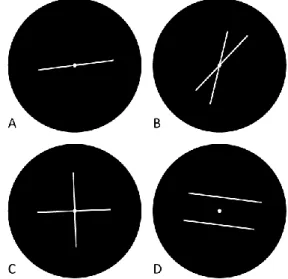
In Experiment 1, we measured the orientation threshold for the 4 types of contour configurations shown in Figure 1, specifically: (i) a single contour (Condition-A), (ii) a 30° X-junction (Condition-B), (iii) a perpendicular X-X-junction (Condition-C), and (iv) a pair of parallel contours (Condition-D).
Figure 1. The 4 types of contour configurations used in Experiment 1: (A) a single contour, (B) a 30° X-junction, (C) a perpendicular X-junction, and (D) a pair of parallel contours. Black circles represent the circular aperture (29 cm in diameter) of the apparatus. The contours, which were 1.0 mm (2.15 arcmin) wide in the visual stimuli, are wider in this figure to make them visible.
Method
In Condition-A, the orientation threshold was estimated from only a single contour. In each trial, two, 250 ms presentation intervals of single contours, were shown at the center of the screen. The orientation of the first contour was random, and the orientation of the second contour was made relative to the first contour as follows: by -6.40°, -4.50°, -2.70°, - 0.90°, 0.90°, 2.70° , 4.50°, or 6.40°. The Observer judged whether the second contour shown was rotated clockwise or
6 relative orientation in a single session. The frequency of counterclockwise responses was plotted for each session as a function of its relative orientation. This plot was fitted with a cumulative normal distribution function. The standard deviation of this function represents the discrimination threshold of the orientation between the two contours. The orientation threshold of a single contour was computed by dividing the standard deviation by 20.5 (Chen & Levi, 1996, see Appendix).
In Condition-B, the orientation threshold was estimated from an X-junction of 30°. In each trial, two, 250 ms presentation intervals of X-junctions, were shown at the center of the screen. The orientation of each junction was random. In the first interval, the narrower angle of the junction was 30° ± 0.90°, 2.70°, 4.50°, or 6.40°. It was always 30° in the second interval. The Observer indicated which interval had the most acute angle.3 The Observer ran 20 trials for each of the eight different junction angles in a single session. The frequency of the responses in which the second junction was more acute was plotted in each session as a function of the junction’s angle in the first interval. This plot was fitted with a cumulative normal distribution function, and the orientation threshold of a single contour was computed by dividing the standard deviation of the fitted function by 2 (see Appendix).
In Condition-C, the orientation threshold was estimated from a perpendicular X-junction. In each trial, two, 250 ms presentation intervals of perpendicular and nearly-perpendicular X-junctions were shown at the center of the screen. The orientation of each junction was random. The angle of the nearly-perpendicular junction was 90° + 0.60°, 1.20°, 1.80°, 2.40°, 3.00°, 3.60°, 4.20°, or 4.80°. The Observer ran 20 trials for each of the eight nearly-perpendicular angles. The perpendicular junction was shown in the first interval for 10 of the 20 trials, and in the second interval for the other 10 trials. The Observer indicated which interval had the perpendicular junction. The frequency of correct responses was plotted respectively for two sets of trials in which the perpendicular junction was shown in the first and second intervals. These two plots are functions of the
nearly-perpendicular angles. They were analyzed by using a modified Method of Constant Stimuli (see Appendix). This modified Method of Constant Stimuli characterizes the two plots with the orientation threshold of a single contour, and the response bias between the two intervals.
3We could have randomized the order of the intervals and asked the Observer to indicate which interval had the X-junction of 30° in
Condition-B . Had this been done, the hypothetical task in Condition-B would have been more similar to the tasks in Conditions-C and -D. Note that the task required the Observer to memorize a 30° angle in a single session of Condition-B, and that this could be difficult. A perpendicular junction (Condition-C), and a pair of parallel contours (Condition-D) are considered to be regular (see Metzger, 1936/2006; Koffka, 1935) but a junction of 30° is not considered to be regular.
7 In Condition-D, the orientation threshold was estimated from a pair of parallel contours. In each trial, two, 250 ms presentation intervals of parallel and nearly-parallel contours were shown. The eccentricity of each contour was random between 3.0 ± 0.3 cm (1.07 ± 0.1 degrees). The orientation of each pair of contours was random. The relative orientation between the pair of nearly-parallel contours was 0.60°, 1.20°, 1.80°, 2.40°, 3.00°, 3.60°, 4.20°, or 4.80°. The Observer ran 20 trials for each of the eight nearly-parallel orientations. The pair of parallel contours was shown in the first interval for 10 of the 20 trials, and in the second interval for the other 10 trials. The
Observer indicated which interval had the parallel contours. The frequency of correct responses was plotted respectively for two sets of trials in which the parallel contours were shown in the first and second intervals. These two plots are functions of the nearly-parallel orientations. They were
analyzed by using a modified Method of Constant Stimuli (see Appendix). This modified Method of Constant Stimuli characterizes the two plots with the orientation threshold of a single contour, and the response bias between the two intervals.
Results
Figure 2 shows the estimated orientation thresholds observed in Experiment 1 for individual Observers. It also shows their averaged results. The ordinate shows the estimated orientation
threshold. The symbols show the 4 types of the configurations. These results were analyzed by using a one-way ANOVA within-subjects design. The Main effect of the type of configuration was
significant (F3,15 = 44.58, p = 1.04 × 10⁻⁷). Recall that these orientation thresholds were estimated under the assumption that the contours that made up a specific configuration were perceived
individually, and that the complete visual composition was perceived as a linear combination of the individual contours perceived. If this assumption is correct, the threshold would be constant across the types of configurations. The effect of the type of configuration observed suggests that this assumption is not valid.
8 Figure 2. shows the results obtained in Experiment 1. The ordinate shows the orientation threshold, and the symbols shows the 4 types of the configurations. (A) Results of individual Observers. Error bars show the standard errors calculated from two sessions for each condition. (B) Averaged results from all six Observers. Error bars show the standard errors calculated from 6 Observers.
The results described above can be interpreted as showing that the visual system is more sensitive to contour configurations that have lower thresholds. An a posteriori test showed that the orientation threshold was high in the following order of Conditions-A, -B, -C, and -D (A vs. B, t(5) = 3.86, p = 0.0355; B vs. C, t(5) = 6.47, p = 0.00394; C vs. D, t(5) = 3.95, p = 0.0324, where the p-values were multiplied by 3 as a Bonferroni adjustment). These results suggest that the visual system is sensitive to perpendicular junctions, and is even more sensitive to parallel contours. Note that in Condition-A, the Observer had to use a common world coordinate system between the two intervals in each trial to be able to compare the orientations of the two contours. Also note that this
9 was not the case in the other conditions. Here, the Observer compared the relative orientation
between a pair of contours in the first interval with the relative orientation between another pair of contours in the second interval of Conditions-B, -C, and -D. This task did not require using the common world coordinate system between the intervals. The highest threshold, which was observed in Condition-A, can be explained by the fact that a common coordinate system between the two intervals was required.
Control Experiment
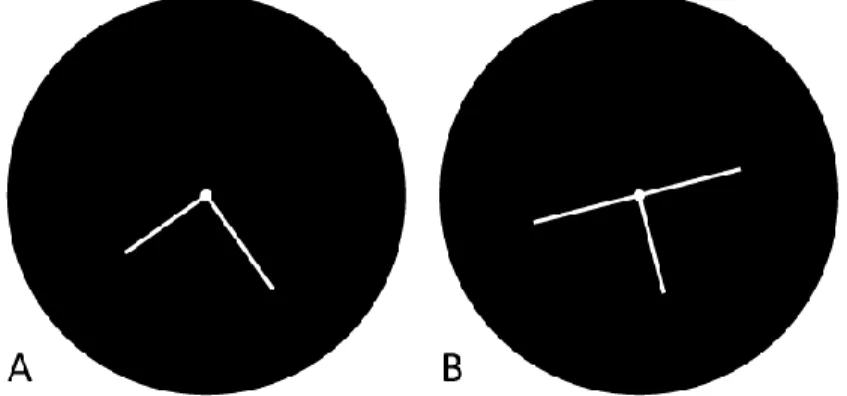
We tested only an X-junction (Condition-C) when we measured the orientation threshold with a perpendicular junction in Experiment 1. Note that there have been suggestions that the human visual system is more sensitive to L- and T-junctions than to the X-junction (Kubilius, Sleurs, & Wagemans, 2017). In a control experiment, run to confirm this, the orientation threshold was measured for 3 types of perpendicular junctions: (i) an L-junction, (ii) a T-junction, and (iii) an X-junction. The condition of the X-junction in the control experiment was identical with Condition-C in Experiment 1. The conditions of the L- and T-junctions in the control experiment, were the same as Condition-C with the following exception: The T- and L-junctions were generated by deleting parts of the contours that composed the X-junction. This operation made one (T-junction) or both (L-junctions) contours shorter (8.0 ± 1.0 cm, 2.86 ± 0.36 deg). They were still long enough to allow us to believe that their length would not affect the orientation threshold (Watt, 1987). The junctions were shown at the center of the screen in all the conditions.
Figure 3. Two of the 3 types of junctions used in the control experiment: (A) an L-junction and (B) a T-junction. Black circles represent the circular aperture (29 cm in diameter) of the apparatus. The contours, which were 1.0 mm (2.15 arcmin) wide in the visual stimuli, are wider in this figure to make them visible.
10 Figure 4 shows the estimated orientation thresholds observed in Experiment 1 for individual Observers. It also shows their averaged results. The ordinate shows the estimated orientation
threshold. The symbols show the 3 types of the junctions. These results were analyzed by using a one-way ANOVA within-subjects design. The Main effect of the type of junction was significant (F2, 10 = 4.235, p = 0.047). But note that an a posteriori test did not show any significant pair-wise difference (X vs. L, t(5) = 3.31, p = 0.0640; X vs. T, t(5) = 0.935, p = 1.0; L vs. T, t(5) = 1.77, p = 0.412, where the p-values were multiplied by 3 as a Bonferroni adjustment). These results suggest that the type of junction is not critical for the human's sensitivity to a perpendicular junction.
Figure 4. shows the results obtained in our control experiment for 3 types of junctions. The ordinate shows the orientation threshold, and the symbols show the 3 types of junctions. (A) Results of individual subjects. Error bars show the standard errors calculated from two sessions for each condition. (B) Averaged results from all three subjects. Error bars show the standard errors calculated from 6 Observers.
11
Experiment 2
Results of Experiment 1 show that the Observer is more sensitive to a pair of parallel
contours (Condition-D) than to a perpendicular junction (Condition-C). The contours that composed the perpendicular junction always intersected with one another at the center of the screen. This means that their eccentricity was always 0 from the center in Condition-C. But, the eccentricity of the parallel contours was different, namely, it was located randomly between 3.0 ± 0.3 cm (1.07 ± 0.1 degrees) from the center. The difference in the orientation thresholds observed between these two conditions might have been underestimated because of this difference in eccentricity. In
Experiment 2, we controlled the eccentricity of the contours systematically so we were able to make a more direct comparison of the orientation thresholds with perpendicular junctions and the parallel contours.
Method
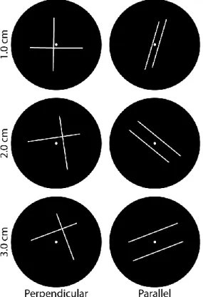
Figure 5 shows the six (2 X 3) experimental conditions namely, the 2 types of contour configurations (a perpendicular X-junction or a pair of parallel contours) and the 3 levels of eccentricity of the individual contours from the center of the screen (1.0 cm, 2.0 cm, or 3.0 cm). Random noise (± 0.3 cm) was added to the eccentricity. The X-junction was not shown at the center of the screen in any of the eccentricity conditions. The parallel contours condition with an
eccentricity of 3.0 cm (± 0.3 cm) was the same as Condition-D in Experiment 1.
In each trial, two, 250 ms presentation intervals of configurations of contours were shown. The orientation of each configuration was random. One of the configurations was regular, namely, a perpendicular junction in a session with the perpendicular junction condition, and a pair of parallel contours in a session with the parallel contours condition. The other configuration was nearly-regular. The relative orientation between the contours of the nearly-perpendicular junction was 90° + 0.60°, 1.20°, 1.80°, 2.40°, 3.00°, 3.60°, 4.20°, or 4.80°. The relative orientation between the pair of nearly-parallel contours was 0.60°, 1.20°, 1.80°, 2.40°, 3.00°, 3.60°, 4.20°, or 4.80°. The Observer ran 20 trials for each of the eight nearly-regular configurations. Regular configurations were shown in the first interval for 10 of the 20 trials, and in the second interval, for the other 10 trials. The Observer indicated which interval contained the regular configuration. The Observers' responses were analyzed by using a modified Method of Constant Stimuli (see Appendix).
12 Figure 5. The 2 types of configurations of contours with the 3 levels of eccentricity of the individual contours from the center of the screen used in Experiment 2. Black circles represent a circular aperture (29 cm in diameter) in the apparatus. The contours, which were actually 1.0 mm (2.15 arcmin) wide in the visual stimuli, were made wider in this figure to make them visible.
Results
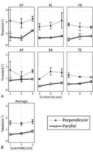
Figure 6 shows the estimated orientation thresholds observed in Experiment 2 for individual Observers. It also shows their averaged results. The ordinate shows the estimated orientation
threshold. The abscissa shows the 3 levels of eccentricity. The symbols show the 2 types of configurations. These results were analyzed by using a two-way ANOVA within-subjects design: the 2 types of configurations of contours (a perpendicular X-junction or a pair of parallel contours) and the 3 levels of eccentricity of the individual contours from the center of the screen (1.0 cm, 2.0 cm, or 3.0 cm). The Main effect of the type of configuration was significant (F1, 25 = 138, p = 1.13 × 10⁻¹¹). The Main effect of the eccentricity (F2, 25 = 2.90, p = 0.073), and the interactions between the
13 type of configuration and the eccentricity (F2, 25 = 0.466, p = 0.633), were not significant. These results also show that the visual system is more sensitive to parallel contours than to perpendicular junctions. The sensitivity to these configurations is robust against the eccentricity of the contours that composed the configurations within the range tested in Experiment 2.
Figure 6. shows the results obtained in Experiment 2. The ordinate shows the orientation threshold, the abscissa shows the 3 levels of the eccentricity, and the symbols shows the 2 types of the
configurations. (A) Results of individual Observers. Error bars show the standard errors calculated from two sessions for each condition. (B) Averaged results from all six Observers. Error bars show the standard errors calculated from 6 Observers.
14
Summary
Our experiments showed that the visual system is sensitive to perpendicular junctions, and it is even more sensitive to pairs of parallel contours. The orientation threshold of parallel contours was lower than the threshold of perpendicular junctions by a factor of 0.71 in Experiment 1, and, on average, by a factor of 0.44 in Experiment 2.
It is worth noting that the Observers were biased to respond that the configuration of the contours in the first interval was more regular than the configuration of contours in the second interval. The induced response bias was estimated by using a modified Method of Constant Stimuli (see Appendix). This bias was consistently negative in all 11 Observers when they indicated which interval had a perpendicular junction. It was −0.83° ± 0.24SE in Condition-C of Experiment 1, −0.90° ± 0.08SE in the control experiment, and −1.01° ± 0.09SE in the perpendicular junction condition of Experiment 2. The same trend was observed when the Observers indicated which interval had a pair of parallel contours. It was −0.48° ± 0.21SE in Condition-D of Experiment 1 (except for Observer, RB, whose estimated bias was +0.18°), and −0.44° ± 0.05SE in the parallel contours condition of Experiment 2. This trend in the response biases could have been caused by visual memory. The configuration shown in the first interval could have been affected more by a memory factor than the configuration of the second interval. Recall that the configurations shown in the two intervals had to be compared with one another, and the Observer had to indicate which configuration was more regular than the other. Doing this comparison required that the two configurations were remembered, and the configuration shown in the first interval had to be remembered longer than the configuration in the second interval because the first configuration disappeared from the screen before the second configuration disappeared. If the remembered configurations was distorted as it was remembered so as to make it more regular, the first
configuration would become more regular because it had been remembered longer (Daniel, 1972; Werner & Diedrichsen, 2002). Such distortions of remembered visual information, which make it more regular, have been observed in experiments on drawing remembered shapes (Goldmeier, 1941; Perkins, 1932; Tversky & Schiano, 1989). So, it seems reasonable to suggest that it might have taken place with our visual contours, as well. It is also possible that this trend can be the result of some cognitive factor operating in the responses, themselves (e.g. Alluisi & Warm, 1990).
15
General Discussion
The high sensitivity to pairs of parallel contours observed in our experiments can be
explained by the role that parallelism plays in the perception of the 3D shape of an object. Note that parallelism is a model-based invariant under an orthographic projection (Sawada, Li, & Pizlo, 2015). A pair of parallel contours in a 3D scene is projected to a pair of parallel contours in a 2D
orthographic image of the scene. Note also, that the orthographic projection is a good approximation of a perspective projection from the 3D shape to the retinal image when the range in depth of the shape is small compared to its distance from an observer. Hence, parallelism is referred as a “non-accidental property” for organizing contours in a 2D contour drawing and for perceiving a 3D shape from the organized drawing (Witkin & Tenenbaum, 1983; Biederman, 1987; Leeuwenberg & van der Helm, 2013; Wagemans, 1992). The perception of the 3D shape from a 2D contour drawing is biased so that the parallel contours in the drawing are interpreted as parallel contours in the 3D shape (Perkins, 1976; Sugihara, 2014a). This invariant property of parallelism is also important for perceiving the 3D symmetry of the shape from its 2D asymmetrical retinal image (Sawada & Pizlo, 2008; Sawada, 2010).
Parallelism has also been regarded as one of the Gestalt laws for Figure-Ground
Organization (e.g. Froyen, Feldman, & Singh, 2017). Note that a figure is a 2D projection of an object (Goldreich & Peterson, 2012). Here, a pair of parallel curves can be grouped together to form the figure. So, parallelism can also play some role in the detection of an object from its 2D retinal image.
But, note that the perpendicularity of a junction is not an invariant under a projection from a 3D scene to a 2D image. A perpendicular junction in a 3D scene can be projected to a junction with any angle in the 2D image, but this depends on the orientation of the junction in the scene. It has been shown that the perception of a 3D shape from a 2D contour drawing is biased to make the 3D shape have perpendicular junctions (Erkelens, 2015), and to make the faces of the 3D shape form perpendicular corners (Perkins, 1972; Perkins, 1976; Sugihara, 1997, 2005, 2014b, c; Griffiths & Zaidi, 2000).
Note that in this study, we did not distinguish the perception of contours in a 2D retinal image from the perception of contours on the frontoparallel plane in a 3D scene. We plan to study the roles of perpendicularity and parallelism in 2D retinal images and in 3D scenes in our future work.
16
Appendix
Consider that the perception of the orientation of a single straight contour in a visual stimulus can be represented as a normal distribution4 (see Luce, 1963; Luce&Galanter, 1963 for reviews of mathematical theories of discrimination and detection tasks):
𝑃𝐴(𝜃|𝜃̇, 𝜎) = 1 𝜎√2𝜋𝑒 −(𝜃−𝜃̇) 2 2𝜎2 (1)
where 𝜃 is the perceived orientation of the contour, the mean 𝜃̇ is the true orientation of the contour, and the standard deviation 𝜎 represents the uncertainty of the perceived orientation. In this study, the standard deviation 𝜎 is referred to as the “orientation threshold".
Assume that the visual system processes multiple contours in a visual stimulus
independently from one another. Their perceived orientations can be represented by Equation (1) individually. When this is done, a probability distribution representing the perception of the relative orientation between any two contours can be derived by using the cross-correlation of two
distributions of their perceived orientations:
𝑃𝐵(𝜃\− 𝜃/|𝜃̇\, 𝜃̇/, 𝜎) = 𝑃(𝜃/|𝜃̇/, 𝜎) ⋆ 𝑃(𝜃\|𝜃̇\, 𝜎) = 1 2𝜎√𝜋𝑒 −((𝜃\−𝜃/)−(𝜃̇\−𝜃̇/)) 2 4𝜎2 (2)
where ⋆ is the cross-correlation operation, 𝜃/ and 𝜃\ are the perceived orientations of the two
contours, and 𝜃̇/ and 𝜃̇\ are their true orientations. Equation (2) is another normal distribution whose mean is 𝜃̇\− 𝜃̇/ and whose standard deviation is √2𝜎 (Chen & Levi, 1996). It is assumed that the perceived orientations of the individual contours are equally uncertain for simplicity of its derivation and for minimizing the number of its unknown parameters. Note that 𝜎 depends on different factors in the visual stimulus, for example the orientation of the contour (e.g. Westheimer, 2001), the eccentricity of the contour (e.g. Mäkelä, Whitaker, & Rovamo, 1993), and the length of the contour (e.g. Andrews, 1967). The visual stimuli used in a psychophysical experiment should be controlled so that the assumption about the equal uncertainty is satisfied as well as possible.
4The normal distribution is defined between ˗∞ and +∞ while the dimension of the orientation is circular (see Fisher, 1996). This
inconsistency is not critical because an orientation threshold of a contour is substantially smaller than the cycle of the orientation dimension (180°) (e.g. Westheimer, 2001; Mäkelä, Whitaker, & Rovamo, 1993; Andrews, 1967).
17 The deviation of the perceived contours from being perpendicular to one another can be characterized as:
𝑓𝑟(𝜃𝑋) = ||𝜃𝑋| − 𝜃̌| (3)
where 𝜃𝑋 = 𝜃\− 𝜃/ and 𝜃̌ is 90°. The deviation 𝑓𝑝(𝜃𝑋) from being parallel can be computed if 𝜃̌ is 0° in Equation (3). From Equations (2) and (3), the probability distribution of the perceived
deviation from being perpendicular is:
𝑃𝐶(𝑓𝑟(𝜃𝑋)|𝜃̇\, 𝜃̇/, 𝜎) = 𝑃𝐵(𝜃𝑋|𝜃̇\, 𝜃̇/, 𝜎) + 𝑃𝐵(2𝜃̌−𝜃𝑋|𝜃̇\, 𝜃̇/, 𝜎) (4) The distribution 𝑃𝐷 of the perceived deviation from being parallel can be computed from Equation (4) by replacing 𝑓𝑟 with 𝑓𝑝.
In the psychophysical experiments performed in this study, the responses of human
participants were collected with the Two-Alternative-Forced-Choice method. In this procedure, the participant is shown two visual stimuli sequentially in each trial, and the perceptions of these two stimuli are compared. A probability distribution of the difference between the perceptions of the two stimuli can be derived by cross-correlating the two distributions of the individual perceptions (as in Equation 2).
The perceptions from the individual stimuli can be represented by Equation (1) in Condition-A and by Equation (2) in Condition-B of Experiment 1. Both of these equations are normal
distributions and cross-correlations of two normal distributions is also a normal distribution. This means that the probability distribution of the difference between the perceptions of the two stimuli is also a normal distribution in Conditions-A and –B. Its standard deviation is √2𝜎 for Condition-A, and is 2𝜎 for Condition-B. This means that 𝜎 can be estimated in these conditions by using the conventional Method of Constant Stimuli (Gescheider, 1985). The participant’s frequency choosing the first interval is measured and plotted as a function of the difference of the stimuli. This plot can be fitted with a cumulative normal distribution function using the maximum likelihood method. The estimated 𝜎 can be computed by dividing the standard deviation of the fitted cumulative distribution function with √2 for Condition-A, and with 2 for Condition-B.
18 In Condition-C of Experiment 1, all conditions of the control experiment, and the
perpendicular condition of Experiment 2, two visual stimuli X1 and X2 in each trial are pairs of contours. The participant judges which pair of contours is more perpendicular than the other. The perceived deviations of X1 and in X2 from being perpendicular are 𝑓𝑟(𝜃𝑋1) and 𝑓𝑟(𝜃𝑋2), where 𝜃𝑋1 and 𝜃𝑋2 are perceptions of the relative orientations of the contours in X1 and in X2 (Equation 3). The probability distributions of the perceived distributions can be represented individually by Equation (4). A probability distribution 𝑃∆𝐶 of the difference between perceived deviations can be computed as follows (see Equations 2 and 5).
𝑃∆𝐶(𝑓𝑟(𝜃𝑋2) −𝑓𝑟(𝜃𝑋1)|𝑋1, 𝑋2, 𝜎) = 𝑃𝐶(𝑓𝑟(𝜃𝑋1)|𝑋1, 𝜎) ⋆ 𝑃𝐶(𝑓𝑟(𝜃𝑋2)|𝑋2, 𝜎) (5) The participant responds that X1 is more perpendicular if 𝑓𝑟(𝜃𝑋2) − 𝑓𝑟(𝜃𝑋1) > 𝛽 where 𝛽 is a response bias between the two intervals. The bias is neutral if 𝛽 = 0 and the participant is biased to respond that X1 is more perpendicular if 𝛽 < 0. The probability that the participant responds that that X1 is more perpendicular than X2 is computed as:
∫ 𝑃∆𝐶(𝑓𝑟𝜃|𝑋1, 𝑋2, 𝜎)𝑑𝑓𝑟𝜃
+∞
𝛽 (6)
where 𝑓𝑟𝜃 is 𝑓𝑟(𝜃𝑋2) − 𝑓𝑟(𝜃𝑋1). There are the two unknown parameters 𝜎 and 𝛽 in Equation (6) and 𝜎 represents the uncertainty of the perceived orientations of the individual contours. These unknown parameters can be estimated from the data obtained in a psychophysical experiment. The relative orientations 𝜃̇𝑋1 and 𝜃̇𝑋2 of the contours in X1 and in X2 are controlled so that 𝑓𝑟(𝜃̇𝑋1) takes several different variables while 𝑓𝑟(𝜃̇𝑋2) is 0 in a half of the trials of the experiment. In the other half of the trials, 𝑓𝑟(𝜃̇𝑋2) takes several different variables while 𝑓𝑟(𝜃̇𝑋1) is 0. The participant’s percent correct is measured and plotted as a function of 𝑓𝑟(𝜃̇𝑋1) for the trials with 𝑓𝑟(𝜃̇𝑋2) = 0 and as a function of 𝑓𝑟(𝜃̇𝑋2) for the trials with 𝑓𝑟(𝜃̇𝑋1) = 0. The unknown parameters 𝜎 and 𝛽 can be estimated from these two plots by using the maximum likelihood method.
In Condition-D of Experiment 1 and in the parallel condition of Experiment 2, the participant is shown two pairs of contours and judges which pair is more parallel than the other. The orientation threshold 𝜎 and the response bias 𝛽 can be estimated in the same way as they were in the conditions
19 in which the participant judged the perpendicularity of the contours. The estimation of 𝜎 and
𝛽, however, should use 𝑓𝑝 and 𝑃𝐷 instead of 𝑓𝑟 and 𝑃𝐶 in Equations (5) and (6).
References
Alluisi, E. A. & Warm, J. S. (1990). Things that go together: A review of stimulus-response compatibility and related effects. In R. W. Proctor & T. G. Reeve (Eds.), Advances in psychology,
Vol. 65. Stimulus-response compatibility: An integrated perspective (pp. 3-30). Oxford, England:
North-Holland.
Andrews, D. P. (1967). Perception of contour orientation in the central fovea, part I: Short lines.
Vision Research, 7, 975–997. https://doi.org/10.1016/0042-6989(67)90015-6
Andrews D. P., Butcher A. K., & Buckley B. R. (1973). Acuities for spatial arrangement in line figures: Human and ideal observers compared. Vision Research, 13, 599-620.
Biederman, I. (1987). Recognition-by-components: A theory of human image understanding.
Psychological Review, 94, 115–147. https://doi.org/10.1037/0033-295X.94.2.115
Chen, S. & Levi, D. M. (1996). Angle judgment: Is the whole sum of its parts? Vision Research, 36(12), 1721-1735.
Daniel, T. C. (1972). Nature of the effect of verbal labels on recognition memory for form. Journal
of Experimental Psychology, 96(1), 152-157.
Erkelens, C. J. (2015). Evidence for obliqueness of angles as a cue to planar surface slant found in extremely simple symmetrical shapes. Symmetry, 7, 241-254. https://doi.org/10.3390/sym7010241 Feldman, J. (2007). Formation of visual “objects” in the early computation of spatial relations.
Perception & Psychophysics, 69(5), 816-827.
Fisher, N. I. (1996). Statistical Analysis of Circular Data. Cambridge, MA: Cambridge University Press.
Froyen, V., Feldman, J. & Singh, M. (2017). Rotating columns: Relating structure-from-motion, accretion/deletion, and figure/ground. Journal of Vision, 13(10):6, 1-12.
20 Gescheider, G. A. (1985). Psychophysics: Method, Theory, and Application (the 2nd edition).
London, UK: Lawrence Erlbaum Associates.
Goldmeier, E. (1941). Progressive changes in memory traces. American Journal of Psychology, 54(4), 490-503.
Goldreich, D. & Peterson, M. A. (2012). A Bayesian observer replicates convexity context effects in Figure-Ground perception. Seeing and perceiving, 25(3-4): 365-95.
Griffiths, A. F. & Zaidi, Q. (2000). Perceptual assumption and projective distortions in a three-dimensional shape illusion. Perception, 29, 171-200.
Heeley, D. W., & Buchanan-Smith, H. M. (1990). Recognition of stimulus orientation. Vision
Research, 30(10), 1429–1437. https://doi.org/10.1016/0042-6989(90)90024-F
Heeley, D. W., & Buchanan-Smith, H. M. (1996). Mechanisms specialized for the perception of image geometry. Vision Research, 36(22), 3607–3627.
https://doi.org/10.1016/0042-6989(96)00077-6
Koffka, K. (1935). Principles of Gestalt psychology. New York, NY: Harcourt, Brace, & World. Kubilius, J., Sleurs, C., & Wagemans, J. (2017). Sensitivity to nonaccidental configurations of two-line stimuli. i-Perception, 8(2), 1-12. https://doi.org/10.1177/2041669517699628
Kubilius, J., Wagemans, J., & Op de Beeck, H. P. (2014). Encoding of configural regularity in the human visual system. Journal of Vision, 14(9):11, 1-17.
Leeuwenberg, E. & van der Helm, P. A. (2013). Structural Information Theory: The Simplicity of
Visual Form [Kindle version]. New York, NY: Cambridge University Press.
Luce, R. D. (1963). Detection and Recognition. In R.D. Luce, R.R. Bush, & E. Galanter (Eds.)
Handbook of Mathematical Psychology, Vol. 1 (pp. 191-243). New York, NY: Wiley.
Luce, R. D. & Galanter, E. (1963). Discrimination. In R.D. Luce, R.R. Bush, & E. Galanter (Eds.)
Handbook of Mathematical Psychology, Vol. 1 (pp.103-189). New York, NY: Wiley.
Mäkelä, P., Whitaker, D., & Rovamo, J. (1993). Modelling of orientation discrimination across the visual field. Vision Research, 33(5-6), 723-730. https://doi.org/10.1016/0042-6989(93)90192-Y
21 Metzger, W. (2009). Laws of seeing translated by L Spillman & S Lehar. Cambridge, MA: MIT Press. (Originally published as: Metzger, W. 1936. Gesetze des Sehens. Kramer, Frankfurt.) Perkins, F. T. (1932). Symmetry in visual recall. American Journal of Psychology, 44(3), 473-490. Perkins, D. N. (1976). How good a bet is good form? Perception, 5(4), 393–406.
Pizlo, Z. (2008). 3D shape: Its unique place in visual perception. Cambridge, MA: MIT Press. Regan, D., Gray, R., & Hamstra, S. J. (1996). Evidence for a neural mechanism that encodes angles.
Vision Research, 36(2), 323-330.
Sawada, T. (2010). Visual detection of symmetry of 3D shapes. Journal of Vision, 10(6):4, 1–22. Sawada, T. & Pizlo, Z. (2008). Detection of skewed symmetry. Journal of Vision, 8(5):14, 1–18. Sawada, T., Li, Y. & Pizlo, Z. (2015). Shape Perception. In J. Busemeyer, J. Townsend, Z. J. Wang, & A. Eidels (Eds.), Oxford Handbook of Computational and Mathematical Psychology (pp. 255-276). New York, NY: Oxford University Press.
Sugihara, K. (1997). Three-dimensional realization of anomalous pictures – An application of picture interpretation theory to toy design. Pattern Recognition, 30(7), 1061-1067.
Sugihara, K. (2005). A characterization of a class of anomalous solids. Interdisciplinary Information
Sciences, 11(2), 149-156.
Sugihara, K. (2014a). Design of solids for antigravity motion illusion. Computational Geometry:
Theory and Applications, 47, 675-682.
Sugihara, K. (2014b). A single solid that can generate two impossible motion illusions. Perception, 43, 1001-1005.
Sugihara, K. (2014c). Right-angle preference in impossible objects and impossible motion. In G. Greenfield, G. Hart, & R. Sarhangi (Eds.), Proceedings of Bridges 2014: Mathematics, Music, Art,
Architecture, Culture (pp. 449-452). Phoenix, AZ: Tessellations Publishing.
Sysoeva O. V., Davletshina M. A., Orekhova E. V., Galuta I. A., Stroganova T. A. (2016). Reduced oblique effect in children with Autism Spectrum Disorders (ASD). Frontiers in Neuroscience, 9: 512.
22 Tyler, C. W. (1973). Periodic vernier acuity. Journal of Physiology, 228, 637-647.
Tversky, B. & Schiano, D. J. (1989). Perceptual and conceptual factors in distortions in memory for graphs and maps. Journal of Experimental Psychology: General, 118(4), 387-398.
Vandenbussche, E., Vogels, R., & Orban, G. A. (1986). Human orientation discrimination: Changes with eccentricity in normal and amblyopic vision. Investigative Ophthalmology and Visual Science, 27(2), 237–245.
Wagemans, J. (1992). Perceptual Use of Nonaccidental Properties. Canadian Journal of
Psychology, 46, 236-279.
Watt, R. J. (1984). Towards a general theory of the visual acuities for shape and spatial arrangement.
Vision Research, 24, 1377-1386.
Watt, R. J. (1987). Scanning from coarse to fine spatial scales in the human visual system after the onset of a stimulus. Journal of the Optical Society of America. A, Optics and Image Science, 4(10), 2006–2021. https://doi.org/10.1364/JOSAA.4.002006
Werner, S. & Diedrichsen, J. (2002). The time course of spatial memory distortions. Memory &
Cognition, 30(5), 718-730.
Westheimer, G. (2001). Relative localization in the human fovea: radial-tangential anisotropy.
Proceedings of the Royal Society of London B, 268, 995-999.
Witkin, A. P. & Tenenbaum, J. M. (1983). On the Role of Structure in Vision. In J. Beck, B. Hope, & A. Rosenfeld (Eds.), Human and Machine Vision (pp. 481–543). New York, New York: