D. Derauw
Signal and Image Centre – Royal Military Academy, Renaissance Av., 1000 Brussels, Belgium - dderauw@elec.rma.ac.be Centre Spatial de Liège – Université de Liège, Avenue du Pré Aily, 4031 Angleur, Belgium - dderauw@ulg.ac.be
KEY WORDS: SAR, Scene, Simulation, DEM, reconstruction ABSTRACT:
In Very High Resolution (VHR) Synthesis Aperture Radar (SAR) context, very fine and accurate georeferencing and geoprojection processes are required. Both operations are only applicable if accurate local heights are known. 3D information may be derived from SAR interferometry (InSAR), But in VHR context, InSAR reveals to be inaccurate mostly due to phase unwrapping problems and to phase/height noise. Generated InSAR Digital Surface Models (DSM) can only be considered as a first good approximation of the observed surface. Therefore, we proposed to start from the InSAR DSM, to project it on ground range on a given datum, to model the observed scene using this projected DSM, then to simulate in slant range the intensity image issued from this structure model. Comparison between simulated and observed intensity image can then be used as a criterion to modify and improve the considered underlying DSM.
In this paper, we present the different steps of the proposed approach and results obtained so far, showing that the proposed process can be run iteratively to modify the DSM and reach a stable solution.
1. INTRODUCTION
A cooperation programme named ORFEO (Optic and Radar Federated Earth Observation) was set up between France and Italy to develop an Earth observation dual system, optic and radar, with metric resolution. Italy is in charge of the radar component (COSMO-Skymed), and France of the optic component (PLEIADES).
Beside ORFEO, an accompanying programme was set-up to prepare the use and joint exploitation of images that will be provided from this satellites constellation. In the frame of this accompanying programme, the Belgian Science Policy (BelSPo) is financing the EMSOR project aiming at performing man-made object detection for urban map updating using VHR SAR and optical data.
While such objective is well addressed in the optical imagery, this topic stays highly challenging in SAR imagery due to inherent peculiarities of SAR acquisition and imaging mode. Main obstacles are geometrical on one side and linked to SAR signal content on the other side. Geometrical deformation specific to SAR systems, i.e. layover, foreshortening, shadowing, make man-made structures appearing very differently in shape with respect to their appearance in optical imagery (Balz T. 2003).
Specificities of SAR signal, mainly speckle, radar cross section dependence with incidence angle and multiple reflection processes make identical objects appear sufficiently differently to compromise, or make inoperative, classical detection techniques applicable in optical imagery. Man-made structures detection in SAR images based on speckle filtering followed by image segmentation is not applicable as such. Classification is often considered as a first processing step that, combined with other information layers, is used in higher level processing for fine Digital Surface Model (DSM) extraction and man-made structure detection (Tison et al. 2007, Thiele et al. 2007). SAR scene simulation was also proposed to help in fine
georeferencing process (Blaz T. 2006) or to iteratively steer building structures detection and identification (Soerger et al. , 2003).
Similarly, in this paper, we propose an iterative way to improve a seed DSM that is obtained through classical Interferometric processing of single pass VHR SAR data. We developed a basic SAR intensity image simulator adapted to very high resolution. This one is then used to improve our seed DSM, comparing the simulated image in intensity with the detected one and using this comparison to perform blind DSM corrections without any a priori knowledge of the underlying urban structure.
The proposed approach is justified by the fact that classical interferometric SAR (InSAR) is showing its limits in the VHR context. Therefore, on-ground projected InSAR DSM can be considered as a first approximation of the 3D observed surface and be used as a seed DSM to be improved.
The main aim being man-made structure detection, improvement means here reaching a DSM representation allowing better detection and localisation of searched structures. This paper describes first results obtained and choices that have been made up to now to assess the validity of the proposed iterative process. Our first aim was to perform a proof of concept of the proposed approach, i.e. DSM improvement based on iterative comparison between a simulated and detected SAR intensity image.
2. TEST SITE AND SEED DSM 2.1 Data set description
To generate our seed DSM, we are using a VHR InSAR pair acquired in February 2006 above Toulouse (France) by the RAMSES X-band sensor (Dupuis et al. 2000). Resolution cell dimensions are 0.55m in azimuth by 0.35m in slant range. We
limited the data to a sub set of approximately 2000x2000 pixels at full slant range-azimuth resolution. This subset contains both man-made structures and open vegetated areas.
2.2 Seed DSM generation
Seed DSM is first generated in Slant range projection using interferometric processing. Working at Very High Resolution may induce some local problems mainly in the phase unwrapping process.
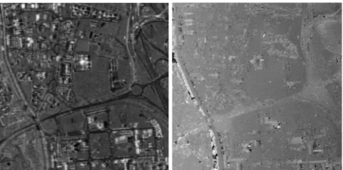
Man-made structures and more generally all features observed at VHR induce rapid height variation with respect to the resolution cell dimension. Since working at full resolution, these rapid height variations combined with phase noise induce in turn high spatial frequencies in the interferometric phase, making the phase unwrapping process potentially difficult even if the ambiguity of altitude is high compared to buildings heights. The generated InSAR DSM contains some small holes made of local DSM areas unwrapped independently. Figure 1 shows the amplitude image of the sample data set in slant range with the derived DSM.
Figure 1: Data set and corresponding seed DSM in slant range After the phase unwrapping process, the seed DSM is still in slant range azimuth geometry. Before being considered as the seed DSM to be iteratively improved, it must be geo-referenced and projected in a convenient geometry.
A convenient geometry is a projection within which further processing for man-made structure detection, localisation and identification will be feasible but also a projection geometry within which SAR scene simulation will stay easy to model. Considering first that man-made structures have no preferential orientation within an observed scene, there is no peculiar advantage of using a specific geographic or cartographic projection rather than another. Therefore, with respect to man-made structure detection, the important point is to work on geo-projected data to get rid of geometrical aspects linked to the slant range geometry. Consequently, working within a given geographic or cartographic projection is of no peculiar importance.
Considering SAR scene simulation, we need a projection geometry allowing to easily model radar wave interaction with the observed scene. Interactions taken into account here are purely geometrical (ray tracing). At the present time, we do not intent to take a local backscattering coefficient into account, even if possibilities to integrate it in the model will be envisioned at each implementation steps.
Based on these considerations, the ground range projection was chosen. This geometry is certainly the simplest to be considered for SAR scene simulation, while, with respect to man-made
structure localization, it is not necessarily the most convenient. Therefore, when performing ground range projection, geo-referencing of each point in terms of longitude and latitude will be saved to allow further projection in any geographic or cartographic reference system.
2.3 Structure definition
Once geo-projected, the seed DSM must be used to define a structure that in turn will be used to model the backscattered SAR signal and simulate the detected SAR scene. Therefore, structure definition depends mainly on the way the simulation process is envisioned. The basic idea is to associate to each point of the DSM, a value that is proportional to the backscattered energy, giving then a peculiar weight to each point. Next, this map of backscattered energy will simply be back-projected in slant range to generate a simulated image. In a first approach, we simply aimed at considering non-coherent dihedral reflection as the main backscattering process to be taken into account.
2.3.1 Dihedral structures: Once more, for the sake of
simplicity and in order to allow us to first perform a proof of concept, we choose to use directly the DSM as the structure itself. Simply, two consecutive heights are used to define a dihedral. The DSM is considered sequentially, azimuth lines by azimuth lines, and within a line, heights are considered sequentially with increasing ground range. If a given height is greater than the preceding one, a dihedral structure can be defined (fig 2).
Figure 2: DSM height interpretation
The part of the incident beam intercepted by a dihedral structure will be fully backscattered toward the beam source. Therefore, the backscattered energy will be proportional to the square of the aperture of the considered dihedral structure; the aperture being the hypotenuse of the illuminated part of the dihedral. Any entering beam in the dihedral follows an optical path of the same length. Therefore, all entering beams will be imaged as localized at the phase centre of the dihedral. Since we are working azimuth lines by azimuth lines, our basis structure is defined in 2D and the phase centre is localized at the intersection of the local horizontal and the local vertical of the considered point.
If we consider two consecutive points of our DSM along a ground range line having respectively heights hi-1 and hi, a
dihedral structure will basically be defined if hi > hi-1; its phase
centre will be localized at ground range coordinate of hi with
local height hi-1 and have a weight proportional to its aperture.
2.3.2 Overestimation: Normally, the aperture of a dihedral
should be computed taking into account shadowing of preceding dihedrals, if any, and be computed with respect to the height difference or with respect to the base, whatever the one is limiting the aperture the first.
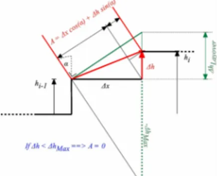
At the present time, we decided to compute the aperture in the simplest way possible to rapidly have a functioning iterative process. Improvements of the structure model will be considered at a later stage. Therefore, apertures are computed directly from the local height difference and from the local incidence angle, not taking into account the base of the dihedral (fig. 3). This can lead to an overestimation of the dihedral aperture.
Figure 3: Basic model of dihedral back-scattering
2.3.3 Dihedral aperture / surface scattering limit: If
dihedral backscattering process may be considered as predominant in the presence of man-made structures in terms of backscattered energy, surface scattering must also be taken into account for open areas that are also well present at VHR. Considering only dihedral backscattering process tends to segment the structure; each time a local height is lower than the preceding one, the aperture, and so the backscattered energy, will be considered as null.
Therefore, we determined a simple height variation limit above which, we consider that dihedral backscattering process occurs and below which, surface backscattering is taking place. The chosen limit is simply the one inducing layover. If the local height difference induces layover, we consider that we have to deal with a dihedral structure, if not, we consider we have to deal with an elementary surface (fig. 4 & 5).
Figure 4: Dihedral structure – surface scattering limit Above the layover limit, the weight of a point will be calculated as its dihedral aperture. Below this limit, surface scattering will be considered.
Figure 5: Surface scattering component
In case of surface scattering, not taking into account a specific local backscattering coefficient, the backscattered energy is taken as proportional to the beam section intercepted by the considered pixel. In place of dihedral aperture, we can thus speak in terms of pixel aperture (fig. 5).
As depicted in figure 5, the intercepted beam section will decrease with the height variation between two pixels up to zero when the shadowing limit is reached.
In terms of backscattered energy, surface backscattering process has a much lower weight than dihedral reflection. Therefore, in practice, a fix coefficient will be applied between both aperture types. At this level, a local backscattering coefficient and/or an emission diagram at pixel level depending on the local slope and on the local incidence should be considered as supplementary weighting factors.
It follows that for a given DSM we define a structure that allows taking into account two backscattering process: dihedral and surface, each with a different weight. Once again, for the sake of simplicity, the current model attributes the computed pixel aperture to the point located at the current position i with height hi as if the point was a phase centre, even if considering surface
scattering.
Consequently, our model defines only point scatterers located on a ground range – azimuth mesh for which height are issued from the projected DSM that must be updated and improved iteratively. At each of these point scatterer position, we will consider we have a point scatterer response whose relative intensity will be determined by the computed aperture.
3. BACK AND FORTH REFERENCING PROCESS
The back and forth referencing and projection processes we have implemented were specifically developed for space-borne sensors. Therefore, no flight motion compensation is considered here. Referencing is thus deduced considering an analytical trajectory of the sensor on its orbit, a fix Doppler cone for the whole scene and a reference geoid (WGS84).
3.1 Ground range referencing
Existing geo-referencing processes allows finding geocentric Cartesian coordinates of a given point in slant range coordinate of know height above the geoid. This geocentric coordinate can then be translated in geodetic coordinate and converted in longitude latitude on the considered datum. Therefore, there is an analytical link between the slant range coordinates of a point of known altitude and its coordinate in a geocentric Cartesian system or in a given cartographic system.
The ground range coordinate of a point given in slant range is defined as the length of a curve segment, which is the intersection between the chosen geoid and the Doppler cone, the length being calculated through integration from the minimum slant range point to the considered point. This integration makes the reverse calculation complicate. Therefore, in the process of calculating the ground range coordinate of a point, this latter one is first geo-referenced on the considered geoid, in longitude - latitude coordinate. This allows building a map linking ground range coordinates with geographical coordinates. This map is then fitted by a second order polynomial for both the longitude and the latitude.
3.2 Slant range referencing
To complete the back and forth projection process, we also need a computational way to reference a point, given in ground range coordinate, back to slant range coordinate. We simply use the second order polynomial linking a ground range position to its longitude – latitude coordinates to find back its geographical position. These geographical coordinates are then converted in Cartesian coordinates in the Earth center coordinate system and the range is derived computing the distance between the position of the sensor on its orbit and the Cartesian coordinate of the considered point.
Special attention was drawn to this back and forth referencing process to ensure reliability and accuracy in accordance with VHR context. In practice, mathematically speaking, the referencing process can easily reach centimeter precision.
4. SAR SCENE SIMULATION 4.1 From aperture to simulated intensity
As explained previously, from a DSM projected in ground range, we build a structure allowing to define either dihedral or surface backscattering. To each point on the ground range sampling grid, we associate what we have called an aperture, which is an evaluation of the incident energy intercepted by the dihedral or the considered surface element. Therefore, from a DSM, we build what might be called an aperture map.
Each point of the ground range mesh is thus considered as a point scatterer to which is associated a point scatterer response backscattering an energy proportional to the incident one. The ground range mesh is then referenced back in slant range and the corresponding projection map is built. For each destination point in slant range, the projection map contains the coordinates of all intervening points in ground range coordinate. Intervening points are those that have to be taken into account to extrapolate the projected value at the considered slant range – azimuth position. After this step, we know the location of the centre of each intervening point scatterer response with respect to a given slant range –azimuth position.
The pixel at that position receives from a given point scatterer response, an energy that is the integral of the impulse response, limited to the slant range pixel area. This integral will be the weight attributed to the contribution of the considered point scatterer response. The simulated energy is obtained summing all contributions of all intervening point scatterers responses for a given slant range pixel.
In SAR, the impulse response or point scatterer response in slant range – azimuth is a sinc-like function generally approximated by a sinc function (Bamler 1993). In terms of energy, we thus deal with a square sinc function and our apertures map in slant range must then be considered as a mesh of square sinc functions of different heights.
In practice, computing the integral of bi-dimensional squared sinc function on a given interval is highly complex. Therefore, we approximate our point scatterer response by a Gaussian having the same width at half maximum. The advantage is that calculating the integral of a bi-dimensional Gaussian on a given interval is straightforward (Fig. 6). One drawback is that strong
side lobes issued from dihedral backscattering process are not modelled.
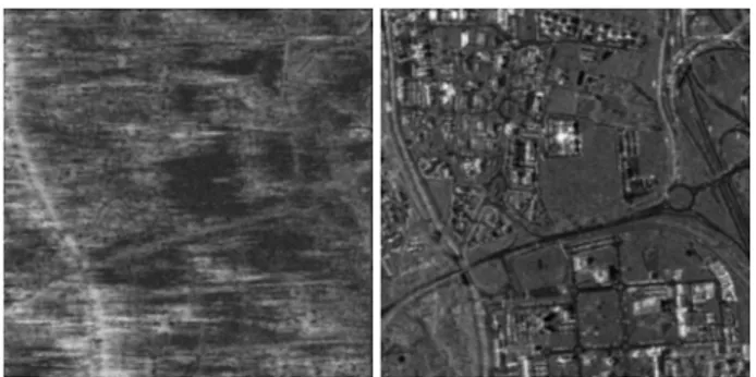
Figure 6: Integration of an approximated point scatterer response limited to a target slant range pixel Figure 7 shows the square root of the simulated image obtained in slant range starting from our seed DSM given in ground range and following the whole procedure described here-above. The real detected SAR image is shown on the right of the figure for qualitative comparison. For the sake of clarity and to improve contrast, the square roots of the simulated intensities are represented.
If, from a macroscopic point of view, similar structures are roughly observable, the simulated image does show a level of details very far from the one of the detected SAR image. Reasons of having apparently so poor results may have three distinct origins: the seed DSM quality, the structure model used for estimating the local backscattered energy and the used parameters.
Figure 7: Simulated SAR scene based on seed DSM structure When projecting the InSAR DSM onto ground range to build the seed DSM, available parameters are on-ground resolution cell dimension, semi-major and semi-minor axis of the ellipse used to find intervening points, weighting method and interpolation method. These parameters have great influence on the smoothing and the quality of the seed DSM.
In the reverse process, when referencing the backscattering structure toward slant range, parameters are the azimuth and slant-range resolution to determine the point scatterer response width, semi-major and semi-minor axis of the ellipse used to find intervening points and the resolution cell dimension of the targeted simulated image.
5. DSM ITERATIVE MODIFICATIONS
At this stage, we have the tools required to link slant range and ground range geometries allowing a back and forth process. The DSM in it self is now in ground range geometry and allows generating a simulated SAR intensity image in slant range geometry to be compared to the really detected one.
For a given point in the simulated image, we have the mapping that lists the points of the seed DSM with their respective weights intervening in the simulation. Conversely, we also have the reverse mapping that, for a given point of the seed DSM, lists points in the simulated image into which the considered DSM point intervene with respective weights. It is this reverse mapping that is used in the DSM modification process.
5.1 Normalisation
To be correct, the simulated image is considered as being an intensity image within an unknown proportionality factor. Before being usable as a valid scene for comparison with the really detected image, the simulated one must be normalized. The normalisation factor is simply the ratio of the integral of the backscattered energy measured in Digital Numbers (DN) in the detected image to the integral of simulated energy.
After normalization, both images represent the same energy globally backscattered by the whole scene, which allows a comparison on a point-by-point basis.
5.2 Improvement criterion
The chosen comparison criterion is simply the local energy ratio. In other words, if the detected energy is higher than the simulated one, the underlying aperture used for the simulation must be increased proportionally.
In the facts, several apertures intervene with different weights in the simulation of a point. Therefore, we work in the reverse way, using the reverse mapping. For a given point of the DSM, the reverse mapping gives us the list of all simulated point into which the considered DSM point intervene with corresponding weights. Consequently, we perform a weighted average of the energy ratios on these simulated and detected points. This weighted average gives us the proportionality factor that should be applied to the underlying aperture.
Whatever the considered backscattering process, apertures are proportional to the local height difference between consecutive points in ground range. Therefore, the proportionality factor can directly be applied to the local height of the DSM under concern.
To summarize, DSM points are corrected sequentially in ground range using a weighted average of intensity ratio calculated on several points in slant range – azimuth. These slant range points are those for which the DSM point under concerns plays a role through the aperture it generates.
5.3 Iterative process
When the corrected DSM is issued, the whole process can be reiterated, starting anew from this new DSM. This latter one will thus be used to compute a new aperture structure and to compute the ground to slant range projection mapping. The mapping will be used in an additive way to generate a simulated SAR intensity image, which, after normalization with respect to the detected one, will be used for DSM improvement. The simulated scene shown on figure 7 can thus be considered as the first iteration of the iterative process described here above.
Figure 8 shows the second iteration of the simulated scene so obtained. The simulated scene appears still of poor quality, but some structures appears more clearly. Corrections with respect
to the first iteration are quite important, and mainly a first segmentation between highly urbanized areas and open areas has roughly been made.
Figure 8: Simulated SAR scene after 2 iterations From a computational point of view, in debug mode, one iteration takes about 4 minute a run for a seed DSM of about 2000x2000 points. This computation time being reasonable, up to 25 iterations have been performed. Figure 9 shows results obtained after 4 and 12 iterations. Figure 10 shows the last iteration along with the really detected scene.
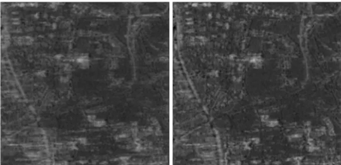
Figure 9: Simulated SAR scene obtained after 4 (left) and 12 (right) iterations
Figure 10: Simulated SAR scene obtained after 25 iterations (left) and really detected one (right)
Clearly, the iterative process converges toward a stable simulation. Qualitatively, convergence appears to be more rapid between the few firsts iterations, while improvement between iteration 12 and 25 becomes less evident. Therefore, the proposed process seams to converge monotonically toward a solution.
It must be noted that the iterative process converges toward a solution that is linked to the underlying aperture model, which in turn, is linked to an improved DSM. Our “improved” DSM is thus “one possible representation of the observed surface”. This possible representation of the observed surface is the one that can be obtained with the developed structure model and using a peculiar set of parameters.
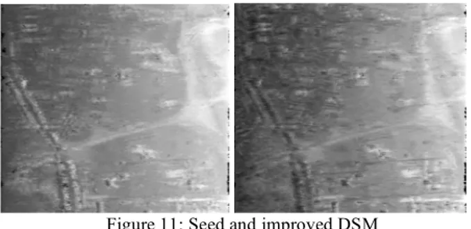
Figure 11 shows in parallel, the seed DSM computed in ground range along with the improved one obtained after 25 iterations.
Figure 11: Seed and improved DSM
While the simulated SAR scene is clearly improved after 25 iterations, improvement is less evident observing the obtained DSM.
Figure 12 represents a DSM sample line, in ground range, before and after improvement. Globally, we observe that the modified DSM appears less noisy and more structured. At this stage, it is difficult to assert if the reached structure is a correct representation of the observed scene and if it can be used in man-made structure detection or identification. But, we can conclude that the achieved structure, together with the proposed model and the used parameter set, allows simulating a SAR intensity image close to the really detected one.
Figure 11: DSM sample line before (green) and after (blue) improvement
Obtaining a DSM representation closer to the observed one will require testing the influence of all parameters as also improving our simplistic model. But, the main point is that we performed a proof of concept of the proposed principle: “Iterative DSM improvement through SAR scene simulation and comparison with observed one”.
Since the proposed method is global and does not require any a priori knowledge on buildings shapes and orientation, it can be envisioned as a first improvement of the DSM to be used in more sophisticated and context-based man-made structure detection techniques.
Nevertheless, if stable, the reached simulated SAR intensity image stays, for the moment, still far from the really detected SAR intensity image. We have well concentrated the energy where it should, but still not with the degree of details offered by the real data. One must thus keep in mind that the obtained improved DSM is just one possible representation of the observed scene. Other representations are possible provided simulation model and set of parameters that are used are optimized
6. CONCLUSIONS
We developed the tools required for simulating a SAR intensity image in slant range geometry starting from a seed DSM given
in ground range and issued from InSAR processing; intensities being solely estimated from local height variations.
Our objective was first to perform a proof of concept, showing that in its principle, it is possible to perform an iterative improvement of a seed DSM by simulation of SAR intensity image in slant range – azimuth projection and comparison with the corresponding detected one. Therefore, we developed a simplistic model allowing to associate a backscattered energy to ground range – azimuth resolution cells with respect to local heights.
Effort was principally put on the reliability and accuracy of back and forth referencing and projection processes.
Clearly, the proof of concept is performed: comparing simulated and detected backscattered energy in slant range allows correcting iteratively the underlying DSM.
The process converges monotonically toward a DSM structure that is thus one possible representation of the observed scene. Monotonic convergence shows that the obtained solution is stable and is, in itself, the result that had to be obtained to validate the proposed iterative process.
Complementary analysis must be performed to assess if the derived DSM can efficiently be used for man-made structures detection.
7. REFERENCES
Balz T, Haala N. (2003), SAR-based 3D reconstruction of
complex urban environments, The International Archives of the
Photogrammetry, Remote Sensing and Spatial Information Sciences, Vol. 34, Part 3/W13, pp.181-185
Balz, T (2006), Automated CAD model-based geo-referencing
for high-resolution SAR data in urban environments. Radar,
Sonar and Navigation, IEE Proceedings - Vol. 153(3), June 2006, pp. 289 - 293
Bamler. R and Schattler B. (1993), SAR data acquisition and
image formation. In: Schreier G. (ed.) SAR geocoding: data and systems.. Wichmann, Karlsruhe, pp. 53-101.
Dupuis X., Dupas J., Oriot H. (2000) 3D extraction from interferometric high resolution SAR images using the RAMSES sensor, PROC. 3rd European Symposium on Synthetic Aperture Radar, EUSAR'2000, München (Germany), VDE, pp. 505-507 Soerger U., Thoennessen U., Stilla U. (2003), Reconstruction of
buildings from interferometric SAR data of built-up areas. The
International Archives of the Photogrammetry, Remote Sensing and Spatial Information Sciences, Vol. 34, Part 3/W13, pp. 59-64
Thiele, A.; Cadario, E.; Schulz, K.; Thonnessen, U.; Soergel, U (2007), Building Recognition From Multi-Aspect
High-Resolution InSAR Data in Urban Areas, IEEE Transactions on
Geoscience and Remote Sensing, 45(11), pp. 3583 - 3593 Tison C., Tupin F., Maitre H. (2007), A fusion scheme for joint
retrieval of urban height map and classification from high-resolution interferometric SAR images, IEEE Tranactions on