1
Nonstationary warm spell frequency analysis integrating climate variability
1and change with application to the Middle East
23 4
Taha B.M.J. Ouarda1, 4, *, Christian Charron1, Kondapalli Niranjan Kumar2, Devulapalli
5
Venkata Phanikumar3, Annalisa Molini4 and Ghouse Basha5
6 7
1Canada Research Chair in Statistical Hydro-Climatology, INRS-ETE, National Institute of 8
Scientific Research, Quebec City (QC), G1K9A9, Canada 9
2Physical Research Laboratory, Ahmedabad, India 10
3Department of Science and Technology, Ministry of Science and Technology, Technology 11
Bhawan, New Delhi 12
4Institute Center for Water and Environment (iWATER), Masdar Institute of Science and 13
Technology, P.O. Box 54224, Abu Dhabi, UAE 14
5National Atmospheric Research Laboratory, Department of Space, Gadanki-517112, India 15 16 17 18 19 20 *Corresponding author: 21 Email: [email protected] 22 Tel: +1 418 654-3842 23 24 25 26 27 April 2019 28 29
2
Abstract
30
The Middle East can experience extended wintertime spells of exceptionally hot weather, which 31
can result in prolonged droughts and have major impacts on the already scarce water resources of 32
the region. Recent observational studies point at increasing trends in mean and extreme 33
temperatures in the Middle East, while climate projections seem to indicate that, in a warming 34
weather scenario, the frequency, intensity and duration of warm spells will increase. The 35
nonstationary warm spell frequency analysis approach proposed herein allows considering both 36
climate variability through global climatic oscillations and climate change signals. In this study, 37
statistical distributions with parameters conditional on covariates representing time, to account for 38
temporal trend, and climate indices are used to predict the frequency, duration and intensity of 39
wintertime warm spells in the Middle East. Such models could find a large applicability in various 40
fields of climate research, and in particular in the seasonal prediction of warm spell severity. Based 41
on previous studies linking atmospheric circulation patterns in the Atlantic to extreme 42
temperatures in the Middle East, we use as covariates two classic modes of ‘fast’ and ‘slow’ 43
climatic variability in the Atlantic Ocean (i.e., the Northern Atlantic Oscillation (NAO) and the 44
Atlantic Multidecadal Oscillation (AMO) respectively). Results indicate that the use of covariates 45
improves the goodness-of-fit of models for all warm spell characteristics. 46
Keywords: Winter warm spell; Nonstationary model; Frequency analysis; Climate index; Climate 47
change; Natural climate variability; Statistical distribution; Middle East. 48
3
1. Introduction
49
In the recent years, an important number of heat waves have been observed around the 50
world resulting in severe adverse societal and economic impacts (Ouarda and Charron, 2018). 51
Examples include Chicago in 1995 (Karl and Knight, 1997), Europe in 2003 (Garcia-Herrera et 52
al., 2010), Greece in 2007 (Founda and Giannakopoulos, 2009), Australia in 2009 (Karoly, 2009), 53
Russia in 2010 (Dole et al., 2012) and Eastern China in 2013 (Sun et al., 2014). While the most 54
immediate adverse impacts of extreme temperatures are those on human health, adverse impacts 55
on natural ecosystems are also important: extreme temperatures and prolonged dry spells induce 56
significant water stress, which brings long-term consequences on vegetation development (Gobron 57
et al., 2005). A number of studies have reported increases in extreme temperature indices since the 58
middle of the 20th century (Alexander et al., 2006; Brown et al., 2008; Perkins et al., 2012; Coumou 59
et al., 2013). It has been argued in several studies that the increase in the reported extreme events 60
is a consequence of global warming (Coumou and Robinson, 2013) which is about 0.5-0.6°C 61
globally since 1951-1980 (Hansen et al., 2012). Many studies point out that, in a context of climate 62
change, the frequency, intensity and duration of extreme heat waves are likely to increase in the 63
future based on climate change scenarios (IPCC, 2012; Coumou and Rahmstorf, 2012; Coumou et 64
al., 2013; Russo et al., 2014; Basha et al., 2017). 65
The Middle East, one of the world most water-stressed regions, is especially sensitive to 66
global warming. The majority of studies on the evolution of climate extremes in the Middle East 67
concluded to an increase in temperature extreme indices and a decrease in precipitation extreme 68
indices during the recent decades (Ouarda et al., 2014). Future climate projections seem also to 69
support an increasing trend in heat extremes over the Middle East. Lelieveld et al. (2016), for 70
4
example, pointed up a consistent positive trend in warm extremes over the region in the CMIP5 71
ensemble models, for both the RCP4.5 and RCP8.5 (business as usual) scenarios. 72
Most of the studies analyzing the extreme temperature regime in the Middle East focus on 73
summer extreme temperatures, due to their immediate impacts on population health (Masselot et 74
al., 2018). However, winter warm spells have also important health, hydrological and 75
environmental impacts. They seriously enhance evapotranspiration and reduce potential 76
groundwater recharge over the water stressed region of the Middle East. Gonzalez et al. (2016) 77
showed that low rainfall, economic and population growth and agricultural development resulted 78
in a dramatic depletion of groundwater resources in the United Arab Emirates (UAE) region during 79
the period 2003-2012. In the context of rapid growth and scarcity of water resources, the Middle 80
East is particularly vulnerable to future climate change (Evans, 2010). Given the evidence of an 81
increasing trend in the observed frequency of occurrence of hot temperature extremes and the 82
projected climate change in the future (IPCC, 2007), the impacts of extreme temperatures have 83
become a growing concern for the Middle East especially during the wet winter season. 84
The study of the physical mechanisms behind heatwaves has been a topic of increased 85
interest (Horton et al., 2016). Perkins (2015) reviewed the physical mechanisms driving heatwaves 86
and identified three major mechanisms. The first one is the presence of a high-pressure synoptic 87
system which results in a stationary system that remains over an area for an abnormally long 88
period. Another driving mechanism is related to the coupling of atmosphere and land surface. 89
Indeed, interactions between air temperature and soil moisture result in important summer 90
temperature variability. The third driving mechanism is associated to climate variability and large-91
scale teleconnections which influence extreme temperatures at a global scale. 92
5
Large scale oscillation patterns have a preponderant influence on the climate of the Middle 93
East. Kumar et al. (2017) demonstrated that the Atlantic and Mediterranean SSTs have a 94
significant influence on winter warm spells over the region. The authors stated that “large and 95
persistent Atlantic SST anomalies modulate the occurrence of the winter warm spells in the Middle 96
East at interannual and decadal scales through the mediation of the Mediterranean SSTs, creating 97
the conditions for the development of extended and persistent anticyclonic structures over the 98
region”. The link between circulation modes and the Middle East climate has been established in 99
many studies (Türkeş and Erlat, 2003; Folland et al., 2009; Erlat and Türkeş, 2013; Donat et al., 100
2014). 101
The Northern Atlantic Oscillation (NAO) is the most frequent mode reported to have an 102
influence on the region (Mann, 2002; Marshall et al., 2001; Cullen et al., 2002; Chandran et al., 103
2016; Naizghi and Ouarda, 2017). The impacts of this pattern are known to be much stronger 104
during the winter season (Marshall et al., 2001; Cullen et al., 2002). Wetter and cooler conditions 105
than normal in the Middle East are associated with positive phases of NAO while drier and warmer 106
than normal conditions are associated with negative phases (Cullen and deMenocal, 2000). 107
Persistent positive values of NAO observed since 1980 may have masked the influence of 108
anthropogenic climate change in the region in recent decades (Mann, 2002). Kumar et al. (2017) 109
also observed that the decadal trends in the occurrence and duration of winter warm spells in the 110
Middle East are significantly correlated with the Atlantic Multidecadal Oscillation (AMO). 111
The influence of other atmospheric circulation indices seems to be less important. The El 112
Niño–Southern Oscillation (ENSO) phenomenon, known to have important impacts on climate 113
around the world, is reported to have a weak influence on temperatures in the region (Halpert and 114
Ropelewski, 1992; Karabörk et al., 2005). However, ENSO is reported to have a significant impact 115
6
on the precipitations in the Arabian Peninsula (Ouarda et al., 2014; Niranjan Kumar et al., 2016), 116
although mainly in terms of moisture advection and precipitable water availability. 117
Statistical methods based on extreme value theory have been used extensively in the 118
analysis of hydrological and weather extremes (Katz et al., 2002; El Adlouni et al., 2007; Ouarda 119
et al., 2019). They have been recently applied to heat waves and warm spells (Furrer et al., 2010; 120
Khaliq et al., 2011; Keellings and Waylen, 2014, 2015; Katz and Grotjahn, 2014; Photiadou et al., 121
2014; Abaurrea et al., 2015). Traditionally, stationarity in time series is assumed and static 122
probability distributions are used. However, in the context of climate warming and under the 123
influence of large scale oscillation patterns, weather extremes are not stationary. One approach to 124
deal with nonstationarity in data samples is to introduce covariates into the parameters of the 125
distribution (e.g. Strupczewski at al., 2001; Khaliq et al., 2006; Ouarda and El Adlouni, 2011). 126
Such distributions are termed conditional because they depend on time-dependent covariates. Such 127
covariates could incorporate trends, cycles or physical variables that can represent atmosphere-128
ocean patterns (Katz et al., 2002; Hundecha et al., 2008). Conditional distributions with a covariate 129
representing the year were extensively used for trend analysis in climate extremes (Kharin and 130
Zwiers, 2005; Brown et al., 2008; Laurent and Parey, 2007; Parey et al., 2007; Keellings and 131
Waylen, 2014). Conditional distributions were also used with climate indices of atmospheric 132
circulation as covariate to evaluate the statistical significance of the influence of large scale 133
atmospheric patterns on climate extremes (Sillmann et al., 2011; Photiadou et al., 2014; Keellings 134
and Waylen, 2015; Grotjahn et al., 2016). 135
In general, models with parameters that are conditional on climate indices may find 136
applications in a number of fields where conditional risk management is required. The severity of 137
warm spells could be predicted for the next season based on actual information about the covariates 138
7
and can help managers with the decision making process. Predictions of warm spell severity could 139
be of interest for managers in various fields including agriculture (Crane et al., 2011), health care 140
(Ebi et al., 2006; Patz et al., 2000; Bayentin et al., 2010) and hydrology (Pulwarty and Melis, 141
2001). It is also possible to predict climate indices in the near future (Sutton et al., 2000; Lee and 142
Ouarda, 2011). Climate forecasting was proven in Jones et al. (2000) to be beneficial for 143
agriculture with decisions conditioned on ENSO phases. A climate forecast information system 144
based on ENSO was developed in the southeastern USA for the management of risk in the field of 145
agriculture (Fraisse et al., 2006). Lowe et al. (2011) reported that heatwave early warning systems 146
have been implemented in 12 European countries to reduce the impacts on public health. 147
In this study, we propose to model the frequency, duration and intensity of wintertime 148
warm spells in the Middle East using nonstationary statistical models with parameters that are 149
conditional on diverse climatic covariates. This approach allows us to account for the effects of 150
global warming and large-scale climate oscillation patterns. The aim of this study is to assess the 151
statistical significance of recent trends caused by both anthropogenic and internal climate 152
variability on wintertime warm spells in the Middles East. Two important climate indices in the 153
Atlantic known to have an influence on wintertime weather patterns in the Middle East, the NAO 154
and the AMO, are used as covariates. The year is used as an additional covariate to represent the 155
temporal trend. Analyses are performed on the regional averaged maximum temperature over a 156
homogenous region in the Middle East. Such approach has never been applied to model climate 157
extremes, including warm spell indices, in the Middle East. While nonstationary models for warm 158
spells have been applied in other regions, models integrating both climate indices and a temporal 159
trend have never been applied. 160
2. Methods
1618 2.1 Statistical modeling of warm spells
162
2.1.1 Modelling of the intensity and frequency 163
In extreme value theory, one approach that has received large popularity consists in 164
extracting the most extreme value within a season and is termed block maxima (BM). Under a 165
wide range of conditions, the distribution of BM can be approximated by the generalized extreme 166
value (GEV) distribution (Coles, 2001). The cumulative distribution function of the GEV is 167 defined by: 168
(
)
(
)
1/ exp 1 , 0 ( ; , , ) exp exp , 0 x GEV x x − − + − = − − − = (1) 169where μ, α > 0 and κ are the location, scale and shape parameters respectively, and 170
/ x
− for 0, − +x for =0 and − −x u / for 0. 171
Another approach, termed peak-over-threshold (POT), consists in extracting exceedances 172
over a sufficiently high threshold. This approach is more appropriate for the analysis of the warm 173
spells in this study because they represent events over a high threshold. An advantage of this 174
approach is that the upper tail of the distribution can be better sampled since more events can be 175
considered during a given season, instead of limiting the sampling to only one peak as in the case 176
of the BM approach (Lang et al., 1999). Another advantage is that the two extreme event 177
components, the rate of occurrence and the intensity of exceedances over the threshold can be 178
modeled separately. The rate of occurrence of rare events is generally modeled by a Poisson(POI) 179
distribution as justified by the law of small numbers, while the intensity of exceedances over a 180
9
sufficiently high threshold is generally modeled by a Pareto (GP) distribution as justified by the 181
theory of extreme values (Ashkar and Ouarda, 1996; Katz and Grotjahn, 2014). This consists in 182
the POI-GP model where intensity and frequency are modeled separately with POI and GP 183
respectively (Katz et al., 2002). 184
The cumulative distribution function of the GP is defined by: 185
(
)
1/ 1 1 , 0 ( ; , , ) 1 exp( ), 0 x u GP x u x u − − + − = − − − = (2) 186where u, > 0 and κ are the threshold, scale and shape parameters respectively, u −x u / 187
for 0, xu for 0. The parameter depends on the threshold and is linked to the 188
parameters of the corresponding GEV distribution by the relation: 189
(
u
)
= +
−
. (3)190
The probability mass function of the POI distribution is defined by: 191
( ; ) n/ !, 1, 2,
Poi N=n =e− n n= . (4)
192
where λ > 0 is the rate parameter and N is the number of crossings of the threshold u. 193
2.1.2 Modelling of the duration 194
It is also common to model the warm spell duration. In a number of studies, the durations 195
of the warm spells were modeled with a geometric distribution (Furrer et al. 2010; Modal and 196
Mujumdar, 2015; Keellings and Waylen, 2014; Wang et al., 2015). The probability mass function 197
of the zero-truncated geometric distribution (GEO) is defined by: 198
10
1
( ; ) (1 )k , 1, 2,
Geo K=k p = −p − p k= (5)
199
where 1/p is the mean duration and K is the length of the warm spell. 200
2.2 Nonstationary models 201
In nonstationary models, distribution parameters are made conditional on time-dependent 202
covariates. The relations between distribution parameters and covariates can take the form of 203
simple linear combinations (El Adlouni et al., 2007; El Adlouni and Ouarda, 2009) or more 204
complex models such as B-splines (Nasri et al., 2013; Thiombiano et al., 2017). When the POI-205
GP model is adopted, usually, the scale parameter ( ) of the GP is made conditional on covariates, 206
the shape parameter (κ) of the GP is kept constant, and the rate parameter (λ) of the POI is made 207
conditional on covariates (Kysely et al., 2010; Modal and Mujumdar, 2015; Thiombiano et al., 208
2018). In this study, the logarithm of the rate parameter in POI can depend linearly or 209
quadratically on a given time-dependent covariate Y : t
210 0 1 ln( )t = +Yt or 2 0 1 2 ln( )t = +Yt+Yt (6) 211
where β are parameters to be estimated. Logarithmic transformations are used to ensure a positive 212
value of the distribution parameters. For GP, the logarithm of the scale parameter can depend 213
linearly or quadratically on the time-dependent covariate Y : t
214 0 1 ln(t)= +Yt or 2 0 1 2 ln(t)= +Yt+Yt . (7) 215
For GEO, the logarithm of the location parameter can depend linearly or quadratically on the time-216
dependent covariate Y : t
11 0 1 ln(pt)= +Yt or 2 0 1 2 ln(pt)= +Yt+Yt . (8) 218
The cases of conditional distributions with 2 and 3 covariates are also considered. Given two 219
additional covariates Z and t W , different combinations of linear and quadratic dependence t
220
relationships between the distribution parameter (t, t or p ) and the covariates t Y and/or t Z t
221
are considered. 222
Three main covariates are used in the nonstationary case: ‘fast’ (subdecadal) and ‘slow’ 223
(multidecadal) climate indices (i.e., NAO and AMO respectively), and Time (represented by the 224
year). The wintertime (NDJFM) averages of NAO and AMO are computed and used as covariates 225
to model the frequency of the winter warm spells. Time is defined by a series of integers 226
incremented from 1 to the number of years in the series, to model the frequency. For the duration 227
and the intensity, each event can be identified precisely in time and thus more precise months can 228
be used to compute the covariates NAO and AMO. A simple method used here consists in taking 229
the average for the three-month period centered on the date of the maximum intensity of each 230
warm spell. Time for the duration and intensity is considered fixed over the warm spell season 231
within a given year but is allowed to shift from one year to another. 232
2.3 Parameter estimation 233
For a given model, the vector of the distribution parameters β is estimated with the 234
maximum likelihood method (ML). For a given probability distribution f, the likelihood function 235
for the sample x ={x ,..., x }1 n is given by: 236 1 ( ; ) n n t t L f x = =
. (9) 23712
Hence, ˆ is the estimator of that maximizes the likelihood function L . n
238
2.4 Model selection and comparison 239
To select the complexity of a model with given covariates, the deviance statistic can be 240
used for model selection as proposed by Coles (2001). Suppose two models M1 and M0, where M0 241
is a subset of M1. The deviance statistic is defined by: 242
1 1 0 0
2{ ( ) ( )}
D= M − M (10)
243
where 1(M and 1) 0(M0) are the maximized values of the log-likelihood for models M1 and M0 244
respectively. It can be proven that D is distributed according to the 2
l
distribution where l is the 245
difference between the dimension of M1 and M0. A test of validity of the model M0 relative to M1 246
is to reject M0 in favor of M1 if D > 2
l
for a given level of significance. 247
To compare the goodness-of-fit of different models, we use the Akaike information 248
criterion (AIC), defined as: 249
AIC= −2ln(Ln) 2+ d, (11)
250
where d is the number of parameters of the model or the length of the vector . This statistic 251
accounts for the goodness-of-fit of the model and also for the parsimony through the parameter k 252
whose value increases with model complexity. 253
2.5 Definition of warm spells 254
There is in general very little consensus and consistency in the literature on how to identify 255
warm spells, and different studies often rely on very different definitions and selection thresholds 256
13
(Perkins and Alexander, 2012; Masselot et al., 2018). The simplest definition is ‘the period of 257
consecutive days with temperature over a given relative or absolute threshold’, which, however, 258
risks to marginalize the role of local climatology (Robinson, 2001). In this study we follow a 259
percentile based criterion similar to the ones proposed by Della-Marta et al. (2007) and Stefanon 260
et al. (2012), where a heat wave is defined as the period of consecutive days where the daily 261
maximum temperature exceeds the long-term (climatological) 90th percentile of daily maximum 262
temperatures. For each day of the year, a 90th percentile is calculated from a sample of 15 days 263
centered on the considered day using data over the whole base period. This is equivalent to the 264
POT approach with a relative threshold dependent on the day of the year. Also, we introduce the 265
additional constraint that both daily maximal and minimal temperatures should exceed the daily 266
maximum and minimum temperatures 90th percentiles. A minimum number of days above the 267
threshold may be considered (e.g. Freychet et al., 2018) or not (Furrer et al., 2010). In this study, 268
a minimum duration is not considered. Declustering is frequently used with the POT approach to 269
avoid consecutive dependent events. A common rule to separate exceedances in clusters is to 270
consider clusters separated by r consecutive values below the threshold as independent (Coles, 271
2001). The choice of r is arbitrary: a larger value ensures the independence but a smaller value 272
reduces the data size. Following the studies of Keellings and Waylen (2014, 2015) on heat waves, 273
r is set to 4 days in this study.
274
Time series for the frequency, duration and intensity of warm spells were computed from 275
the wintertime warm spell events extracted with the method presented above from Middle East 276
temperature data (see Section 3, Data). Here, frequency is defined as the number of warm spell 277
occurrences per winter, the duration is defined in days during a warm spell event and the intensity 278
is defined as the maximum exceedance of the daily maximum temperature during a warm spell 279
14
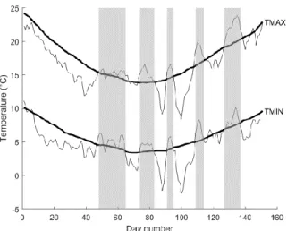
event. The winter period is defined here as the period during the months November through March 280
(NDJFM). Figure 1 presents an example of the daily quantile-threshold approach used to identify 281
warm spells in the study region for the winter of 2009-2010. The 2009-2010 winter was one of the 282
warmest winters on record in the Middle East, thus representing a good benchmark for our method. 283
Figure 1 shows in fact five main significant warm events between November 2009 and March 284 2010. 285
3. Data
286 3.1 Data sources 287Atmospheric temperatures used in this study are obtained from the NCEP/NCAR 288
Reanalysis (Kalnay et al., 1996). Daily maximum and minimum temperatures are available on a 289
Gaussian grid (The latitudinal grid spacing varies to preserve equal areas and is approximately 290
equal to 1.9° while the longitudinal spacing is 1.875°). Data are obtained for the period 1948-2016 291
for grid points over the Middle East and for the extended winter season (November to March, 292
NDJFM). 293
AMO is defined as the anomaly of the area weighted average of the SST over the North 294
Atlantic (between 0-70°N, (Trenberth and Shea, 2006; Peings and Magnusdottir, 2014; Enfield et 295
al., 2001)). It can be obtained from the NOAA Physical Science Division at 296
https://www.esrl.noaa.gov/psd/data/timeseries/AMO/. NAO is based on the surface sea-level 297
pressure difference between the Subtropical (Azores) High and the Subpolar Low. NAO is 298
obtained from the Climate Prediction Center (CPC) at the National Centers for Environmental 299
Prediction (NCEP) at the address: http://www.cpc.ncep.noaa.gov/data/teledoc/nao.shtml. NAO is 300
available from 1950 and AMO from 1948, and both indices are updated monthly. 301
15 3.2 Spatial extent
302
To compute the regional warm spell variables, the daily local maximum and minimum 303
temperatures were averaged over a homogenous region. The definition of the homogenous region 304
for this study is based on the EOF analysis of the winter mean temperature (Abatzoglou et al., 305
2009; Conroy and Overpeck, 2011). The EOF of the mean temperature during the wet season 306
(NDJFM) for the grid points between 10-45°N and 20-65°E were extracted and the orthogonal 307
varimax rotation was applied to the significant EOFs. Rotation of the eigenvectors is usually 308
performed on a subset of the original EOFs in studies using EOF for the identification of the 309
regional patterns of climate variability (White et al., 1991; Fovell and Fovell, 1993; Comrie and 310
Glenn, 1998; Simpson et al., 2005; Abatzoglou et al., 2009; Conroy and Overpeck, 2011). Rotation 311
allows to enhance physical interpretation. The first four principal components were tested for 312
significance on the basis of the scree test (Cattell, 1966). The scree test is a simple method 313
consisting in plotting the eigenvalues versus the rank and identifying changes in slope. 314
There are several methods to identify statistically homogeneous regions using EOFs. They 315
can be defined, for example, by using contours (Comrie and Glenn, 1998), the maximum loading 316
rule (Conroy and Overpeck, 2011) or cluster analysis (Guttman, 1993). Figure 2 presents the region 317
of interest obtained with each one of these methods. They all lead to similar results, highlighting 318
a homogenous region embracing most of the Arabian Peninsula, Levant countries, Turkey, Iraq 319
and Iran. The region delineated using the contour defines the homogenous region used in this 320
study. 321
4. Results
3224.1 Trend and change point analysis 323
16
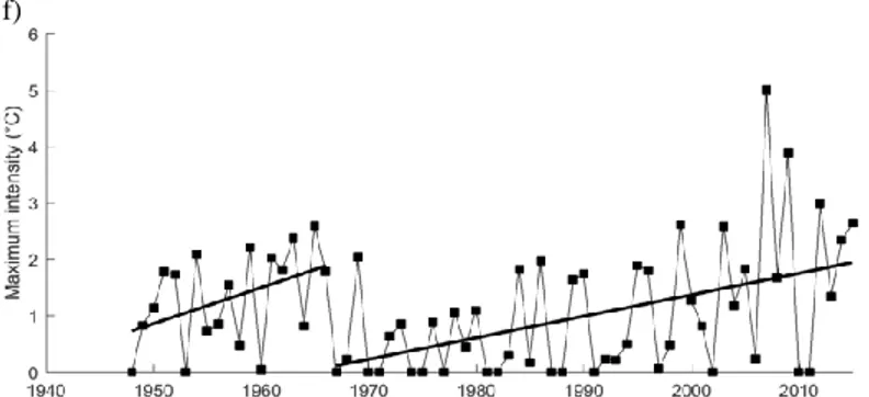
The presence of potential trends and abrupt changes in warm spell characteristics is 324
investigated in this subsection. Specifically, abrupt changes were investigated with a Bayesian 325
multiple change point detection procedure (Seidou et al., 2007; Seidou and Ouarda, 2007). This 326
procedure allows to automatically detect multiple shifts or changes in the trend. The change point 327
detection procedure was applied to the frequency of warm spells and to the following other annual 328
variables computed from the warm spell variables: total duration, mean duration, longest duration, 329
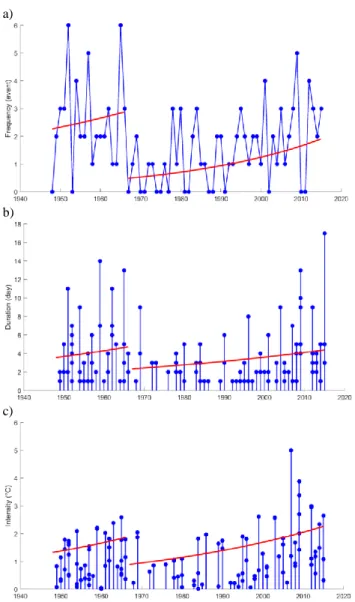
mean intensity and maximum intensity. Annual time series and linear trends for the various 330
delineated segments are presented in Figure 3. A change point is detected in all cases during the 331
late 1960s except for the mean intensity. Such a shift is coherent with the shift observed during the 332
same period in the characteristics of global atmospheric circulation by Baines and Folland (2007). 333
These authors highlighted how, in particular, such shift was evident in Greenland annual mean 334
temperature patterns, eventually leading to similar changes in SST in the higher latitudes of the 335
North Atlantic. The main cause of the late 1960s climate shift could also be found in the North 336
Atlantic, and derives from a reduction in the northward oceanic heat flux from the North Atlantic 337
thermohaline circulation in the 1950s to 1970s. For all variables with a change point during the 338
late 1960s, trends have since increased. 339
Trends in the model parameters t, p and t t are analyzed here as these parameters allow 340
to infer on trends in the frequency, duration and intensity of warm spells. In Figure 4, trends in the 341
model parameters t, p and t t before and after the year 1967 are also superimposed on the 342
graphs of the time series of warm spell frequency, duration and intensity respectively. The year 343
1967 is selected to represent the shift observed in the heat spell features during the late 1960s and 344
corresponds to the shift obtained for the warm spell frequency with the change point detection 345
procedure (see Figure 3a). To compute trends in the model parameters, the nonstationary POI, 346
17
GEO and GP models with Time used as a covariate are fitted to the time series before and after 347
the shift. Increasing trends are observed in the time series, since the shifts are observed, for every 348
warm spell variable, and these trends are found to be statistically significant based on the deviance 349
statistic. It is also worth noting that the longest warm spell happened during the winter season of 350
2015-2016, which is the last year of record, and the most intense warm spell occurred during the 351
winter season of 2007-2008, to coincide with one of the most extended and intense mega-droughts 352
on record over the region (Barlow et al., 2016; Gleick, 2014). 353
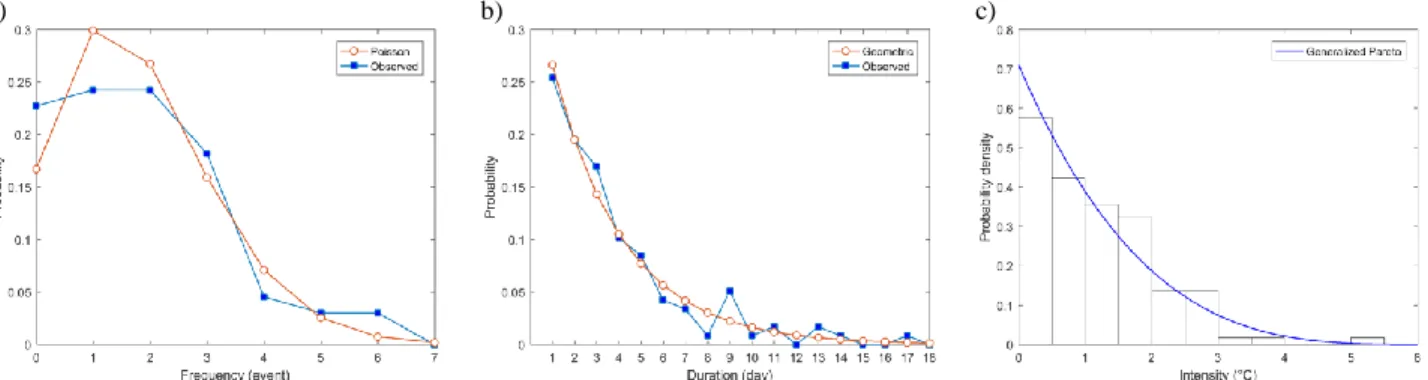
4.2 Validation of the probability functions 354
In this subsection, the choices of the different probability functions used to model warm 355
spell variables are validated. Figure 5 compares the theoretical probability distributions inferred 356
from data with the corresponding observed relative frequencies for the frequency, duration and 357
intensity of winter warm spells. These graphs suggest that the selected theoretical probability 358
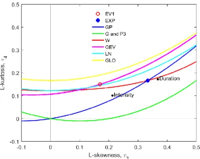
distributions are suitable to model the warm spell variables. To confirm the suitability of the 359
selected theoretical distributions, Figure 6 presents the L-moment ratio diagram with the location 360
of the sample L-moments of the variables’ duration and intensity. The sample L-moments of the 361
duration and intensity are located respectively near the theoretical curve of the GP and the 362
theoretical point of the exponential distribution (the continuous probability distribution analogous 363
to the GEO). The sample L-moments of the frequency are not shown in the diagram because the 364
POI theoretical distribution is not usually represented in moment ratio diagrams, and therefore 365
there is missing information in the literature about the location of this distribution. 366
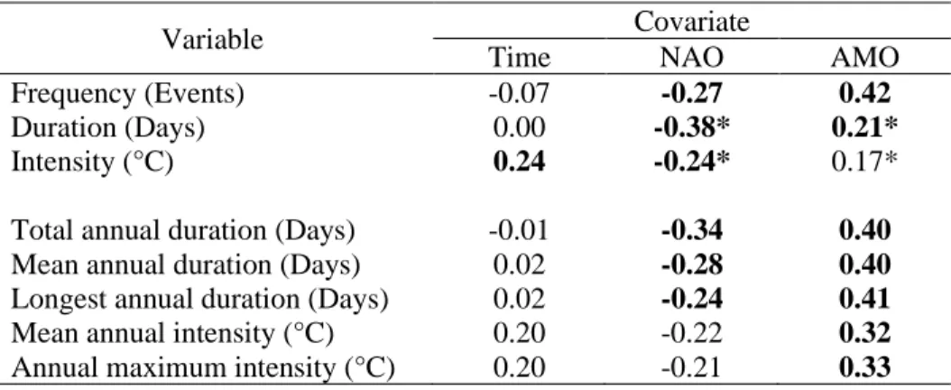
4.3 Relationship of warm spell variables with climate indices 367
18
Relationships of climate indices with the warm spell variables are evaluated in this 368
subsection. Table 1 presents the correlations between the warm spell variables and the covariates 369
Time, NAO and AMO. The majority of the variables are significantly correlated with NAO and 370
AMO. Correlations with Time are weak in general except for the intensity and the mean and annual 371
maximum intensity. However, the extended period of high values observed in the series prior to 372
the shift during the late 1960s masks the positive significant trends observed after the shift. 373
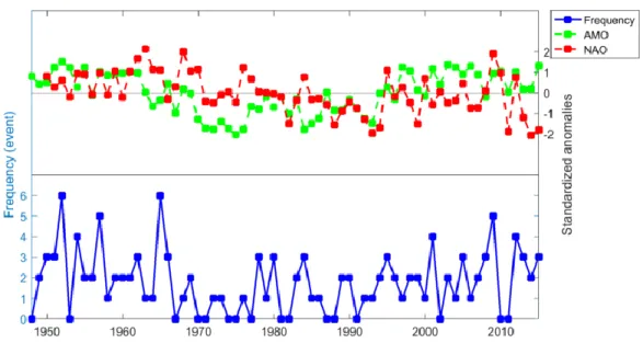
Figure 7 reports on the same graph the frequency of warm spells, the inverse of the 374
standardized wintertime NAO and the standardized wintertime AMO. Correlations between the 375
climate indices and the frequency are clearly visible. For instance, the prolonged period of high 376
frequency of 1950-1966 corresponds to a prolonged period of higher than normal AMO and the 377
prolonged period of low frequency of 1967-1977 corresponds to a prolonged period of lower than 378
normal AMO, pointing out a clear multidecadal signature in the time evolution of Middle Eastern 379
winter warm spells. The correlation between the two climate indices for wintertime is rather weak 380
with a value of -0.16 during the record period. This low value implies that these two covariates 381
can be included together in a nonstationary model and improve the goodness-of-fit compared to 382
models using the climate indices separately. 383
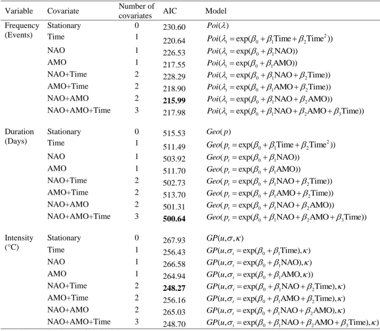
4.4 Nonstationary modelling 384
The nonstationary models presented in Section 2.2 were applied to the regionally averaged 385
time series of warm spell characteristics including each one of the selected covariates, all the 386
combinations of two covariates and the three selected covariates together. The analyses were 387
applied to the period 1950-2016 for which both climate indices are available. Table 2 presents the 388
optimal models obtained according to the test of the deviance for each warm spell variable and 389
19
each possible configuration of the covariates. The values of the AIC statistic obtained for each 390
optimal model are also presented and are used to compare goodness-of-fits. Here, we can observe 391
that the goodness-of-fit obtained for models with one or more covariates is systematically higher 392
than the one for the stationary model for a given variable. For models including one covariate, best 393
fits are obtained with AMO for the frequency, NAO for the duration and Time for the intensity. 394
This suggests that the climate indices have more impact on the frequency and the duration than the 395
temporal trend, while the temporal trend has more impact on the intensity than the climate indices. 396
From a climate dynamics point of view, this is like saying that large-scale climate oscillations 397
basically pose the conditions to trigger the onset of winter warm spells, while the intensity of the 398
different events may be determined by more local processes like land-atmosphere interactions and 399
feedbacks. 400
For models including two covariates, the overall best goodness-of-fit statistic is obtained 401
with NAO+AMO for the frequency, and NAO+Time for the duration and the intensity. Adding 402
Time to either NAO or AMO (NAO+Time or AMO+Time) does not improve the corresponding 403
model which includes only NAO or AMO for the frequency. For the duration, adding Time to 404
NAO improves the goodness-of-fit while it is not the case for AMO+Time. For the intensity, a 405
larger impact on the goodness-of-fit with NAO+Time than with AMO+Time is observed, where 406
the AIC value passes from 266.58 to 248.27 for NAO+Time compared to NAO only. For the 407
intensity, models that include Time (NAO+Time or AMO+Time) outperform models that include 408
only one climate index (NAO and AMO) and the model including both climate indices 409
(NAO+AMO). This result indicates that there is a strong temporal trend in the intensity which is 410
not explained by the climate indices. Including both NAO and AMO (NAO+AMO) in a model 411
generally improves the goodness-of-fit compared to models using each climate index separately. 412
20
This implies that both indices are somehow complementary and that it is of interest to use both 413
indices together. Using the three covariates together (NAO+AMO+Time) leads to models with 414
some of the best goodness-of-fit statistics for each variable: the third, the first and the second 415
overall best ranks are obtained respectively for the frequency, duration and intensity. 416
It can be concluded from these results that the variability in the warm spell variables is 417
partly explained by climate indices. The temporal trend associated with the global warming has 418
also a great impact on the variability of the variables and this is particularly true for the intensity. 419
The fact that the inclusion of Time with AMO has a weaker influence on the goodness-of-fit than 420
the inclusion of Time with NAO is probably caused by the positive trend observed in AMO since 421
the 1970s, and is coherent with global warming (see Figure 7). Indeed, it is known that AMO is a 422
combination of a forced global warming trend with a distinct local multidecadal oscillation that 423
arose from internal variability (Ting et al., 2009). 424
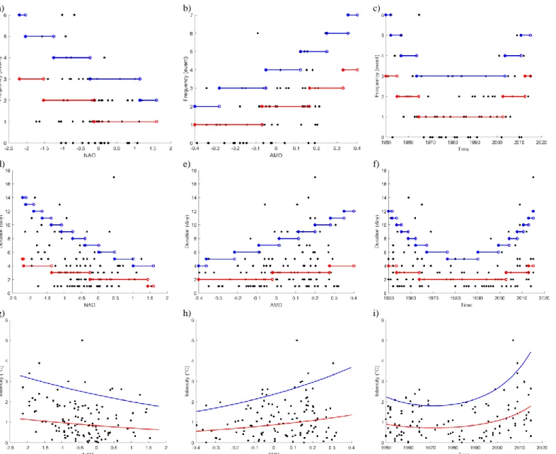
Figure 8 illustrates the quantiles corresponding to nonexceedance probabilities p = 0.5 and 425
0.9 for warm spell variables obtained with the nonstationary models including one covariate. 426
Quantiles of each variable are presented on separate graphs as a function of the covariates NAO, 427
AMO and Time. The quantiles corresponding to frequency and duration are represented with step 428
functions because of the discrete nature of the probability distributions POI and GEO. It is clear 429
from Figures 8a-8f that the relationships of the quantiles with Time are rather unrealistic for the 430
frequency and duration. The quadratic model was selected in both cases, resulting in decreasing 431
trends during the period 1950-1970 and increasing trends during the period 1990-2015. These 432
trends are strongly influenced by climate oscillation patterns for which no index is included in the 433
model in this case. For the duration, there is an outlier for an event happening during the winter 434
2015-2016 where for the longest duration observed, the value of NAO is in the middle range. 435
21
Figures 9-11 present the quantiles corresponding to the nonexceedance probability p = 0.9 436
obtained with the nonstationary models including two covariates for the frequency, duration and 437
intensity respectively. For each variable, the optimal models obtained with the three possible 438
combinations of two covariates are graphically represented. Quantiles are illustrated in two 439
different ways: with 2-dimensional graphs where the quantiles are represented using colors (a, c, 440
e), and with 3-dimensional graphs (b, d, f) where the frequency is shown as a function of the two 441
covariates. Quantiles corresponding to the frequency and duration are also represented here with 442
step functions for the same reasons. The figures corresponding to models with both NAO and 443
AMO illustrate well the combined effect of both climate indices: when both covariates have 444
extreme values of opposite signs, the quantiles are extreme (either very strong or very weak). For 445
the frequency and duration, strong relationships with climate indices and slight temporal trends 446
are noticed in Figures 9-10. In the case of models with covariates NAO+Time, increasing temporal 447
trends are observed, and in the case of models with covariates AMO+Time, decreasing temporal 448
trends are observed. These decreasing temporal trends for AMO+Time are counterintuitive in a 449
context a global warming. However, the temporal trends in models with AMO+Time are not 450
significant for the frequency and duration as the goodness-of-fit of models with only AMO is more 451
optimal in both cases (see Table 2). In the case of the intensity, strong relationships with climate 452
indices in conjunction with strong positive temporal trends are noticed, in agreement with what 453
was observed previously. 454
5. Conclusions
455In this study, temperatures during the winter season (NDJFM) were aggregated over a 456
homogenous region over the Middle East to obtain regional daily average minimum and maximum 457
temperatures. Warm spell events were identified from these regionally averaged time series and 458
22
the warm spell frequency, duration and intensity were obtained. To account for the 459
nonstationarities associated with global warming and climate oscillation patterns, statistical 460
distributions with parameters conditional on time-dependent covariates were used to model the 461
wintertime warm spell characteristics in the region. The covariates of the model include two 462
important climate indices, the NAO and the AMO, explaining temperature variability in the Middle 463
East, and Time as a covariate representing the temporal trend related to global warming. 464
Results show that the inclusion of any one of the covariates improves the goodness-of-fit 465
of the stationary model. For models with only one covariate, the best fit is obtained with AMO for 466
the frequency, NAO for the duration and Time for the intensity. This may indicate that the 467
influence of climate oscillation patterns is more important than the influence of the temporal trend 468
for the frequency and the duration. On the other hand, the temporal trend influences the intensity 469
more than do climate indices. Including both climate indices generally improved the goodness-of-470
fit as compared to the models which include only one climate index. These results advocate for 471
the use of both climate indices at the same time. The overall best goodness-of-fits are obtained 472
with NAO and AMO for the frequency, NAO, AMO and Time for the duration, and NAO and 473
Time for the intensity. These results show the importance of considering the combined effect of 474
the temporal trend caused by global warming and climate oscillation patterns in statistical models 475
used for the prediction of extreme climatic variables. 476
The nonstationary statistical models used in this study can find application in a number of 477
different fields where conditional risk management is required, such as agriculture, public health 478
management and hydrology. For example, seasonal predictions of the diverse climate indices can 479
be used to model warm spell quantiles. More optimal management decisions can then be made 480
before the start of the next season based on that information. 481
23 482
Acknowledgments
483Financial support for the present study was provided by the Natural Sciences and Engineering 484
Research Council of Canada (NSERC). Daily temperature data used in this study comes from the 485
NCEP/NCAR Reanalysis database and was downloaded from the NOAA’s Earth System Research 486
Laboratory (https://www.esrl.noaa.gov/psd/data/gridded/data.ncep.reanalysis.html). Sea surface 487
temperature data comes from the Met Office Hadley Centre (downloaded at 488
http://hadobs.metoffice.com/hadisst/). Data for the climate indices AMO and NAO is updated and 489
available respectively from the NOAA ESRL Physical Science Division (PSD) 490
(https://www.esrl.noaa.gov/psd/data/timeseries/AMO/) and the NCEP Climate Prediction Center 491
(CPC) (http://www.cpc.ncep.noaa.gov/data/teledoc/nao.shtml). The authors are grateful to the 492
Executive Editor, Dr. Jian Lu, and to two anonymous reviewers for their comments which helped 493
improve the quality of the manuscript. 494
24
References
496
Abatzoglou JT, Redmond KT, Edwards LM (2009) Classification of Regional Climate 497
Variability in the State of California. Journal of Applied Meteorology and Climatology 498
48:1527-1541. doi:10.1175/2009JAMC2062.1 499
Abaurrea J, Asín J, Cebrián AC (2015) Modeling and projecting the occurrence of bivariate 500
extreme heat events using a non-homogeneous common Poisson shock process. Stochastic 501
Environmental Research and Risk Assessment 29:309-322. doi:10.1007/s00477-014-0953-502
9 503
Alexander LV et al. (2006) Global observed changes in daily climate extremes of temperature 504
and precipitation. Journal of Geophysical Research: Atmospheres 111. 505
doi:10.1029/2005JD006290 506
Ashkar F, Ouarda TBMJ (1996) On some methods of fitting the generalized Pareto distribution. 507
Journal of Hydrology 177:117-141. doi:10.1016/0022-1694(95)02793-9 508
Baines PG, Folland CK (2007) Evidence for a Rapid Global Climate Shift across the Late 1960s. 509
Journal of Climate 20:2721-2744. doi:10.1175/JCLI4177.1 510
Barlow M, Zaitchik B, Paz S, Black E, Evans J, Hoell A (2016) A Review of Drought in the 511
Middle East and Southwest Asia. Journal of Climate 29:8547-8574. doi:10.1175/jcli-d-13-512
00692.1 513
Basha G, Kishore P, Ratnam MV, Jayaraman A, Agha Kouchak A, Ouarda TBMJ, Velicogna I 514
(2017) Historical and projected surface temperature over India during the 20th and 21st 515
century. Scientific Reports 7:2987. doi:10.1038/s41598-017-02130-3 516
Bayentin L, El Adlouni S, Ouarda TB, Gosselin P, Doyon B, Chebana F (2010) Spatial 517
variability of climate effects on ischemic heart disease hospitalization rates for the period 518
1989-2006 in Quebec, Canada. International Journal of Health Geographics 9:1-10. 519
doi:10.1186/1476-072x-9-5 520
Brown SJ, Caesar J, Ferro CAT (2008) Global changes in extreme daily temperature since 1950. 521
Journal of Geophysical Research: Atmospheres 113. doi:10.1029/2006JD008091 522
Cattell RB (1966) The Scree Test For The Number Of Factors. Multivariate Behavioral Research 523
1:245-276. doi:10.1207/s15327906mbr0102_10 524
Chandran A, Basha G, Ouarda TBMJ (2016) Influence of climate oscillations on temperature 525
and precipitation over the United Arab Emirates. International Journal of Climatology 526
36:225-235. doi:10.1002/joc.4339 527
25
Coles S (2001) An introduction to statistical modeling of extreme values. Springer, London. 528
Comrie AC, Glenn EC (1998) Principal components-based regionalization of precipitation 529
regimes across the southwest United States and northern Mexico, with an application to 530
monsoon precipitation variability. Climate Research 10:201-215. doi:10.3354/cr010201 531
Conroy JL, Overpeck JT (2011) Regionalization of Present-Day Precipitation in the Greater 532
Monsoon Region of Asia. Journal of Climate 24:4073-4095. doi:10.1175/2011jcli4033.1 533
Coumou D, Rahmstorf S (2012) A decade of weather extremes. Nature Climate Change 2:491-534
496. doi:10.1038/nclimate1452 535
Coumou D, Robinson A (2013) Historic and future increase in the global land area affected by 536
monthly heat extremes. Environmental Research Letters 8:034018. doi:10.1088/1748-537
9326/8/3/034018 538
Coumou D, Robinson A, Rahmstorf S (2013) Global increase in record-breaking monthly-mean 539
temperatures. Climatic Change 118:771-782. doi:10.1007/s10584-012-0668-1 540
Crane TA, Roncoli C, Hoogenboom G (2011) Adaptation to climate change and climate 541
variability: The importance of understanding agriculture as performance. NJAS - 542
Wageningen Journal of Life Sciences 57:179-185. doi:10.1016/j.njas.2010.11.002 543
Cullen HM, deMenocal PB (2000) North Atlantic influence on Tigris–Euphrates streamflow. 544
International Journal of Climatology 20:853-863. doi:10.1002/1097-545
0088(20000630)20:8<853::AID-JOC497>3.0.CO;2-M 546
Cullen HM, Kaplan A, Arkin PA, deMenocal PB (2002) Impact of the North Atlantic Oscillation 547
on Middle Eastern Climate and Streamflow. Climatic Change 55:315-338. 548
doi:10.1023/a:1020518305517 549
Della-Marta PM, Haylock MR, Luterbacher J, Wanner H (2007) Doubled length of western 550
European summer heat waves since 1880. Journal of Geophysical Research: Atmospheres 551
112. doi:10.1029/2007JD008510 552
Dole R et al. (2011) Was there a basis for anticipating the 2010 Russian heat wave? Geophysical 553
Research Letters 38. doi:10.1029/2010GL046582 554
Donat M et al. (2014) Changes in extreme temperature and precipitation in the Arab region: 555
long‐term trends and variability related to ENSO and NAO. International Journal of 556
Climatology 34:581-592. doi:10.1002/joc.3707 557
Ebi KL, Lewis ND, Corvalan C (2006) Climate variability and change and their potential health 558
effects in small island states: information for adaptation planning in the health sector. 559
Environmental Health Perspectives 114:1957-1963. doi:10.1289/ehp.8429 560
26
El Adlouni S, Ouarda TBJM, Zhang X, Roy R, Bobee B (2007) Generalized maximum 561
likelihood estimators for the nonstationary generalized extreme value model. Water 562
Resources Research 43:W03410. doi:10.1029/2005WR004545 563
El Adlouni S, Ouarda TBMJ (2009) Joint Bayesian model selection and parameter estimation of 564
the generalized extreme value model with covariates using birth-death Markov chain 565
Monte Carlo. Water Resources Research 45:W06403. doi:10.1029/2007wr006427 566
Enfield DB, Mestas-Nuñez AM, Trimble PJ (2001) The Atlantic Multidecadal Oscillation and its 567
relation to rainfall and river flows in the continental U.S. Geophysical Research Letters 568
28:2077-2080. doi:10.1029/2000GL012745 569
Erlat E, Türkeş M (2013) Observed changes and trends in numbers of summer and tropical days, 570
and the 2010 hot summer in Turkey. International Journal of Climatology 33:1898-1908. 571
doi:10.1002/joc.3556 572
Evans JP (2010) Global warming impact on the dominant precipitation processes in the Middle 573
East. Theoretical and Applied Climatology 99:389. doi:10.1007/s00704-009-0151-8 574
Folland CK, Knight J, Linderholm HW, Fereday D, Ineson S, Hurrell JW (2009) The Summer 575
North Atlantic Oscillation: Past, Present, and Future. Journal of Climate 22:1082-1103. 576
doi:10.1175/2008jcli2459.1 577
Founda D, Giannakopoulos C (2009) The exceptionally hot summer of 2007 in Athens, Greece 578
— A typical summer in the future climate? Global and planetary change 67:227-236. 579
doi:10.1016/j.gloplacha.2009.03.013 580
Fovell RG, Fovell M-YC (1993) Climate Zones of the Conterminous United States Defined 581
Using Cluster Analysis. Journal of Climate 6:2103-2135. doi:10.1175/1520-582
0442(1993)006<2103:czotcu>2.0.co;2 583
Fraisse CW et al. (2006) AgClimate: A climate forecast information system for agricultural risk 584
management in the southeastern USA. Computers and Electronics in Agriculture 53:13-27. 585
doi:10.1016/j.compag.2006.03.002 586
Freychet N, Sparrow S, Tett SFB, Mineter MJ, Hegerl GC, Wallom DCH (2018) Impacts of 587
Anthropogenic Forcings and El Niño on Chinese Extreme Temperatures. Advances in 588
Atmospheric Sciences 35:994-1002. doi:10.1007/s00376-018-7258-8 589
Furrer EM, Katz RW, Walter MD, Furrer R (2010) Statistical modeling of hot spells and heat 590
waves. Climate Research 43:191-205. doi:10.3354/cr00924 591
García-Herrera R, Díaz J, Trigo R, Luterbacher J, Fischer E (2010) A review of the European 592
summer heat wave of 2003. Critical Reviews in Environmental Science and Technology 593
40:267-306. doi:10.1080/10643380802238137 594
27
Gleick PH (2014) Water, Drought, Climate Change, and Conflict in Syria. Weather, Climate, and 595
Society 6:331-340. doi:10.1175/WCAS-D-13-00059.1 596
Gobron N et al. (2005) The state of vegetation in Europe following the 2003 drought. 597
International Journal of Remote Sensing 26:2013-2020. 598
doi:10.1080/01431160412331330293 599
Gonzalez R, Ouarda T, Marpu P, Allam M, Eltahir E, Pearson S (2016) Water Budget Analysis 600
in Arid Regions, Application to the United Arab Emirates. Water 8:415. 601
doi:10.3390/w8090415 602
Grotjahn R et al. (2016) North American extreme temperature events and related large scale 603
meteorological patterns: a review of statistical methods, dynamics, modeling, and trends. 604
Climate Dynamics 46:1151-1184. doi:10.1007/s00382-015-2638-6 605
Guttman NB (1993) The Use of L-Moments in the Determination of Regional Precipitation 606
Climates. Journal of Climate 6:2309-2325. doi:10.1175/1520-607
0442(1993)006<2309:tuolmi>2.0.co;2 608
Halpert MS, Ropelewski CF (1992) Surface Temperature Patterns Associated with the Southern 609
Oscillation. Journal of Climate 5:577-593. doi:10.1175/1520-610
0442(1992)005<0577:stpawt>2.0.co;2 611
Hansen J, Ruedy R, Sato M, Lo K (2010) Global Surface Temperature Change. Reviews of 612
Geophysics 48. doi:10.1029/2010RG000345 613
Horton, R.M., Mankin, J.S., Lesk, C., Coffel, E., Raymond, C., 2016. A Review of Recent 614
Advances in Research on Extreme Heat Events. Current Climate Change Reports: 1-18. 615
doi:10.1007/s40641-016-0042-x 616
Hundecha Y, St-Hilaire A, Ouarda TBMJ, El Adlouni S, Gachon P (2008) A Nonstationary 617
Extreme Value Analysis for the Assessment of Changes in Extreme Annual Wind Speed 618
over the Gulf of St. Lawrence, Canada. Journal of Applied Meteorology and Climatology 619
47:2745-2759. doi:10.1175/2008jamc1665.1 620
IPCC (2007) IPCC, 2007: Summary for Policymakers. In: Climate Change 2007: The Physical 621
Science Basis. Contribution of Working Group I to the Fourth Assessment Report of the 622
Intergovernmental Panel on Climate Change [Solomon, S., D. Qin, M. Manning, Z. Chen, 623
M. Marquis, K.B. Averyt, M.Tignor and H.L. Miller (eds.)]. Cambridge University Press, 624
Cambridge, United Kingdom and New York, NY, USA. 625
IPCC (2012) Managing the risks of extreme events and disasters to advance climate change 626
adaptation. A special report of Working Groups I and II of the Intergovernmental Panel on 627
Climate Change (IPCC) [Field, C. B., V. Barros, T. F. Stocker, D. Qin, D. J. Dokken, K. L. 628
28
Ebi, M. D. Mastrandrea, K. J. Mach, G.-K. PLattner, S. K. Allen, M. Tignor, and P. M. 629
Midgley (eds.)]. Cambridge University Press, Cambridge, United Kingdom and New York, 630
NY, USA 631
Jones JW, Hansen JW, Royce FS, Messina CD (2000) Potential benefits of climate forecasting to 632
agriculture. Agriculture, Ecosystems & Environment 82:169-184. doi:10.1016/S0167-633
8809(00)00225-5 634
Kalnay E et al. (1996) The NCEP/NCAR 40-Year Reanalysis Project. Bulletin of the American 635
Meteorological Society 77:437-471. doi:10.1175/1520-636
0477(1996)077<0437:TNYRP>2.0.CO;2 637
Karabörk MÇ, Kahya E, Karaca M (2005) The influences of the Southern and North Atlantic 638
Oscillations on climatic surface variables in Turkey. Hydrological Processes 19:1185-639
1211. doi:10.1002/hyp.5560 640
Karl TR, Knight RW (1997) The 1995 Chicago Heat Wave: How Likely Is a Recurrence? 641
Bulletin of the American Meteorological Society 78:1107-1119. doi:10.1175/1520-642
0477(1997)078<1107:TCHWHL>2.0.CO;2 643
Karoly D (2009) The recent bushfires and extreme heat wave in southeast Australia. Bulletin of 644
the Australian Meteorological and Oceanographic Society 22:10-13 645
Katz RW, Grotjahn R (2014) Statistical methods for relating temperature extremes to Large-646
Scale Meteorological Patterns. US Clivar Variations 12:4-7 647
Katz RW, Parlange MB, Naveau P (2002) Statistics of extremes in hydrology. Advances in 648
Water Resources 25:1287-1304. doi:10.1016/S0309-1708(02)00056-8 649
Keellings D, Waylen P (2014) Increased risk of heat waves in Florida: Characterizing changes in 650
bivariate heat wave risk using extreme value analysis. Applied Geography 46:90-97. 651
doi:10.1016/j.apgeog.2013.11.008 652
Keellings D, Waylen P (2015) Investigating teleconnection drivers of bivariate heat waves in 653
Florida using extreme value analysis. Climate Dynamics 44:3383-3391. 654
doi:10.1007/s00382-014-2345-8 655
Khaliq MN, Ouarda TBMJ, Gachon P, Sushama L (2011) Stochastic modeling of hot weather 656
spells and their characteristics. Climate Research 47:187-199. doi:10.3354/cr01003 657
Khaliq MN, Ouarda TBMJ, Ondo JC, Gachon P, Bobée B (2006) Frequency analysis of a 658
sequence of dependent and/or non-stationary hydro-meteorological observations: A review. 659
Journal of Hydrology 329:534-552. doi:10.1016/j.jhydrol.2006.03.004 660
29
Kharin VV, Zwiers FW (2005) Estimating Extremes in Transient Climate Change Simulations. 661
Journal of Climate 18:1156-1173. doi:10.1175/JCLI3320.1 662
Kumar KN, Molini A, Ouarda TBMJ, Rajeevan MN (2017) North Atlantic controls on 663
wintertime warm extremes and aridification trends in the Middle East. Scientific Reports 664
7:12301. doi:10.1038/s41598-017-12430-3 665
Kyselý J, Picek J, Beranová R (2010) Estimating extremes in climate change simulations using 666
the peaks-over-threshold method with a non-stationary threshold. Global and planetary 667
change 72:55-68. doi:10.1016/j.gloplacha.2010.03.006 668
Lang M, Ouarda TBMJ, Bobée B (1999) Towards operational guidelines for over-threshold 669
modeling. Journal of Hydrology 225:103-117. doi:10.1016/S0022-1694(99)00167-5 670
Laurent C, Parey S (2007) Estimation of 100-year-return-period temperatures in France in a non-671
stationary climate: Results from observations and IPCC scenarios. Global and planetary 672
change 57:177-188. doi:10.1016/j.gloplacha.2006.11.008 673
Lee T, Ouarda TBMJ (2011) Prediction of climate nonstationary oscillation processes with 674
empirical mode decomposition. Journal of Geophysical Research: Atmospheres 675
116:D06107. doi:10.1029/2010jd015142 676
Lelieveld J, Proestos Y, Hadjinicolaou P, Tanarhte M, Tyrlis E, Zittis G (2016) Strongly 677
increasing heat extremes in the Middle East and North Africa (MENA) in the 21st century. 678
Climatic Change 137:245-260. doi:10.1007/s10584-016-1665-6 679
Lowe D, Ebi KL, Forsberg B (2011) Heatwave Early Warning Systems and Adaptation Advice 680
to Reduce Human Health Consequences of Heatwaves. International Journal of 681
Environmental Research and Public Health 8:4623. doi:10.3390/ijerph8124623 682
Mann ME (2002) Large-Scale Climate Variability and Connections with the Middle East in Past 683
Centuries. Climatic Change 55:287-314. doi:10.1023/a:1020582910569 684
Marshall J et al. (2001) North Atlantic climate variability: phenomena, impacts and mechanisms. 685
International Journal of Climatology 21:1863-1898. doi:10.1002/joc.693 686
Masselot P, Chebana F, Bélanger D, St-Hilaire A, Abdous B, Gosselin P, Ouarda TBMJ (2018) 687
Aggregating the response in time series regression models, applied to weather-related 688
cardiovascular mortality. Science of The Total Environment 628-629:217-225. 689
doi:10.1016/j.scitotenv.2018.02.014 690
Masselot P, Chebana F, Ouarda TBMJ, Bélanger D, St-Hilaire A, Gosselin P (2018) A new look 691
at weather-related health impacts through functional regression. Scientific Reports 692
8:15241. doi:10.1038/s41598-018-33626-1 693
30
Mondal A, Mujumdar PP (2015) Modeling non-stationarity in intensity, duration and frequency 694
of extreme rainfall over India. Journal of Hydrology 521:217-231. 695
doi:10.1016/j.jhydrol.2014.11.071 696
Naizghi MS, Ouarda TBMJ (2017) Teleconnections and analysis of long-term wind speed 697
variability in the UAE. International Journal of Climatology 37:230-248. 698
doi:10.1002/joc.4700 699
Nasri B, El Adlouni S, Ouarda TBMJ (2013) Bayesian Estimation for GEV-B-Spline Model. 700
Open Journal of Statistics 3:118-128. doi:10.4236/ojs.2013.32013 701
Niranjan Kumar K, Ouarda TBMJ, Sandeep S, Ajayamohan RS (2016) Wintertime precipitation 702
variability over the Arabian Peninsula and its relationship with ENSO in the CAM4 703
simulations. Climate Dynamics:1-12. doi:10.1007/s00382-016-2973-2 704
Ouarda TBMJ, Charron C (2018) Nonstationary Temperature-Duration-Frequency curves. 705
Scientific Reports 8:15493. doi:10.1038/s41598-018-33974-y 706
Ouarda TBMJ, Charron C, Niranjan Kumar K, Marpu PR, Ghedira H, Molini A, Khayal I (2014) 707
Evolution of the rainfall regime in the United Arab Emirates. Journal of Hydrology 708
514:258-270. doi:10.1016/j.jhydrol.2014.04.032 709
Ouarda TBMJ, El-Adlouni S (2011) Bayesian Nonstationary Frequency Analysis of 710
Hydrological Variables. JAWRA Journal of the American Water Resources Association 711
47:496-505. doi:10.1111/j.1752-1688.2011.00544.x 712
Ouarda, T.B.M.J., Yousef, L.A., Charron, C., 2019. Non-stationary intensity-duration-frequency 713
curves integrating information concerning teleconnections and climate change. 714
International Journal of Climatology, 39(4): 2306-2323. doi:10.1002/joc.5953 715
Parey S, Malek F, Laurent C, Dacunha-Castelle D (2007) Trends and climate evolution: 716
Statistical approach for very high temperatures in France. Climatic Change 81:331-352. 717
doi:10.1007/s10584-006-9116-4 718
Patz JA et al. (2000) The potential health impacts of climate variability and change for the 719
United States: executive summary of the report of the health sector of the U.S. National 720
Assessment. Environmental Health Perspectives 108:367-376 721
Peings Y, Magnusdottir G (2014) Forcing of the wintertime atmospheric circulation by the 722
multidecadal fluctuations of the North Atlantic ocean. Environmental Research Letters 723
9:034018. doi:10.1088/1748-9326/9/3/034018 724
Perkins, S.E., 2015. A review on the scientific understanding of heatwaves—Their measurement, 725
driving mechanisms, and changes at the global scale. Atmospheric Research, 164–165: 726
242-267. doi:10.1016/j.atmosres.2015.05.014 727
31
Perkins SE, Alexander LV (2012) On the Measurement of Heat Waves. Journal of Climate 728
26:4500-4517. doi:10.1175/JCLI-D-12-00383.1 729
Perkins SE, Alexander LV, Nairn JR (2012) Increasing frequency, intensity and duration of 730
observed global heatwaves and warm spells. Geophysical Research Letters 39:L20714. 731
doi:10.1029/2012GL053361 732
Photiadou C, Jones MR, Keellings D, Dewes CF (2014) Modeling European hot spells using 733
extreme value analysis. Climate Research 58:193-207. doi:10.3354/cr01191 734
Pulwarty RS, Melis TS (2001) Climate extremes and adaptive management on the Colorado 735
River: Lessons from the 1997–1998 ENSO event. Journal of Environmental Management 736
63:307-324. doi:10.1006/jema.2001.0494 737
Robinson PJ (2001) On the Definition of a Heat Wave. Journal of Applied Meteorology 40:762-738
775. doi:10.1175/1520-0450(2001)040<0762:otdoah>2.0.co;2 739
Russo S et al. (2014) Magnitude of extreme heat waves in present climate and their projection in 740
a warming world. Journal of Geophysical Research: Atmospheres 119:12500-12512. 741
doi:10.1002/2014JD022098 742
Seidou O, Asselin JJ, Ouarda TBMJ (2007) Bayesian multivariate linear regression with 743
application to change point models in hydrometeorological variables. Water Resources 744
Research 43. doi:10.1029/2005wr004835 745
Seidou O, Ouarda TBMJ (2007) Recursion-based multiple changepoint detection in multiple 746
linear regression and application to river streamflows. Water Resources Research 43. 747
doi:10.1029/2006WR005021 748
Sillmann J, Croci-Maspoli M, Kallache M, Katz RW (2011) Extreme Cold Winter Temperatures 749
in Europe under the Influence of North Atlantic Atmospheric Blocking. Journal of Climate 750
24:5899-5913. doi:10.1175/2011JCLI4075.1 751
Simpson JJ, Hufford GL, Daly C, Berg JS, Fleming MD (2005) Comparing Maps of Mean 752
Monthly Surface Temperature and Precipitation for Alaska and Adjacent Areas of Canada 753
Produced by Two Different Methods. Arctic 58:137-161 754
Stefanon M, Fabio D, Drobinski P (2012) Heatwave classification over Europe and the 755
Mediterranean region. Environmental Research Letters 7:014023 756
Strupczewski WG, Singh VP, Feluch W (2001) Non-stationary approach to at-site flood 757
frequency modelling I. Maximum likelihood estimation. Journal of Hydrology 248:123-758
142. doi:10.1016/S0022-1694(01)00397-3 759
32
Sun Y et al. (2014) Rapid increase in the risk of extreme summer heat in Eastern China. Nature 760
Climate Change 4:1082-1085. doi:10.1038/nclimate2410 761
Sutton RT, Norton WA, Jewson SP (2000) The North Atlantic Oscillation—what role for the 762
Ocean? Atmospheric Science Letters 1:89-100. doi:10.1006/asle.2000.0021 763
Thiombiano AN, El Adlouni S, St-Hilaire A, Ouarda TBMJ, El-Jabi N (2017) Nonstationary 764
frequency analysis of extreme daily precipitation amounts in Southeastern Canada using a 765
peaks-over-threshold approach. Theoretical and Applied Climatology 129:413-426. 766
doi:10.1007/s00704-016-1789-7 767
Thiombiano AN, St-Hilaire A, El Adlouni S-E, Ouarda TBMJ (2018) Nonlinear response of 768
precipitation to climate indices using a non-stationary Poisson-generalized Pareto model: 769
case study of southeastern Canada. International Journal of Climatology 38:e875-e888. 770
doi:10.1002/joc.5415 771
Ting M, Kushnir Y, Seager R, Li C (2009) Forced and Internal Twentieth-Century SST Trends 772
in the North Atlantic. Journal of Climate 22:1469-1481. doi:10.1175/2008jcli2561.1 773
Trenberth Kevin E, Shea Dennis J (2006) Atlantic hurricanes and natural variability in 2005. 774
Geophysical Research Letters 33:L12704. doi:10.1029/2006GL026894 775
Türkeş M, Erlat E (2003) Precipitation changes and variability in Turkey linked to the North 776
Atlantic oscillation during the period 1930–2000. International Journal of Climatology 777
23:1771-1796. doi:10.1002/joc.962 778
Wang W, Zhou W, Li Y, Wang X, Wang D (2015) Statistical modeling and CMIP5 simulations 779
of hot spell changes in China. Climate Dynamics 44:2859-2872. doi:10.1007/s00382-014-780
2287-1 781
White D, Richman M, Yarnal B (1991) Climate regionalization and rotation of principal 782
components. International Journal of Climatology 11:1-25. doi:10.1002/joc.3370110102 783