Sec2graph: Network Attack Detection Based on Novelty Detection on Graph Structured Data

HAL Id: hal-02950489

https://hal.inria.fr/hal-02950489

Submitted on 28 Sep 2020

HAL is a multi-disciplinary open access

archive for the deposit and dissemination of

sci-entific research documents, whether they are

pub-lished or not. The documents may come from

teaching and research institutions in France or

abroad, or from public or private research centers.

L’archive ouverte pluridisciplinaire HAL, est

destinée au dépôt et à la diffusion de documents

scientifiques de niveau recherche, publiés ou non,

émanant des établissements d’enseignement et de

recherche français ou étrangers, des laboratoires

publics ou privés.

Sec2graph: Network Attack Detection Based on Novelty

Detection on Graph Structured Data

Laetitia Leichtnam, Eric Totel, Nicolas Prigent, Ludovic Mé

To cite this version:

Laetitia Leichtnam, Eric Totel, Nicolas Prigent, Ludovic Mé. Sec2graph: Network Attack Detection

Based on Novelty Detection on Graph Structured Data. DIMVA 2020 - 17th Conference on Detection

of Intrusions and Malware, and Vulnerability Assessment, Jun 2020, Lisbon, Portugal. pp.1-20.

�hal-02950489�

Novelty Detection on Graph Structured Data

Laetitia Leichtnam1_{, Eric Totel}2_{, Nicolas Prigent}3_{, and Ludovic M´e}4

1

CentraleSuplec, Univ. Rennes, IRISA

2 _{IMT-Atlantique, IRISA} 3

LSTI

4 _{Inria, Univ. Rennes, IRISA}

Abstract. Being able to timely detect new kinds of attacks in highly distributed, heterogeneous and evolving networks without generating too many false alarms is especially challenging. Many researchers proposed various anomaly detection techniques to identify events that are incon-sistent with past observations. While supervised learning is often used to that end, security experts generally do not have labeled datasets and labeling their data would be excessively expensive. Unsupervised learn-ing, that does not require labeled data should then be used preferably, even if these approaches have led to less relevant results. We introduce in this paper a unified and unique graph representation called security objects’ graphs. This representation mixes and links events of different kinds and allows a rich description of the activities to be analyzed. To detect anomalies in these graphs, we propose an unsupervised learning approach based on auto-encoder. Our hypothesis is that as security ob-jects’ graphs bring a rich vision of the normal situation, an auto-encoder is able to build a relevant model of this situation. To validate this hypoth-esis, we apply our approach to the CICIDS2017 dataset and show that although our approach is unsupervised, its detection results are as good, and even better than those obtained by many supervised approaches.

1

Introduction

Security Operational Centers (SOC) ensure the collection, correlation, and anal-ysis of security events on the perimeter of the organization they are protecting. The SOC must detect and analyze internal and external attacks and respond to intrusions into the information system. This mission is hard because security analysts must supervise numerous highly-distributed and heterogeneous systems using multiple communications protocols that are evolving in time. Furthermore, external threats are increasingly complex and silent.

One of the tracks commonly taken to improve the situation is the detection of anomalies. The term anomaly has several definitions. Generally speaking, Barnett and Lewis [27] define an anomaly as “observation (or a sub-set of ob-servations) which appears to be inconsistent with the remainder of that set of data”. In the security field, the NIST defined anomaly-based detection as “the

process of comparing definitions of what activity is considered normal against observed events to identify significant deviation” [30].

Nowadays, learning is often used for anomaly detection.Current anomaly detection techniques often build on supervised learning, which needs labeled data during the learning phase. However, security experts often do not have such labeled datasets of their own logs events and labeling data is very expen-sive [3]. Unfortunately, unsupervised techniques, which do not require labeled data, are not as good as supervised techniques. Nevertheless, a specific tech-nique of unsupervised anomaly detection called “novelty detection” can be used. This technique is typically used when the quantity of available abnormal data is insufficient to construct explicit models for non-normal classes [26]. This ap-proach is also known as “one-class classification”. A model is built to describe the normal data injected during the training phase.

In this paper, we propose a unified graph representation of heterogeneous types of network logs. The graph we propose integrates heterogeneous informa-tion found in the events of various types of log files at our disposal: TCP, DNS, HTTP, information relative to transferred files, etc. A graph structure is well adapted to encode logical links between all these various types of events. By logical link, we mean common values for given fields in given events, such as those relating to network addresses. Structuring in a single graph heterogeneous information coming from various log files allows the construction of a rich vi-sion of the normal situation from which a machine learning algorithm will be able to build a relevant model of this situation. This model will then allow the identification of abnormal situations.

We also propose a process to efficiently encode this unified graph so that an auto-encoder can learn the normal situation and then detect abnormal activities. The learning phase requires normal traffic data but does not need a labeled dataset. We use CICIDS2017 dataset [31] to evaluate the ability of the learned model to detect anomalies.

Our contributions are, therefore:

– The definition of a security objects’ graph built from security events of vari-ous types. We mix all this heterogenevari-ous information in a single and unified graph structure.

– A way to efficiently encode this graph into values suited to a machine learning algorithm (e.g., an auto-encoder).

– An auto-encoder that detects anomalies on graph structured data.

– Experimental results on the CICIDS2017 dataset composed of millions of log events that show that, while being unsupervised, our approach brings a significant improvement over supervised baseline algorithms.

This paper is organized as follows: our global approach, named sec2graph, is presented in section 2. Anomaly detection results and comparative analysis with other methods are discussed in section 3 and 4. Related work about the use of auto-encoders and the use of graph modeling for anomaly detection are reviewed in section 5. Finally, conclusions are presented in Section 6.

2

The sec2graph approach

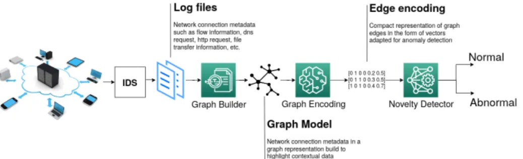
Sec2graph detects abnormal patterns in network traffic. Network event logs are used as an input for the whole process. The three key steps of sec2graph are presented in Figure 1.

Fig. 1: Overview of the sec2graph workflow

Section 2.1 explains how we build a graph of security objects from the network events; Section 2.2 explains how we encode this graph into vectors able to be handled by an auto-encoder; Section 2.3 explains how anomalies can be detected by the auto-encoder.

2.1 Building Security Object Graphs from Network Events

In this section, we formally define the graphs we introduce in this paper, and explain how we build them from logs.

A log file can be described as a sequence of n ordered events {e1, e2, ..., en}

where ei is an event resulting from the observation of activity in the network.

Each event is made of several fields that differ depending on the semantic of the event itself. Some of these fields are particularly relevant to identify links between events. For each type of event, we identify the most relevant fields to create one or several Security Objects (SOs). A SO is thus a set of attributes, each attribute corresponding to a particular event field.

For example, a network connection leads to four SOs: a source IP Address SO, a destination IP Address SO, a Destination Port SO and a last SO, the NetworkConnection itself that regroups attributes corresponding to the fields we identified as less important to create relations between events. For in-stance, the payload size attribute is captured as a mere attribute of the Network Connection object since there is no reason to believe that two events, having the same payload size, are linked. By contrast, two events for which the same IP addresses appear can be linked with high probability.

For each type of event, we designed a translation into a set of SOs. To keep track of each type of events, links are created between security objects that

represent this type. The different type of events considered are network connec-tion, application events (e.g., dns, dhcp, dce/rpc, ftp, http, kerberos, ssh, snmp, smtp,etc.), and information about transferred files and x509 certificates. All of these events are important in the context of intrusion detection because they may contain evidence of compromise. For example, network connection events indicate which devices are communicating and how. This can be useful for de-tecting port scans, or communications that violate internal security policies. Application events allow the capture of protocol-specific characteristics such as the versions used, thus revealing vulnerabilities. Finally, information about file transfers can be useful as they are a common way to spread viruses, for example by sending executable files.

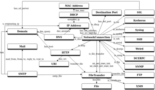
Fig. 2: Complete Security Objects and Relations Model Representation The graph model in Figure 2 shows the different types of SOs (nodes of the graphs) and their semantic links (edges of the graphs). For clarity reason, we have not represented the attributes of the SOs on this figure. Our model is suited to the pieces of information that are representative of network events. It can also evolve easily according to the needs of the analysts. For instance, the X509 object which corresponds to the certificate used during an SSL/TLS session was integrated in a second phase in accordance with the evolution of network communications that are increasingly encrypted.

More formally, our graphs are directed graphs G = (SO, E) with SO being the set of nodes and E being the set of edges. Let l ∈ E be a link between two nodes a and b. l is defined by the triple (a, b, ltype). ltypecorresponds to the type

of the link. For example, for a network connection event, a NetworkConnection SO is created and linked to an IPAddress SO: this link is of type has src address.

Figure 2 shows the different types of links between SOs. The semantic of these links is derived from the CybOX model [8].

To build the graph, we take as an input a set of network events coming from various log files. From each event, and according to it type, we extract the SOs and the links between them. In other words, we first build a sub-graph representing this event. We then take each SO of the sub-graph. If this SO already exists in the global graph (for instance, a same IPAddress was already identified in a previous event), we replace the SO in the new sub-graph by the SO that already exists in the global graph. Therefore, if an event contains an SO that was already found in a previous event, the sub-graph that represents it will be linked to the graph through this SO.

As an example, let’s consider three log events extracted from the Zeek [24] analysis of the CICIDS2017 dataset [31]. The three log events represent the same FTP connection analyzes by different modules of the Intrusion Detection System. The first event e1 is a report on the TCP network connection from the

IP address 192.168.10.15 to the IP address 192.168.10.50 on port 21. The second event e2gives the details of the FTP reply. The third event e3corresponds

to file transfer details. A graph for each of these three events is represented on the left hand of Figure 3. We represent the global graph composed of six SOs and obtained from the three previously described sub-graphs on the right hand of the figure: the first event is colored in blue surrounded by a solid line (e1), the second is in red surrounded by a dotted line (e2) and the third is in yellow surrounded by a small dotted line (e3). e1 and e2 shares a reference to the

same NetworkConnection SO (same uid value) and e2 and e3 share the same

FileTransfer SO (same fuid value). By combining the different log files, the graph makes possible to deduce relationships within different log events and thus to learn more complex patterns.

Fig. 3: (left) Building of sub-graphs from three events, (right) Complete graph issued from three events

2.2 Encoding the graph for machine learning

The second step of sec2graph transforms the graph we computed in a structure that can be processed efficiently by a machine learning algorithm. To the best of our knowledge, there does not exist a method to encode multi-attributes and heterogeneous graphs that would be considered as generically efficient. For example, an adjacency matrix is inefficient for large graphs. It also carries no information on nodes and edges. In our case, the encoding method must encode both the structure of the graph (i.e., the relations between the nodes) and the specific information associated with the nodes and the edges. Moreover, the result of the encoding should be of reasonable size while it should contain enough information to detect anomalies. Since there does not exist a single best method to encode our graph, we had to design one tailored to our specific case. ion on a new port. When a collection of similar data instances behave anomalously with respect to the entire dataset, the group of data instances is considered as a collective anomaly. For example, a deny of service can be considered as a collective anomaly. Contextual anomalies or conditional anomalies, are events considered as anomalous depending on the context in which they are found, for example, specific attack on vulnerable version of services or vulnerable network device.

We are looking for anomalies. A given SO can be linked to several events, normal or abnormal. An edge, on the other hand, is only related to the event that led to its construction. Therefore, the anomaly is not carried by the node (an IP address or a port are not abnormal per se) but by the edges that link the SOs together. Consequently, we have chosen to encode our graph by encoding each of its edges. To preserve the context of the event related to this edge, we have chosen the following pieces of information to encode an edge: the type of the edge, information about the source node and the destination node, information about the neighborhood of the source node and information about the neighborhood of the destination node. It should be mentioned that, by construction, a security event cannot be represented by a sub-graph with a diameter greater than three. Indeed, the translation method that we defined to convert events to sub-graph never produces a sub-graph that has a path between two nodes made of more than three edges.

In our graph, there are different kinds of attributes with categorical (ver-sion numbers, protocol types, etc.) or continuous (essentially size or duration) values. Anomaly detection requires to encode these two types of attributes in a unified way (see section 2.3). Therefore, categories must be determined for each attribute, even for continuous ones.

Determining categories. For each categorical attribute, we count the num-ber of occurrences of each category, for example, the numnum-ber of times the value ’tcp’ appears for the attribute ’protocol’. For single-value attributes such as port value, the number of occurrences is by construction always equal to one, since we create only one Port SO for this port number. In this type of cases, single-value attributes are distinguished by counting the number of edges of the

node carrying this single value attribute. In both cases, we sort them in descend-ing order and keep the N most represented categories that account cumulatively for 90% of the total number of occurrences or number of edges. If more than 20 categories remain, we only keep the 20 most represented categories. It should be noted that we choose the value 20 according to an analysis we performed on the CICIDS2017 dataset [31] that showed that considering more than 20 categories for an attribute does not improve detection.

To translate continuous attributes into categories, considering intervals (e.g. [0:10[, [10:20[, etc.) is not an option because this would not take into account the statistical distribution of values and would not be useful for the auto-encoder. Therefore, we categorize the continuous data according to the distribution of the attribute values since our data samples do not necessarily follow a usual probability law, but a law whose density function is a mixed density. To do that, we use the classical Gaussian Mixture Model (GMM), assuming that the values of the attributes follow a mixture of a finite number of Gaussian distributions. It has been shown that GMM gives a good approximation of densities [15]. Furthermore, this technique has already been used for anomaly detection [7].

Two methods exist to infer the Gaussian equation and classify the data. The first one, the expectation-maximization algorithm (EM), is the fastest algorithm for learning mixture models but it requires to define the number of Gaussian components to infer [10]. The second one uses the variational inference algo-rithm [5]. It does not require to define the number of components but it requires hyperparameters that might need experimental tuning via cross-validation. We choose the first technique to control the number of Gaussian and hence control the number of dimensions of our vector as we will associate one dimension to one component. The number of Gaussian distributions is determined by the classi-cal Bayes Information Criterion (BIC). This consists of successively classi-calculating mixtures of Gaussian in increasing numbers and choose the one with the lowest BIC. In practice, we do not mix more than eight Gaussian, because we found in our data set that the BIC is never smaller. The result is a mixture of no more than eight Gaussian, which brings us down to a case with no more than eight categories.

Encoding attributes using categories. Once we have determined all the categories for our dataset, we can encode the nodes as a binary vector. We proceed as follows.

To fit the auto-encoder, all entries need to be the same size. For each node and each attribute, we distinguish three cases: either the node has the attribute and its value corresponds to one of the categories of the attribute, or the node has the attribute but its value does not correspond to one of the categories, or the node does not have the attribute given its type (for instance, it is an IPAddress node and therefore does not have the port value attribute). The one-hot-encoding technique is used. For each node of the graph, we build a binary vector x of size N + 1, N corresponding to the number of categories. Each bit of this vector corresponds to a given category and is thus set to one if the attribute value of the

nodes is of this category. It is set to zero otherwise. One last bit with the value 0 is added to this vector to represent the category “other”. In the second case, each bit is assigned the value 0 and one last bit is added to ’1’ for the “other” category. Finally, in the last case, i.e., if the encoded attributes are not related to the type of the node, all the bits are assigned the value 0. This method makes it possible to encode uniformly all the nodes whatever there type. We build a vector for each attribute then we concatenate all these vectors into a binary vector corresponding to the encoding of our node.

Encoding the structure of the graph. The encoding of the attributes pre-sented above is relative to the information contained in the nodes’ attributes. Our representation also takes into account the structure of the graph and the types of the edges. To this end, we encode an edge as a vector resulting of the concatenation of information on (a) the type of this edge, (b) the attributes of its source node, (c) the attributes of its destination node, (d) information about the neighborhood of its source node and (e) information about the neighborhood of its destination:

– (a): there are 18 types of edges. For each edge, we encode its type using the same one-hot encoding technique that we use to encode the node’s attributes. – (b) and (c): We encode the attributes of the source node and destination

node as previously described.

– (d) and (e): for each source node and destination node, we select randomly 10.000 neighbors and compute the mean of their encoding vector. We choose 10.000 nodes because this allows us to reduce the computational complexity and we have determined that the mean does not change significantly above this threshold.

Considering that a l edge between s and d is of type ltype, as well as that the

s node has N (s) neighbors and the d node has N (d) neighbors, we randomly select 10,000 nodes in N (s) and N (d) to constitute a representative sample of the neighborhood N (s)sample and N (d)sample. It should be noted that we already

have the encoding of each of these nodes in the form of a binary vector each having the same size.

We define mean(−→encN (s)sample) and mean(−→encN (d)sample) as the bit-wise

aver-age of the vectors encoding each node of N (s)sampleand N (d)samplerespectively.

It should be noted that, at this point, the vector is made of continuous values between 1 and 0 for the encoding of the neighbors. We thus obtain a compact representation of the neighborhood of the node that is sufficient for the pro-cessing of the graph and to detect anomalies. In this compact representation, each element of each vector takes a value between 0 and 1, but each element corresponds to a category of a certain attribute. Therefore, this vector of val-ues between 0 and 1 gives an idea of the distribution of the categories in the considered neighborhood.

2.3 Novelty Detection with an Auto-encoder

We use an auto-encoder for novelty detection as already proposed by [2, 4, 6, 22, 29] in the security field where novelty is viewed as an anomaly that may be generated by an attack. An auto-encoder [19] learns a representation (encoding) of a set of pieces of data, typically for dimensional reduction. To do so, it learns a function that sets the outputs of the network to be equal to its inputs. It is made of two parts : an encoder and a decoder. The encoder compresses the input data into a low-dimensional representation, and the decoder generates a representation that is as close as possible to its original input from the reduced encoding.

The inputs to our auto-encoder consist of the vectors whose construction was explained in section 2.2. Recall that these vectors encode the following informa-tion: edge type, source node attributes, destination node attributes, source node neighborhood attributes, and destination node neighborhood attributes. The first three pieces of information are encoded by binary vectors while the last two are encoded by vectors whose components are continuous values between 0 and 1 (see 2.2). In a similar case, Bastos et al. [9] showed that it was desirable to have a single encoding function (which makes it possible to take into account possible correlations between the different types of encoding) and a decoding function specific to each type of information (binary vs. between 0 and 1) or specific to each piece of information.

Our auto-encoder, therefore, has five outputs and uses two types of loss functions: binary cross-entropy, that is suited to binary values, and mean-square error, that is suited to continuous values. The result is made of five error values between 0 and 1. To determine whether there is an anomaly, we calculate an overall error which is the sum of these five errors and raise an anomaly alert if it reaches a certain threshold. This threshold is set experimentally (see 3.2). Of course, the lower it is, the more alerts we have and the greater the risk of false positives. The analyst sets the threshold value according to his or her monitoring context by lowering the value if it is more important for the analyst not to miss any attacks than to have a large number of false positives.

3

Implementation and experimental results

This section details our implementation choices, experiments, and analysis. We first describe the technologies used, the dataset and the evaluation criteria in Section 3.1. We then carefully choose a threshold value in Section 3.2. Finally, we dive into the results obtained by deploying the sec2graph approach compared to other approaches based on anomaly detection in Section 3.3.

3.1 Experimental setup

Dataset. We choose to use the CICIDS2017 dataset [31] that is made of five pcap and csv files encompassing more than two million network sessions. This

dataset was generated at the Canadian Cybersecurity Institute at the University of New Brunswick and contains five days (Monday to Friday) of mixed traffic, benign and attacks such as DoS, DDoS, BruteForce, XSS, SQL injection, infil-tration, port scan, and botnet activities.

Normal traffic was generated using the CIC-B-Profile [31] system, that can reproduce the behavior of 25 users using various protocols (FTP, SSH, HTTP, HTTPS and SMTP). Attacks were executed using classic tools such as Metas-ploit and Nmap. This dataset is labeled, i.e., we know when attacks occur and when the traffic is normal. For example, the traffic captured on Monday is en-tirely normal. According to [13], the CICIDS2017 dataset is the most recent one that models a complete network configuration with components such as firewalls, routers, modems, and a variety of operating systems such as Windows, Ubuntu Linux or Macintosh and that has been used in several studies. The protocols in the capture (e.g., HTTP, HTTPS, FTP, SSH) are representative of protocols used in a real network and a variety of common attacks are covered. The data set is also labeled, allowing us to quantify the effectiveness of our method. To generate log files from the capture files, we used the Zeek IDS tool (formerly Bro) that can generate network and application logs such as connections, http communications or file transfers. The default configuration for the Zeek IDS was applied.

Implementation details and configuration. We chose the Python language and we use a Gremlin API [28] for the construction of the graph from the events logs and the manipulation of this graph. Indeed, the gremlin language is partic-ularly well adapted to the construction and manipulation of graphs. Besides, we used the Python language for the implementation of the auto-encoder based on the Keras library.

We used a Janusgraph database with an external index backend, Elastic-search, and a Cassandra storage backend to store the graph data. We choose these technologies for scalability as they are adapted to large graph databases. Experiments were performed on a Debian 9 machine with 64 GB RAM.

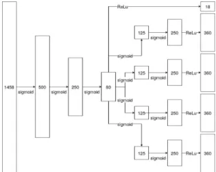
The structure of our auto-encoder is depicted in Figure 4. The sizes of both the input layer and the output layers (18+4*360=1458 neurons) come from the sizes of our vectors (recall that the output should be equal to the output). The auto-encoder counts five hidden layers: the diversity of the SOs in the graph leads to very diverse encoding and thus this number of hidden layers is suited for learning complex relations between the different bits of the vectors. The intermediate layer between the encoder and the decoder has a size of 80: the input vectors are indeed sparse, thus we choose a little number of neurons for this layer. The number of neurons in each layer and the number of hidden layers was determined by experimentation, trying different values looking for a minimum value for the reconstruction error. We choose a number of epochs (the number of iteration of the forward and backpropagation phase) of 20 as experiments show that the reconstruction error did not decrease significantly for a larger number of epochs. We choose the Adam optimizer with a learning rate of 0.001 to

back-Fig. 4: Structure of the auto-encoder

propagate the reconstruction error as it is well-adapted when more than one hidden layer is used.

To train our auto-encoder, we used during a first phase (learning phase), the data captured on Monday as it is entirely normal. This data is split in a training set and a validation set with a validation split of 0.1. This allows to validate the model on unseen data and thus prevent overfitting. Depending on the various parameters we have, the learning phases took about an hour. In the second phase (anomaly detection phase), we used the whole dataset (Monday to Friday) to evaluate the detection capacity of our approach.

Evaluation criteria. Our approach seeks to identify anomalies related to links between objects. Classical approaches seek to identify anomalies relating to events. Although our ultimate goal remains to present the anomalous edges to the analyst, in this section, to compare ourselves to the classical approaches, we determine from the anomalous edges we find in the graph the events that gave birth to them. We consider as abnormal any event whose representation contains at least one abnormal edge.

All the results presented in this section are related to events. These are processed in one-hour shifts. For each time slot, we build a graph, then the vectors to enter into the auto-encoder and finally we evaluate the novelty of each vector.

In addition to the number of true positives (TP), false positives (FP), true negatives (TN) and false negatives (FN), we evaluate our results through the fol-lowing standard metrics: Precision, Recall, F1-score, False Positive Rate (FPR) and Accuracy. The Precision gives the ratio of real anomalous events among all the events declared as anomalous. The Recall gives the proportion of events correctly detected as anomalous among all the really anomalous events. The F1-Score is the harmonic mean of the Precision and Recall. The FPR is the proportion of events for which an anomaly has wrongly been emitted and the

accuracy is the number of events correctly classified (as anomaly or as normal events) divided by the total number of events. Formally, these criteria can be defined as follows: P recision = T P T P + F P; Recall = T P T P + F N; F P R = F P F P + T N; Accuracy = T P + T N T P + F N + T N + F P; F 1score = 2 ∗ P recision ∗ Recall P recision + Recall 3.2 Defining an optimal threshold for detection

In this section, we present the experiments conducted to determine the threshold value to be used. As noted above, the analyst sets this threshold value according to his or her supervisory context, lowering the threshold value if it is more important for the analyst not to miss any attacks than to have to eliminate a large number of false positives.

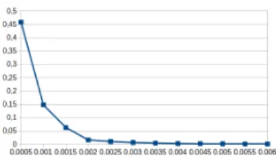
We determine the value of the threshold as follows: first, we consider all the events of Monday, a day without attacks. With this data, we determine the rate of false positives according to the detection threshold. We obviously want the lowest possible false-positive rate. The curve in Figure 5 shows the evolution of the FPR as a function of the detection threshold. A threshold of 0.003 gives us an FPR of 0.031. In the figure, for threshold values on the right of the value of 0.003, the FPR decreases weakly, while for threshold values on the left, it strongly increases.

Fig. 5: False Positive Rate (FPR) according to the value of the detection thresh-old on Monday data (normal events).

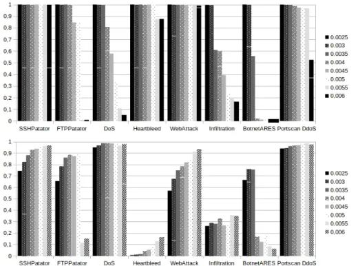
We conclude that a threshold higher than 0.003 should be retained. To deter-mine the value of this threshold more precisely, we need to consider the different types of attacks in our dataset and determine the value that allows the most efficient detection of these attacks. For this purpose, we consider the time slots during which each attack occurs. For example, the FTP Patator attack takes place on Tuesday from 9:20 to 10:20, so we consider the data between 9:00 and 11:00. During these time slots in which the attacks take place, we want the max-imum number of events belonging to the attacks to be detected as anomalies while keeping the number of false positives as low as possible. In other words, we naturally want to maximize precision and recall. Figure 6 gives the values of recall and precision as a function of the detection threshold for the different types

of attacks in the CICIDS2017 dataset. We varied this threshold over the entire range for which this variation has a significant impact on recall and precision.

Fig. 6: Values of Recall (top figure) and Precision (bottom figure) for the range of variation of the threshold leading to a significant evolution of these values.

On the diagram at the top of the figure, it can be seen that a quasi-optimal recall can be obtained (between 0.993 and 1) for a threshold value of 0.003. On the diagram of the bottom of the figure, we also see that for this threshold value, the precision is between 0.675 and 0.967, except for the Heartbleed attack (0.012) and the infiltration attack (0.287). However, increasing the threshold further does not significantly increase the precision, but does significantly decrease the recall for infiltration and botnet. We, therefore, conclude that we can retain a threshold value of 0.003.

The two cases of low precision, i.e., Heartbleed and infiltration can be ex-plained differently. In the case of Heartbleed, the low precision is exex-plained by the silent nature of this attack. Indeed, if we detect 100% of the events related to the attack for a threshold of 0.003, this represents only eight network connec-tions compared to almost 93.000 network connecconnec-tions that took place during the attack. While the FPR is consistent with other slots in our dataset, the 93.000 normal network connections lead to 681 false positives and thus decrease the precision. In the case of the infiltration attack, the low accuracy is explained by

an abnormally large number of false positives. The infiltration attack is indeed followed by a portscan performed by the victim of the infiltration. The pertur-bation being massive, it impacts the neighborhood of the events linked to the scan. This leads to considering a large amount of this neighborhood abnormal, even for normal events, leading to a high rate of false positive.

3.3 Comparison with other anomaly detection algorithms on the same dataset

To compare our results with the state of the art, we have taken the results of three studies on attack detection that use the same dataset as we do, the CICIDS2017 dataset 5_{. These studies are the only three that present results according to all}

or part of the criteria we have defined above and the comparison is therefore possible.

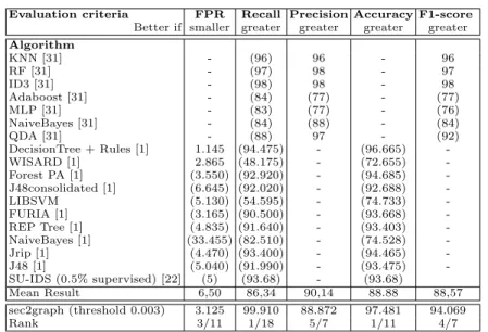
Evaluation criteria FPR Recall Precision Accuracy F1-score Better if smaller greater greater greater greater Algorithm KNN [31] - (96) 96 - 96 RF [31] - (97) 98 - 97 ID3 [31] - (98) 98 - 98 Adaboost [31] - (84) (77) - (77) MLP [31] - (83) (77) - (76) NaiveBayes [31] - (84) (88) - (84) QDA [31] - (88) 97 - (92) DecisionTree + Rules [1] 1.145 (94.475) - (96.665) -WISARD [1] 2.865 (48.175) - (72.655) -Forest PA [1] (3.550) (92.920) - (94.685) -J48consolidated [1] (6.645) (92.020) - (92.688) -LIBSVM (5.130) (54.595) - (74.733) -FURIA [1] (3.165) (90.500) - (93.668) -REP Tree [1] (4.835) (91.640) - (93.403) -NaiveBayes [1] (33.455) (82.510) - (74.528) -Jrip [1] (4.470) (93.400) - (94.465) -J48 [1] (5.040) (91.990) - (93.475) -SU-IDS (0.5% supervised) [22] (5) (93.68) - (93.68) Mean Result 6,50 86,34 90,14 88.88 88,57 sec2graph (threshold 0.003) 3.125 99.910 88.872 97.481 94.069 Rank 3/11 1/18 5/7 1/11 4/7

Table 1: Comparison of False Positive Rate (FPR), Recall, Precision, Accuracy, and F1-score results (in %) for supervised and semi-supervised approaches of literature and sec2graph. The values in brackets are worse than those obtained with sec2graph. The rank indicates the ranking of sec2graph in relation to other approaches.

Sharafaldin et al. [31] compares the results of seven supervised classical ma-chine learning algorithms applied on this dataset: K-Nearest Neighbors (KNN),

5

Another study was published very recently [11] that deals with the 2018 version of the CICIDS data. These data are richer in terms of protocols but different in terms of attacks. While we cannot compare our proposal to this study, we have a work in progress in this direction.

Random Forest (RF), ID3, Adaboost, Multilayer perceptron (MLP), Naive-Bayes (NB) and Quadratic Discriminant Analysis (QDA), that are all super-vised machine learning algorithms. Ahmim et al. [1] compare the results of twelve classical or more recent classification algorithms: DecisionTree and rules, WISARD, Forest PA, J48 consolidated, LibSVM, FURIA, REP Tree, Naive-Bayes, Jrip, J48, MLP, and RandomForest. Since the latter two algorithms were used in both studies, only the best results were retained in the comparison. Min et al. [22] propose a semi-supervised method SU-IDS based on an auto-encoder and a classification method. The SU-IDS experiments were carried out with a variable number (from 0.5% to 100%) of labeled data. To compare our proposal to a method close to an unsupervised model, we have chosen to use the results of the tests carried out on a sample with 0.1% of labeled data.

All these algorithms were tested starting from a dataset containing 80 fea-tures selected according to their relevance for the detection of attacks using the CICFlowMeter tool [31]. In the case of the first seven algorithms listed above, the authors trained their algorithms on a specifically chosen subset of the 80 attributes using a Random Forest Regressor. These attributes were chosen be-cause they were most likely to help detect the attacks in the dataset and thus improved the performance of the algorithms for these specific types of attacks. In our case, we used all the features contained in Zeek event logs without making a prior selection according to their relevance for observing attacks. Our objective is to measure the ability of the auto-encoder to choose the most relevant features to represent a normal behavior in our dataset without targeting specific types of attack.

Table 1 provides a comparison of the classical learning machine algorithms listed above against our approach sec2graph with the optimal value previously determined for the detection threshold. Results of the different algorithms come directly from the original papers and parameters of the algorithms can be as-sumed to have been optimized to produce the best possible results.

The values in this table show that, although being an unsupervised approach, sec2graph achieves performances at worst slightly below the average of those obtained by the supervised approaches it is compared to. Given the strategy we have adopted to set the detection threshold, we achieve the best performance in terms of recall, with 99.91% of attack events correctly marked as abnormal (all attacks tested generate marked events). Nevertheless, sec2graph’s ranking remains close to the average in terms of precision, which means that the analyst will not be drowned by false positives: 88.872% of alerts are indeed true positives. Moreover, we did not select attributes according to the type of attacks we want to detect, allowing us to adapt to new kinds of attacks.

4

Discussion

While CICIDS2017 is arguably one of the most realistic and reasonably large datasets, it contains numerous attacks that impact the total volume of network communications. We trained our model only with the normal traffic on Monday

because the dataset on other days contains far too many attack sessions. While the hypothesis of a learning dataset without attacks is strong, it is realistic to think that attacks can be very limited in some real-life network traffic samples. Auto-encoders also learn a general model, not taking into account particular cases such as these attacks. Future work on a learning dataset with a low attack proportion would allow to validate this hypothesis.

As discussed in section 3.2, some attacks such as Infiltration are well detected but also induce many false positives. Indeed, in this very case, nodes identified as abnormal impact the calculation on their normal neighboring nodes, making them look abnormal. Refining the method to calculate the reconstruction error could reduce this effect. More generally, incorrectly labelling 3% of all the events as abnormal (see FPR in table 1 is way too high. However, the graph approach allows the analyst to take into account a large number of events at once. More-over, the use of an auto-encoder allows a better interpretation of the results. During our analysis, we defined a reconstruction error corresponding to the sum of the reconstruction errors, but it is possible to obtain the detail of the values expected by the model and thus better interpret the results.

We tested our algorithm on data where normal traffic does not evolve while in a real environment network activities, devices and behaviors change over time. Since auto-encoders allow for iterative learning, it is possible to use new data to evolve the model and learn new behaviors. This can be used to eliminate recurring false positives or to track the evolution of network activities.

To cope with new type of data or new networks, changing the number of layers and neurons of the auto-encoder is needed. Thus, we cannot directly transfer the learning result to a new context. However, study of the FPR (see section 3.2) allows to adjust the parameters and choose a threshold for reconstruction error. Diverse network communications and complexity require a larger number of neurons for learning while a simple network on which actions are not very diversified requires to decrease the number of neurons to avoid overfitting.

5

Related work

In this section, we position our work in relation to similar approaches in the lit-erature. To our best knowledge, at the time of writing, none of these approaches has sought to detect anomalies on graphs using auto-encoders. Here, we position our work, firstly with respect to pieces of work that relied on graphs for anomaly detection, and secondly with respect to pieces of work that used auto-encoders for anomaly detection.

5.1 Using graph structures for anomaly detection

In the field of intrusion anomaly, graph structures have often been used. Her-cule [25] represents inter-log similarities within a graph of log events. In this representation, a node represents a log event and an edge represents a prede-fined similarity relationship between two logs events. Clustering techniques are

then applied to the graph to identify the set of events related to a given attack. Strictly speaking, there is no anomaly detection but the identification of infor-mation related to a known attack occurrence identified thanks to a compromise indicator. Experiments on APT attacks shows that the system performs well in this task (accuracy of 88% on average), and once the events related to the attack have been identified, it allows forensic analysis of the attack.

Other work relates to forensic analysis and exploits graph structures. For example, King and Chen [16], as well as Goel et al. [14], propose to reconstruct a chain of events in a dependency graph to explain an attack. In [21], Milajerdi et al. use audit logs to reconstruct the history of attacks using traces from common Advanced Persistent Threat (APT) attacks. Kobayashi et al. [17] use syslog events to infer causality between security system events. These proposals are however limited since they only consider one type of event format. Xu et al. [32] represent, as a graph, the causal dependency among system events.

Other works use graphs to detect attacks and more precisely to detect bot-nets [23, 12, 18]. They use network-related data to build topological graphs with nodes representing hosts and links representing network communication between them. They then use clustering, PageRank algorithm or statistical-based mining techniques on graphs to identify abnormal network traffic based. While having similar objective, we do not limit to botnet detection. Furthermore, in addition to the fact that we process our graphs with an auto-encoder for anomaly detec-tion, our dataset is richer since not limited to netflow data. This rich data also allows us to take into account the global context in which the attacks occur.

Finally, Log2vec [20] detects users malicious behavior based on a clustering algorithm applied to relations among users operations. Log2vec represents user’s actions with small graphs and embeds them in a vector by using a random-based walk algorithm. By contrast, we represent all network events in one big graph and detect anomalies that occur on multiple devices by multiple attackers. 5.2 Using auto-encoders for anomaly detection

Several pieces of work already used auto-encoders for anomaly detection [4, 6, 22, 2, 29], among which only [6, 29] proposes unsupervised approaches.

The authors of [6] use two types of auto-encoders namely, stochastic de-noising auto-encoder and deep auto-encoder, to detect anomaly in the NSL-KDD dataset. The experiments conducted by the authors show that their model achieves an F1-score score respectively of 89.5% and 89,3%, a recall of 87.9% and 83.1% and a precision of 91.2% and 96.5%. However, the dataset used con-tains redundant data that can distort the results obtained by learning machine algorithms. In our study, we used the CICIDS2017 dataset that addresses the problems posed by the NSL-KDD dataset and we were able to obtain better results thanks to our graph representation of SOs.

The authors of [22] propose to remedy the problems of data with little or no security label by proposing an unsupervised and semi-supervised approach. The idea is to use an auto-encoder in association with a classification algorithm for the semi-supervised approach. The latter is then trained on a restricted portion

of labeled data. In the unsupervised approach, the auto-encoder is used alone. The study was carried out on the NSL-KDD and CICIDS2017 datasets. The results are good only in the semi-supervised approach, even if the unsupervised approach seems to isolate some attacks. In our work, on the CICIDS2017 data and with an unsupervised approach, we obtain better detection results, especially for false positives. Our graph approach handles heterogeneous types of events and links between these events, allowing us to detect anomalies without using a supervised algorithm.

In [29], the authors propose to use an auto-encoder to detect intrusion on IoT radio networks. The approach is based on the monitoring of the communication activities generated by the connected objects. The radio-activities patterns are then encoded in features specific to the IoT domain and normal activities are then learned with the auto-encoder to detect anomalies in a second phase. Simi-larly, Kitsune [33] is an auto-encoder-based NIDS capable of extracting features and creating a dynamically unsupervised learning model that has been tested for IoT devices. These methods are specific to the considered context but proposes, as in our case, an unsupervised intrusion detection system to detect anomalies with the help of an auto-encoder.

The other studies mentioned at the beginning of this paragraph [4, 2] add a supervised layer to the unsupervised output of the auto-encoder. The gen-eral idea is to use the auto-encoder to identify normal traffic almost certainly. Traffic that is not considered normal by the auto-encoder is then provided to a supervised classification device, trained on data labeled to identify attacks. We differ from this work since we refuse to label data, contenting ourselves with learning attack-free data. Indeed, in a production environment, the data is much too voluminous to be possible to label them. Moreover, the experimental results obtained by these other studies are based on data that are different from ours. It is therefore difficult if not impossible to compare these experimental results with ours.

6

Conclusion and Future Work

We proposed in this paper a graph representation of security events that under-lines the relationship between them. We also proposed an unsupervised technique built on an auto-encoder to efficiently detect anomalies on this graph represen-tation. This approach can be applied to any data set without prior data labeling. Using the CICIDS2017 dataset, we have shown that the use of graph structures to represent security data coupled with an auto-encoder gives results that are as good as or better than the supervised machine learning methods.

We are currently conducting new experiments with a wider neighborhood in the encoding of the graph to evaluate the potential improvement of intrusion detection and reduction of the number of false positives. To further improve our detection results, we plan to use another kind of encoder (LSTM auto-encoder) to take temporal links between events into account in addition to logical links that we already take into account. As these improvements should lead to

an increased duration of this learning phase, we will investigate a reduction of the size of the encoding of the nodes by using entity embedding instead of one-hot encoding. Another area for improvement is related to the usability and interpretability of results by a security analyst. Here, the idea is to present to the analyst a graphical view of the detected anomalies, based on the SOs graphs that we have defined. We want to provide to the analyst the subsets of the edges of this graph that have been detected as abnormal, as well as of course the SOs linked by these edges. We believe that this would help the analyst eliminating false positives or reconstructing global attack scenarios.

References

1. Ahmim, A., Maglaras, L., Ferrag, M.A., Derdour, M., Janicke, H.: A novel hier-archical intrusion detection system based on decision tree and rules-based models. In: 15th International Conference on Distributed Computing in Sensor Systems (DCOSS) (2019)

2. Al-Qatf, M., Lasheng, Y., Al-Habib, M., Al-Sabahi, K.: Deep learning approach combining sparse autoencoder with SVM for network intrusion detection. IEEE Access (2018)

3. Anagnostopoulos, C.: Weakly supervised learning: How to engineer labels for ma-chine learning in cyber-security. Data Science for Cyber-Security (2018)

4. Andresini, G., Appice, A., Di Mauro, N., Loglisci, C., Malerba, D.: Exploiting the auto-encoder residual error for intrusion detection. In: IEEE European Symposium on Security and Privacy Workshops (EuroS&PW) (2019)

5. Attias, H.: A variational baysian framework for graphical models. In: Advances in neural information processing systems (2000)

6. Aygun, R.C., Yavuz, A.G.: Network anomaly detection with stochastically im-proved autoencoder based models. In: IEEE 4th International Conference on Cyber Security and Cloud Computing (CSCloud) (2017)

7. Bahrololum, M., Khaleghi, M.: Anomaly intrusion detection system using hier-archical gaussian mixture model. International journal of computer science and network security (2008)

8. Barnum, S., Martin, R., Worrell, B., Kirillov, I.: The cybox language specification. draft, The MITRE Corporation (2012)

9. Bastos, I.L., Melo, V.H., Gon¸calves, G.R., Schwartz, W.R.: Mora: A generative approach to extract spatiotemporal information applied to gesture recognition. In: 15th IEEE International Conference on Advanced Video and Signal Based Surveillance (AVSS) (2018)

10. Dempster, A.P., Laird, N.M., Rubin, D.B.: Maximum likelihood from incomplete data via the EM algorithm. Journal of the Royal Statistical Society: Series B (Methodological) (1977)

11. Ferrag, M.A., Maglaras, L., Moschoyiannis, S., Janicke, H.: Deep learning for cyber security intrusion detection: Approaches, datasets, and comparative study. Journal of Information Security and Applications (2020)

12. Fran¸cois, J., Wang, S., Engel, T., et al.: Bottrack: tracking botnets using netflow and pagerank. In: International Conference on Research in Networking (2011) 13. Gharib, A., Sharafaldin, I., Lashkari, A.H., Ghorbani, A.A.: An evaluation

frame-work for intrusion detection dataset. In: International Conference on Information Science and Security (ICISS) (2016)

14. Goel, A., Po, K., Farhadi, K., Li, Z., De Lara, E.: The taser intrusion recovery system. In: ACM SIGOPS Operating Systems Review (2005)

15. Goodfellow, I., Bengio, Y., Courville, A.: Deep learning. MIT press (2016) 16. King, S.T., Chen, P.M.: Backtracking intrusions. In: ACM SIGOPS Operating

Systems Review (2003)

17. Kobayashi, S., Otomo, K., Fukuda, K., Esaki, H.: Mining causality of network events in log data. IEEE Transactions on Network and Service Management (2017) 18. Lagraa, S., Fran¸cois, J., Lahmadi, A., Miner, M., Hammerschmidt, C., State, R.: Botgm: Unsupervised graph mining to detect botnets in traffic flows. In: 1st Cyber Security in Networking Conference (CSNet) (2017)

19. Le Cun, Y., Fogelman-Souli´e, F.: Mod`eles connexionnistes de l’apprentissage. In-tellectica (1987)

20. Liu, F., Wen, Y., Zhang, D., Jiang, X., Xing, X., Meng, D.: Log2vec: A het-erogeneous graph embedding based approach for detecting cyber threats within enterprise. In: Proceedings of the ACM SIGSAC Conference on Computer and Communications Security (2019)

21. Milajerdi, S.M., Gjomemo, R., Eshete, B., Sekar, R., Venkatakrishnan, V.: Holmes: real-time apt detection through correlation of suspicious information flows. In: IEEE Symposium on Security and Privacy (SP) (2019)

22. Min, E., Long, J., Liu, Q., Cui, J., Cai, Z., Ma, J.: SU-IDS: A semi-supervised and unsupervised framework for network intrusion detection. In: International Confer-ence on Cloud Computing and Security (2018)

23. Nagaraja, S., Mittal, P., Hong, C.Y., Caesar, M., Borisov, N.: Botgrep: Finding P2P bots with structured graph analysis. In: USENIX security symposium (2010) 24. Paxson, V.: Bro: a system for detecting network intruders in real-time. Computer

networks (1999)

25. Pei, K., Gu, Z., Saltaformaggio, B., Ma, S., Wang, F., Zhang, Z., Si, L., Zhang, X., Xu, D.: Hercule: Attack story reconstruction via community discovery on correlated log graph. In: Proceedings of the 32th Annual Conference on Computer Security Applications (2016)

26. Pimentel, M.A., Clifton, D.A., Clifton, L., Tarassenko, L.: A review of novelty detection. Signal Processing (2014)

27. Pincus, R.: Barnett, v., and lewis t.: Outliers in statistical data. j. wiley & sons 1994, xvii. 582 pp.,£ 49.95. Biometrical Journal (1995)

28. Rodriguez, M.A.: The gremlin graph traversal machine and language. In: Proceed-ings of the 15th Symposium on Database Programming Languages (2015) 29. Roux, J., Alata, E., Auriol, G., Kaˆaniche, M., Nicomette, V., Cayre, R.: Radiot:

Radio communications intrusion detection for iot-a protocol independent approach. In: IEEE 17th International Symposium on Network Computing and Applications (NCA) (2018)

30. Scarfone, K., Mell, P.: Guide to intrusion detection and prevention systems (IDPS). Tech. rep., National Institute of Standards and Technology (2012)

31. Sharafaldin, I., Lashkari, A.H., Ghorbani, A.A.: Toward generating a new intrusion detection dataset and intrusion traffic characterization. In: ICISSP (2018) 32. Xu, Z., Wu, Z., Li, Z., Jee, K., Rhee, J., Xiao, X., Xu, F., Wang, H., Jiang, G.:

High fidelity data reduction for big data security dependency analyses. In: ACM SIGSAC Conference on Computer and Communications Security (2016)

33. Yisroel, M., Tomer, D., Yuval, E., Asaf, S.: Kitsune: An ensemble of autoencoders for online network intrusion detection. In: Network and Distributed System Secu-rity Symposium (NDSS) (2018)