HAL Id: hal-01672868
https://hal.archives-ouvertes.fr/hal-01672868
Submitted on 13 Nov 2019
HAL is a multi-disciplinary open access
archive for the deposit and dissemination of
sci-entific research documents, whether they are
pub-lished or not. The documents may come from
teaching and research institutions in France or
abroad, or from public or private research centers.
L’archive ouverte pluridisciplinaire HAL, est
destinée au dépôt et à la diffusion de documents
scientifiques de niveau recherche, publiés ou non,
émanant des établissements d’enseignement et de
recherche français ou étrangers, des laboratoires
publics ou privés.
Efficient and large-scale land cover classification using
multiscale image analysis
François Merciol, Thibaud Balem, Sébastien Lefèvre
To cite this version:
François Merciol, Thibaud Balem, Sébastien Lefèvre. Efficient and large-scale land cover classification
using multiscale image analysis. Big Data from Space, 2017, Toulouse, France. �hal-01672868�
EFFICIENT AND LARGE-SCALE LAND COVER CLASSIFICATION USING MULTISCALE
IMAGE ANALYSIS
Franc¸ois Merciol, Thibaud Balem and S´ebastien Lef`evre
Universit´e Bretagne Sud – IRISA
Campus de Tohannic, BP 573, 56017 Vannes Cedex, France
ABSTRACT
While popular solutions exist for land cover mapping, they become intractable when in a large-scale context (e.g. VHR mapping at the European scale). In this paper, we consider a popular classification scheme, namely combination of Differential Attribute Profiles and Random Forest. We then introduce new developments and optimiza-tions to make it: i) computationally efficient; ii) memory efficient ; iii) accurate at a very large scale; and given its efficiency, iv) able to cope with strong differences in the observed landscapes through fast retraining. We illustrate the relevance of our proposal by reporting computing time obtained on a VHR image.
Index Terms— Big Data, Differential Attribute Profiles, Max-Tree, Land Cover Mapping, Large-Scale Classification
1. INTRODUCTION
With the proliferation of Earth Observation sensors, as well as their continuously increasing performances (spatial resolution, revisit time, etc.), remote sensing has entered in the Big Data era. While in this context, dedicated architectures (clouds, HPC) represent a major component and various experiments have been reported, there is still an effort to be made on the algorithms themselves to make them adapted to large-scale, data- and computationally-intensive challenges raised, such as sub-metric land cover mapping at a con-tinental scale, as provided in some Copernicus products. Indeed, Europe with its area of 10 millions of sq.km corresponds to a map of 40 TeraPixels at 50cm (Pleiades resolution) or 100 TeraPixels at 31cm (WorldView-3 resolution).
In the context of land cover mapping, the standard approach is to first characterize each single pixel by some features extracted from the original image, and then apply a supervised classification tech-nique. While various options exists for these two steps, we can still observe some trends in the remote sensing community. As far as fea-ture extraction is concerned, beyond spectral information, multiscale spatial analysis has shown a strong ability to offer a discriminating characterization of various land use/land cover classes, with for in-stance the popular Differential Attribute Profile [1] and its many re-cent extensions (e.g., [2]). Supervised classification, where a model is first trained based on some reference data before been able to pre-dict the class of a new pixel, has been achieved with many methods in remote sensing, the two most popular being Support Vector Machine (SVM) and Random Forest (RF). The latter has the ability to eval-uate the relevance of the different dimensions of the feature space and their influence on the classification process. Besides, as a deci-sion tree, it helps the understanding of the classification rules that are
The authors acknowledge the support of the French Agence Nationale de la Recherche (ANR) under reference ANR-13-JS02-0005-01 (Asterix project); and SIRS for providing the use case, data, and funding.
used. It is thus a solution commonly adopted in remote sensing [3]. Furthermore, when combined with DAP, RF usually achieves better results. Thus, in the sequel of this paper, we will use such a com-bination “DAP+RF” as a baseline. For the sake of research repro-ducibility, we rely here solely on open-source solutions. RF imple-mentation is provided by the Shark library1, while DAP relies on our
own implementation in the Triskele library2acting as a new remote module for the OTB framework3. Nevertheless, a significant gain in terms of classification accuracy has been achieved with deep learn-ing [4, 5], and thus deep architectures are gainlearn-ing increaslearn-ing interest. However, these solutions still require a high computational cost and a heavy training process, and thus cannot be considered as a relevant solution for large-scale mapping yet.
We propose here an overall process that fits the large-scale re-quirements, minimizing the computational cost as well as the mem-ory footprint. Furthermore, thanks to this efficiency, we are able to retrain a classifier for each novel scene to be analyzed, leading then to a straightforward approach to ensure robustness to the high variability of the land cover classes observed in the various acquired scenes. Beyond the overall process, we specifically focus on the fea-ture extraction step for which we introduce a novel algorithm for efficient (both in time and space) tree construction that improves our former findings [6]. We also extend previous work on computing DAP on derived features such as NDVI [7], and demonstrate here the relevance of computing DAP on textural features.
2. OVERALL WORKFLOW
As already stated, large-scale classification brings three complemen-tary issues that are tackled in this paper: i) computational complex-ity that is addressed through efficient algorithms and reduction of the data to be processed at the different steps; ii) memory cost that is addressed through optimizations allowing to limiting the mem-ory footprint of the overall process; and iii) variability of the land cover class (e.g. spectral signature of the forest might differ between Mediterranean area and Scandinavia). In order to address these chal-lenges, we rely solely on method efficiency. More precisely, we do not consider domain adaptation techniques to adapt the classification model to each novel scene to be mapped. We rather assume that, given a near real time overall process, a user is able to provide some samples, train a classification model from these samples, predict the labels for the unlabeled pixels, visually or quantitatively assess the accuracy of the produced map, and update the samples (and then the model) until the obtained accuracy is satisfying. Let us note that this process actually fits many operational contexts, where the accuracy
1http://image.diku.dk/shark
2https://sourcesup.renater.fr/triskele 3https://www.orfeo-toolbox.org
requirements impose some manual assessment/correction as a post-processing step. Our workflow is given in Fig. 1 and applied for each new scene to be mapped. To ensure efficiency in a large-scale context, parallelism is mandatory and has been made explicit.
1. add to the original image some additional bands (e.g., NDVI, texture, etc.); each novel band is built in parallel; 2. compute a min- and/or a max-tree per band; subtrees are built in parallel for each tile, and then merged together; for the sake of parallelism, the tiles contain a similar amount of pixels, but there is no restriction regarding their specific shape (see Sec. 3);
3. provide reference samples from existing maps, ground truth data, or visual analysis;
4. characterize samples, based on the two following steps: (a) characterize each node by some attributes (e.g., area, standard deviation, moment of inertia, etc.); with attributes being incrementally computed from leaves to root, the parallelism occurs over nodes within each tree level;
(b) filter the tree and produce the full DAP feature vector; each feature vector (related to a unique pixel) is computed in parallel;
5. train the classifier on all features and evaluate it; 6. add new samples (step 3), characterize them (step 4)
and update the model (step 5) as long as it is necessary; select the subset of relevant features for classification; 7. using the selected set of features, perform land cover
mapping, i.e.:
(a) characterize all pixels;
(b) predict the classes using the trained model; 8. achieve a manual post-processing.
Fig. 1. Overall workflow
Classification is achieved with Random Forest (RF). Since RF is able to identify the important features in a classification process, we apply it on the full set of DAP features but only to the samples in steps 4 and 5; while in steps 7 (a) and (b), we consider all pixels but only a subset of the features. This actually leads to significant reduction of both computational and memory costs.
Feature extraction is performed with Attribute Profiles (AP), obtained by applying filters with increasing level on an input image, and efficiently computed from tree-based image representations. The original AP can be replaced by its differential version where differences between the filtered images form the feature vectors. Furthermore, instead of using the original image band, it has been shown recently that AP (or DAP) can be computed on derived fea-tures such as NDVI [7]. We follow this approach here and we propose to compute DAP over original bands, NDVI, as well as some additional bands bringing texture information. More precisely, we consider the L1 norm of the image gradient computed with the
Sobel masks. While there exists other popular texture descriptors (such as Haralick features), our choice has been motivated by the very low computational cost of Sobel gradient (i.e. each pixel is only
read 4 times). Let us note that the texture can then be computed over any of the input bands, including also the NDVI band. Computing DAP on Sobel information offers an efficient way to characterize the behavior of the edge information at multiple sizes.
3. TREE CONSTRUCTION
Our proposal assumes that the image features can be extracted very efficiently. The tree construction step is thus a key step in the pro-cess. In our previous work [6], we have introduced a novel algorithm for tree construction. We have however observed that, while the al-gorithm was intrinsically multi-threaded, the merging step might be particularly costly at the lowest levels of the tree.
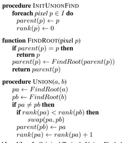
We are introducing here a novel algorithm that avoids this short-coming. It relies on the counting sort algorithm and modifies the un-derlying Tarjan’s Union-Find algorithm (Alg. 1) to store additional information. We recall that this algorithm aims to build a tree struc-ture. Since the tree construction is not a predictive process, some pixels might be put apart before realizing they form the same set. Merging the related subsets is then costly. In order to minimize such a cost, some nodes are identified as having more weight (higher score or rank) than others, and will be selected when two sets are to be merged. Sibling nodes (waiting for being merged) can also be en-countered but the algorithm minimizes the size of siblings that have to be later integrated in the eldest. The tree structure is stored in an array called parents, while the array rank contains scores allowing to choose among the siblings. A fusion step remains mandatory.
In our modified algorithm (Alg. 2, with leader and count used in-stead of parent and rank in Tarjan’s algorithm), we store the number of direct children of a node (set to 1 by default) instead of the so-called rank. When two nodes are linked, either they have the same value and then the one with more children is promoted as leader, or they have different values and then the one with the head value is the parent.
Based on this modified algorithm, we then derive the overall tree construction algorithm (Alg. 3). It relies on a more compact data structure, and involves a new merging strategy. The various optimizations lead to a linear complexity and a memory footprint divided by two. It is a fully parallel algorithm, with only the rein-dexing step requires one image scan and the merging achieved over the tile edges. Initialization (INITBUILDTREE) consists in setting all cells of the parent array to the maximal value. We will later be able to determine if a cell already knows its parent or not. The main construction algorithm (BUILDTREE) relies on a scheduler that will first divide the image surface in as many parts (called tiles) as avail-able processors nbCores. Each tile is then analyzed in parallel to build the related subtree (BUILDSUBTREE). To do so, edges linking neighboring pixels are sorted in ascending order (given a specific metric, related to the kind of tree: min-tree, max-tree), consider-ing the efficient countconsider-ing sort algorithm. Each processor then uses these sorted edges to update leader and count using our modified Union-Find algorithm. When linking two pixels (LINKLEADER), it becomes easy to reach the two roots. Only them are impacted by the change of children and juniors. Through this scan, we also update the direct link to the highest parent at each analysis of a branch. A new node r is created during the first link with a leader pixel (CREATECOMP).
Once partial trees have been computed by each processor, a merging step has to be performed. Let us underline that it may lead to a topology change in the tree, rendering this process particularly costly (see [6]). We thus optimize it by sorting all edges linking border pixels in a raw (second loop in BUILDTREE). The merging
procedure INITUNIONFIND
foreach pixel p ∈ I do parent(p) ← p rank(p) ← 0
function FINDROOT(pixel p) if parent(p) = p then
return p
parent(p) ← F indRoot(parent(p)) return parent(p)
procedure UNION(a, b) pa ← F indRoot(a) pb ← F indRoot(b) if pa 6= pb then
if rank(pa) < rank(pb) then swap(pa, pb)
parent(pb) ← pa
rank(pa) ← rank(pa) + 1
Algorithm 1: Original Tarjan’s Union-Find algorithm
is applied on these edges (MERGEANDCOMPRESS), through a zip-ping that can lead to a topology change in the tree, thus justifying why we are processing smallest edges first. We then assign a new rank for each node (processing all siblings in a raw while reaching the eldest). We finally scan the set of nodes and set them at the ap-propriate location.
We finally add reverse links from the parents to the children (LINEARBUILDCHILDREN). We thus follow a strategy similar to the counting sort. We compute a cumulative sum of children counts and use the underlying array to indicate the first available location and set the children in the children array subsequently.
4. EXPERIMENTS
We report here some experiments conducted in order to assess the performance of the proposed workflow, including the novel tree con-struction algorithm. The underlying architecture is a computation node with 2 sockets L5640 2.27 GHz, 24 dual-cores and 40 GB of RAM. The input data mostly consist of pansharpened VHR optical images coming with a 16-bit resolution.
We consider here an excerpt of a WorldView-3 color (RGB) im-age, of size 9, 250 × 10, 408, i.e. ca. 100 millions of pixels. We append to the original spectral bands some derived features, NDVI and some Sobel indices. Then, a min-tree and/or a max-tree is built from each selected band before computing DAP using some prede-fined thresholds. The feature extraction scheme leads to a feature vector of typical length varying from a few tens to more than one hundered (e.g., computing both a min- and max-tree on the 3 origi-nal bands as well as 2 derived bands, and considering 12 thresholds with a single attribute, leads to 120 features per pixel).
In this example, we have added NDVI as an additional band, as well as the Sobel gradient from NDVI band. We have then com-puted a max-tree only on the NDVI and Sobel bands. The number of thresholds has been limited to 4, thus leading for each pixel to a feature vector of 13 (4 attribute values for each tree and the 5 in-put bands: RGB, NDVI and Sobel on NDVI). As such, the memory footprint of the features has been reduced by a factor of 9, from 21.5 GB to 2.3 GB storage. As far as the CPU time is concerned, we refer the reader to Tab. 4. We can see that the tree construction step is less than 10 seconds per tree (or per band), and the overall
procedure INITLEADER
foreach pixel p ∈ I do leader(p) ← ∞ count(p) ← 1
procedure UPDATELEADER(pixel min, pixel max) while min 6= max do
up ← leader(p) leader(p) ← l p ← up
function FINDUPDATELEADER(pixel p) l ← p up ← leader(l) while up 6= ∞ do l ← up up ← leader(l) U pdateLeader(p, l) return l
function LINKLEADER(pixel max, pixel min, bool eq, pixel a, pixel b)
// max, min are leader pixels of a, b // max is the parent with highest weight // eq is true if both weights are equal if eq AND count(max) < count(min) then
swap(max, min)
count(max) ← eq ? count(min) : 1 U pdateLeader(a, max)
U pdateLeader(b, max) return max
Algorithm 2: Proposed adaptation of Union-Find algorithm
feature extraction step is achieved in about 20 seconds. The train-ing achieved by the Random Forest classifier is performed in less than 5 seconds, considering a set of 15, 000 training samples. With such a low computational cost for feature extraction and training, it is possible to rerun these steps (choosing other bands, attributes or thresholds, providing other training samples) until reaching a satis-fying classification model. Finally, the prediction is done in about 1.5 minute. When including the other steps not given here for the sake of concision (e.g., I/O and memory ops), the land cover map is produced in less than 3 minutes. Let us note that with a stan-dard, single-threaded implementation of the tree-related algorithms, the CPU time would have grown from about 20 seconds to possibly more than 15 minutes (i.e. more than 40x).
Step Total # Min Max Tree construction 17.2” 2 8.4” 8.8” Feature embedding 2.4” 2 1.2” 1.2” Tree filtering 1.9” 2 0.9” 1.0” Training 4.7” 1 – – Prediction 1’30.9” 1 – – Total 2’21.0” – – – Table 1. CPU cost evaluation: total time of each step, number of processes, and min/max CPU times (– when not applicable).
5. CONCLUSION
In this paper, we have addressed the land cover mapping problem at very large scale (e.g., paneuropean). To do so, we have consid-ered as a baseline the popular scheme consisting of DAP feature ex-traction followed by classification using Random Forest. We have then focused on the feature extraction scheme and introduce novel algorithms to lower both the memory footprint and the computa-tional cost, making the proposed implementation compatible with multi-threaded environments. The overall processing chain has been validated by SIRS in an operational context, namely through the mapping of Small woody features (SWF) for EEA39, and is part of the Triskele library, a remote module of the Orfeo ToolBox (OTB) CNES Open Source suite. Let us note that the proposed algorithm aims to be run on a server side, while client access to tree based-structures has been proven to be an effective solution [8].
Future work will include integrating recent DAP extensions (e.g. [2]) in order to improve the classification accuracy, as well as fur-ther investigating computation/memory cost optimization, and ex-perimentally comparing the proposed implementation with existing ones [9, 10].
6. REFERENCES
[1] M. Dalla Mura, J.A. Benediktsson, B. Waske, and L. Bruzzone, “Morphological attribute profiles for the analysis of very high resolution images,” IEEE Transactions on Geoscience and Re-mote Sensing, vol. 48, no. 10, pp. 3747–3762, 2010.
[2] M.T. Pham, S. Lef`evre, and E. Aptoula, “Local feature-based attribute profiles for optical remote sensing image classifica-tion,” IEEE Transactions on Geoscience and Remote Sensing, 2017, to appear.
[3] M. Belgiu and L. Dr˘agut¸, “Random forest in remote sensing: A review of applications and future directions,” ISPRS J. of Pho-togrammetry and Remote Sensing, vol. 114, pp. 24–31, 2016. [4] N. Audebert, B. Le Saux, and S. Lef`evre, “Semantic
segmen-tation of earth observation data using modal and multi-scale deep networks,” in Asian Conference on Computer Vi-sion, 2016.
[5] N. Audebert, B. Le Saux, and S. Lef`evre, “Joint learning from earth observation and openstreetmap data to get faster better se-mantic maps,” in IEEE/ISPRS Workshop on Large Scale Com-puter Vision for Remote Sensing Imagery, 2017.
[6] J. Havel, F. Merciol, and S. Lef`evre, “Efficient tree construc-tion for multiscale image representaconstruc-tion and processing,” Jour-nal of Real-Time Image Processing, pp. 1–18, 2016.
[7] B.B. Damodaran, J. H¨ohle, and S. Lef`evre, “Attribute profiles on derived features for urban land cover classification,” Pho-togrammetric Engineering and Remote Sensing, vol. 83, no. 3, pp. 183–193, 2017.
[8] F. Merciol, A. Sauray, and S. Lef`evre, “Interoperability of mul-tiscale visual representations for satellite image big data,” in ESA Conference on Big Data from Space, 2016.
[9] E. Carlinet and T. G´eraud, “A comparative review of com-ponent tree computation algorithms,” IEEE Transactions on Image Processing, vol. 23, no. 9, pp. 3885–3895, 2014. [10] J. Kazemier, G. Ouzounis, and M. Wilkinson, “Connected
morphological attribute filters on distributed memory parallel machines,” in International Symposium on Mathematical Mor-phology, 2017, pp. 357–368.
procedure INITBUILDTREE(Image I) foreach pixel p ∈ I do
parent(p) ← ∞
procedure BUILDTREE(Image I) tiles ← tileImage(I, nbCores) foreach tile ∈ tiles do in parallel
BuildSubT ree(tile, I)
borders ← borderImage(I, tiles) foreach border ∈ borders do in parallel
borders(border) ← getSortedEdges(I, border) M ergeAndCompress(borders)
LinearBuildChildren() procedure BUILDSUBTREE(tile, I)
edges ← getSortedEdges(I, tile) foreach e ∈ edges do ra ← F indU pdateLeader(e.a) rb ← F indU pdateLeader(e.b) if ra = rb then continue wa ← value(ra) wb ← value(rb) if wa < wb then swap(ra, rb) r ← LinkLeader(ra, rb, wa == wb, la, lb) par ← CreateComp(r, value(e), count(r)) if ra 6= r then
linkP arent(ra, par) if rb 6= r then
linkP arent(rb, par)
function CREATECOMP(leader, level, size) par ← parent(leader) if par = ∞ then par ← nbComp++ parent(leader) ← par compLevel(par) ← level nbChild(par) ← size return par
procedure MERGEANDCOMPRESS(borders) foreach e ∈ borders do
connectLeaf (e.a, e.b, value(e)) newRank ← 0
foreach e ∈ tiles do f indU pdateT op(e)
parN ewP os(e) ← newRank++ foreach pos ∈ comp do
swap(parent(pos), parent(parN ewP os)) procedure LINEARBUILDCHILDREN()
sum ← 0 foreach comp do
sum ← sum + nbChild(comp) nbChild(comp) ← sum posChild ← nbChild foreach x ∈ leaf and comp do
par ← parent(x) − 1 pos ← posChild(par) pos++
posChild(par) ← pos children(pos) ← x
// first child : children(nbChild(par − 1)) // last child : children(nbChild(par))