HAL Id: hal-00913620
https://hal.archives-ouvertes.fr/hal-00913620v2
Submitted on 3 Jun 2014
HAL is a multi-disciplinary open access archive for the deposit and dissemination of sci-entific research documents, whether they are pub-lished or not. The documents may come from teaching and research institutions in France or abroad, or from public or private research centers.
L’archive ouverte pluridisciplinaire HAL, est destinée au dépôt et à la diffusion de documents scientifiques de niveau recherche, publiés ou non, émanant des établissements d’enseignement et de recherche français ou étrangers, des laboratoires publics ou privés.
Simultaneous High Dynamic Range and
Super-Resolution Imaging Without Regularization
Yann Traonmilin, Cecilia Aguerrebere
To cite this version:
Yann Traonmilin, Cecilia Aguerrebere. Simultaneous High Dynamic Range and Super-Resolution Imaging Without Regularization. SIAM Journal on Imaging Sciences, Society for Industrial and Applied Mathematics, 2014, pp.7(3), 1624-1644. �10.1137/130946903�. �hal-00913620v2�
Regularization
Yann Traonmilin†and Cecilia Aguerrebere† ‡
Abstract. Modern digital cameras sensors only capture a limited amplitude and frequency range of the irradi-ance of a scene. A recent trend is to acquire and combine multiple images to raise the quality of the final image. Multi-image techniques are used in high dynamic range processing, where multiple ex-posure times are used to reconstruct the full range of irradiance. With multi-image super-resolution, the difference between sampling grids caused by the motion of the camera is used to generate a high resolution image. It is possible to combine these two processes into one to generate a super-resolved image with a full dynamic range. In this paper, we study the reconstruction error of high dynamic range super-resolution imaging without regularization, under affine motion hypothesis. From this study, we deduce a strategy for the choice of the number of images and the exposure times which makes the unregularized problem well conditioned. With these acquisition parameters, if the affine motion hypothesis holds and sufficiently long exposure time is available, the recovery of all the amplitude and frequency content of the scene irradiance is guaranteed.
Key words. super-resolution, high dynamic range, regularization
1. Introduction. Limitations of digital cameras sensors restrict the information that a single image can possibly gather. In particular, the spatial sampling and the dynamic range of an image are limited. Restrictions on spatial sampling result in aliased images. Scenes with high dynamic range have over or under-exposed image regions because of the sensor’s limited potential well capacity. A way to overcome these two problems is to improve spatial and dynamic range sampling by acquiring and combining several images of the scene. Motion between shots gives a spatial sampling diversity that allows for a high resolution reconstruc-tion of the scene. The process of recovering a high resolureconstruc-tion (HR) image from several low resolution (LR) ones is called super-resolution imaging (SR). The dynamic range limit can be extended by using different exposure times or gains between images. This process is called high dynamic range imaging (HDR). These two processes need to be combined in order to recover the high frequency and high dynamic range information of the scene.
Super-resolution algorithms have been reviewed in several works [10,20,33]. Most of them can be summarized with a variational approach. The HR image is recovered by minimizing a regularized data-fit functional. This data-fit is usually an Lp norm fit. From Tychonov to total
variation, many regularization functionals are available. Such regularization is necessary when little information is available (i.e., a small number of images). The resulting interpolation must be considered as an inpainting using a regularity model and not as the recovery of missing high frequency information as the scene might not verify the regularity hypothesis. It has been shown [7,35] that regularization becomes less useful when a large number of images are available. It is then possible to reconstruct the real high frequency content of the acquired
†LTCI CNRS & T´el´ecom ParisTech, 75634 PARIS Cedex 13, France. [email protected]
‡Instituto de Ingenier´ıa El´ectrica, Facultad de Ingenier´ıa, Universidad de la Rep´ublica, Montevideo,
Uruguay.
scene by minimizing only the L2-norm data-fit.
Several HDR image generation algorithms have been proposed since the seminal work by Mann and Picard [19]. For static scenes, when the input images can be perfectly registered, the irradiance at each pixel is computed as a weighted average of the corresponding samples acquired with different exposure times or gains. Based on this idea, several methods have been proposed following different weighting schemes [2,9,12,16,18,21,26]. However, accurate realignment of aliased images is difficult because it is impossible to correctly apply a geometric transformation to well-sampled details and aliased patterns at the same time. Thus a joint HDR-SR method is needed.
In recent years, some algorithms have been proposed to perform SR and HDR simultane-ously. The most conventional approach is to use a weighted least squares scheme, as normally done for SR, but on the irradiance [8,14] or transformed irradiance domain [6]. A different approach [38] is to align LR images using optical flow and minimize a regularized energy to achieve the combined HDR-SR reconstruction. Rad et al. [4] propose to first align the in-put images and then use a Delaunay triangulation and bi-cubic interpolation to perform the HDR-SR estimation on the irradiance domain. The combined problem has also been stud-ied from a sensor design perspective, with proposed solutions based on specifically adapted sensors [23,24].
An aspect common to all these methods is the use of a regularization term, which threatens multi-image super-resolution in terms of high frequency recovery capability. The recovery of the spectrum of the real HR scene cannot be guaranteed. Moreover, the latest results for HDR image generation [2], such as the near optimality of the weighting scheme proposed by Granados et al., are not exploited. To the best of our knowledge, the theoretical background of this problem, necessary to ensure the recovery of HDR and HR content, has not been studied in depth.
1.1. Contributions. In this paper, we study the HDR-SR imaging problem from the fol-lowing perspective: which image acquisition configuration, i.e. number of acquired images and exposure times, guarantees that the high frequencies and the full dynamic range of a scene will be recovered? We use a realistic camera acquisition model with affine motion hypothesis and propose an image reconstruction method that includes the weighting scheme shown to be nearly optimal for HDR information recovery [2]. We study theoretical bounds for the joint HDR-SR reconstruction error and find that a trade off must be made between the to-tal exposure time and the number of images. This result is illustrated with synthetic and real data experiments. Moreover, we show how exposure times can be selected and that this selection can be decoupled from the SR problem to fulfill our objective. This analysis leads to the proposal of an acquisition strategy which, if the affine motion hypothesis holds and sufficiently long exposure time is available, guarantees the recovery of the full dynamic range and high frequency content of the scene irradiance. Finally, experiments with real data show that our HDR-SR strategy manages to recover this information.
The article is organized as follows. Section 2 introduces the image acquisition model and the reconstruction method. In section 3, the strategy for the choice of exposure times and number of images is presented. Section 4 is devoted to the study of the reconstruction error bounds. In Section 5, we show how exposure times can be selected. An optimal acquisition
strategy and its corresponding experimental validation are presented in Section 6. Finally, conclusions are stated in Section 7.
2. HDR-SR acquisition and reconstruction.
2.1. Acquisition model. We consider a monochromatic irradiance acquisition model with different exposure times for each raw low resolution image wi(we suppose that they are square
of size l × l). The acquisition operator A is defined as
A : RM l×M l→ RN ×(l×l)
u → (wi)i=1,...,N = (ΩiGiSQiu)i=1,...,N,
(2.1)
where N is the number of LR images, u ∈ RM l×M l is the HR irradiance of size M l × Ml, Qi ∈ R(M l×M l)×(M l×M l) are the affine motions associated with each LR image (Qiu is the
irradiance reaching the sensor), S ∈ R(l×l)×(M l×M l)is the sub-sampling by a factor M (M can be called the super-resolution zoom or factor) and Gi ∈ R(l×l)×(l×l), Gi = gti is the overall
acquisition gain, including the camera gain g (without loss of generality, we take g = 1 to simplify expressions) and the exposure time ti for the i-th LR image. Several images may be
acquired with the same exposure time. Ωi∈ R(l×l)×(l×l) is a diagonal matrix taking value 1 if
pixel j does not become saturated or under-exposed for the exposure time ti and 0 otherwise.
We suppose Ω = (Ωi)i=1,...,N to be full rank (every pixel is at least illuminated once). This
model is close to the one introduced in [14]. We use a simplified version of it in order to facilitate the study. Unlike [14], the camera response function is here considered to be linear, which is a realistic model for raw images [12]. Our model does not take into account the point spread function of the camera, which can be deconvolved afterward if motion is small [34]. The quantization error is neglected as, except in very low light conditions, it is small compared to the readout noise variance nR [2]. As we consider a monochromatic acquisition model, the
Bayer pattern is ignored. With our model, the production of a demosaicked color HR image without regularization, would take the form of a separate inversion of the 3 color channels. Only the motion due to the shift in the grid would have to be included in Qi. Note that the
green channel would have 2 times more LR images than red and blue channels. The digital LR images w = (wi)i=1,...,N are contaminated by additive noise n:
(2.2) w = Au + n.
A Poisson noise model with Gaussian approximation [1] leads to the spatially varying Gaussian noise
(2.3) n = nu+ nR,
where nu is a Gaussian noise with covariance matrix Σu proportional to the irradiance (Σu =
diag(Au)) and nRis a Gaussian readout noise with constant variance σ2R. Thus the covariance
matrix of n is Σ = diag(Au) + σ2RI (I = identity matrix). The objective is to recover u from w.
2.2. Image reconstruction. It has been shown in [35] that M2 images are necessary to
perfectly recover the HR image in the case of constant exposure times. Because we supposed that the HDR acquisition model is a full rank linear map, the composition of the two processes is invertible with M2 LR images. We minimize the L2 data-fit to recover an estimate of u
(2.4) u = argmin˜ ukW1/2(Au − w)k22.
Multiplying by W1/2= Σ−1/2normalizes the noise to have constant variance, thus the solution to (2.4) gives the minimum variance linear unbiased estimator of the irradiance. Practically, this problem is solved with a linear conjugate gradient calculation of (W1/2A)†W1/2w =
(AHW A)−1AHW w. Since the weights W depend on the irradiance u, an iterative procedure is needed to complete the estimation. The weights can be initialized with a smoothed version of the LR images. In practice, it is found that one iteration yields good results, and the irradiance remains almost unchanged after the first iteration. The iterative computation of this estimator for the HDR image generation in the case of perfectly registered images, is introduced by Granados et al. [12] and shown to be nearly optimal in [2].
If Ωi= I, Gi = I and W = I (no HDR in the model), Equation2.4is the conventional L2
super-resolution reconstruction procedure.
An experiment is conducted to evaluate the benefit of using the weights W . For this purpose, synthetic samples are generated from a ground-truth HDR image according to model (2.2), and the reconstruction is performed solving (2.4), with W1/2= Σ−1/2and W = I.
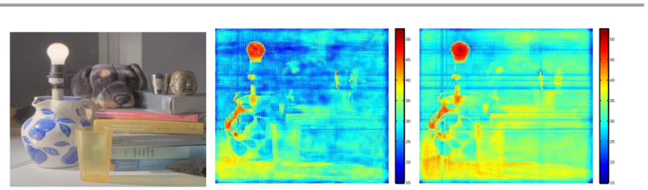
The experiment is repeated 100 times, with randomly chosen affine transformations and noise realizations. The signal-to-noise ration (SNR) for each reconstructed pixel is computed from the ground-truth value and the mean square error (MSE) at that pixel (MSE computed from the 100 experiments). Figure 2.1 shows the SNR images in decibels for each weighting type. The results greatly improve when the weights W1/2= Σ−1/2 are included. The improvement (gain in SNR) is more remarkable in the darker regions of the scene where the input samples are noisier. An average gain of 3.9 dB (average SNR for all pixels) is found comparing the cases with weights (32.5 dB) and without weights (28.6 dB).
2.3. Image registration. Image registration is a critical part of SR as the quality of the result will be directly linked to the precision of motion estimation. With low resolution images, registration can be inaccurate [29]. For super-resolution, high resolution motion estimation is often performed with the variable projection method [11,28,31,37]. It has been shown that this method gives good results when enough images are available [34]. We adapt this method to our joint HDR-SR reconstruction problem. For a given HDR setting (Ωi and Gi known),
let A(θ) be a SR operator parametrized by the affine motion parameter θ ∈ R6N and ˜u(θ) the solution of (2.4) with operator A(θ). The variable projection aims at finding the minimizer (2.5) θ˜ = argminθkW1/2(A(θ)˜u(θ) − w) k22.
It is a non-linear non convex functional having local minima. From an initial solution, we perform a conjugate gradient descent of functional (2.5).
The initial solution is calculated as follows. We calculate the cross-correlation of each LR images pair for different translations and find the translation maximizing the cross-correlation. We remark that the translation τij between images i and j should be the sum of the translation
15 20 25 30 35 40 45 50 15 20 25 30 35 40 45 50
Figure 2.1. Result of optimal reconstruction for HDR-SR. SNR for each pixel obtained from 100 experi-ments with randomly chosen affine transformations and noise realizations. Left: Ground-truth image from [15].
Center: SNR obtained without weights (W = I). Right: SNR obtained using W1/2
= Σ−1/2. The
improve-ment is more remarkable in the darker regions of the scene where the input samples are noisier. An average gain of 3.9 dB (average SNR for all pixels) is found comparing the cases with weights (32.5 dB) and without weights (28.6 dB).
τik between images i and k and translation τkj between k and j. Then, to obtain the final
translation to the reference image, we average all the available τ1k+ τkj. We then scan for
initial rotation and zoom to avoid local minima.
3. Strategy for the choice of acquisition parameters. In order to establish an HDR-SR reconstruction strategy, we must define the set of exposure times and the number of images (per exposure time) to acquire. Given a set of exposure times t1, . . . , tN, the reconstruction
error can be arbitrarily large because the condition number of the acquisition operator A cannot be bounded. For instance, it is infinite if the camera does not move (Qi = I). Therefore,
it is not possible to find the exposure times minimizing the reconstruction error for the HDR-SR combined problem without knowledge of the camera motion. In practice, the motion is seldom known. In particular, it is unknown for images acquired with a hand-held camera.
Performing a joint optimization of exposure times and number of images for HDR-SR would require a precise statistical model describing camera motion. Even with this informa-tion, calculating precise estimates of the reconstruction error would be difficult because we would have to estimate the interaction between the local conditioning of super-resolution [35] and the spatial variations of the SNR. Moreover, this joint problem is a highly dimensional non-convex problem, which would be hard to embed in a camera.
Hence, we propose to define a reconstruction strategy combining the optimality results for each separate problem, HDR and SR, so as to minimize the worst case reconstruction error of the combined problem. With HDR processing, we know that parts of the images are illuminated by few images. From SR theory, these parts must be covered by enough images to enable a reconstruction without regularization. Consequently, we proceed as follows.
Proposed strategy. For the HDR reconstruction problem, an optimal HR HDR image is obtained if p HR images with exposures t1, . . . , tp are combined, these exposures being chosen
to minimize the HDR reconstruction error (c.f. Section 5). Hence, we propose to consider the SR conditions which best estimate each of these p HR images. This will guarantee that the joint HDR-SR reconstruction performs well.
with that exposure that lead to a good SR reconstruction of the p HR images. Then a naive linear HDR-SR method would be to perform a classical HDR technique, with these p reconstructed HR images, thus limiting the final reconstruction noise. But we know that our joint method (minimization (2.4)) leads to the optimal L2 reconstruction error, given this
dataset. Consequently, by minimizing the reconstruction error of the separate HDR and SR problems, we guarantee a good reconstruction error for the joint HDR-SR problem.
Given a set of exposure times t1, . . . , tp that minimize the HR HDR reconstruction error,
two cases are to be considered. First, if the total exposure time and the total number of images are not limited, the best strategy for each exposure (ti)i=1,...,pis to take as many LR images as
possible with this exposure in order to improve the SR reconstruction. With equal exposure times, the problem becomes a pure super-resolution problem where more images improve the quality of the reconstruction [7,35]. Longer exposures are not desirable since they increase the number of saturated pixels thus increasing the reconstruction error. Secondly, a more realistic case, is that of a limited total exposure time (e.g. because of scene motion). In order to ensure a correct HR reconstruction with a super-resolution factor (or zoom) M , the minimum total exposure time for frames acquired with time ti is M2ti. However, as it will be shown in the
following section, there is an optimal number of LR images N > M2 for a fixed total exposure
time.
4. Reconstruction error bound for HDR-SR. In the following section we study the recon-struction error bounds for the HDR-SR estimation problem for a fixed total exposure time T and N images acquired with equal exposure T /N , i.e. the reconstruction of the HR irradiance frame.
4.1. Optimal number of images for a fixed total exposure time. In a HDR context, when neglecting motion blur, the longer the exposure time without saturation, the better. We show here that when we must perform SR at the same time (i.e. compute the pseudo-inverse of A), taking more images with a shorter exposure can be better. We study the case of HDR-SR for a given total exposure time T without saturation, i.e. Ωi = I. N images are
acquired with a total exposure time T , each with equal exposure time t = T /N . Because the overall acquisition gain is linear, the problem is equivalent to the acquisition of N LR irradiances v with A′ = G−1A, with a noise n′ with covariance matrix:
(4.1) Σ′= diag(A′u/t + σ2R/t2). Then,
(4.2) v = A′u + n′.
A′ is the conventional super-resolution modeling operator, i.e. a super-resolution operator
where acquisition gain is not considered. Thanks to this normalization, we will be able to use results from the super-resolution literature directly.
The super-resolution of N images with exposure T /N can be done solving the problem (4.3) u = argmin˜ vkW′1/2(A′u − v)k22,
Reconstruction error bound. The noise in the reconstructed image nrec is thus bounded by (c.f. AppendixA) (4.4) knreck22 ≤ κ(N )2 σ2 max(A′) m2l2 ˜ m (1 + rN )N 2,
where κ(N ) is the conditioning of A′HA′ (ratio of extremal eigenvalues of A′HA′), σ
max(A′)
is the maximum singular value of A′, m = sup(u) ⋍ sup(A′u), ˜m = inf(u) ⋍ inf(A′u),
r = σR2/(T m), ˜r = σR2/(T ˜m) and l is the size of the input images. Hence, the optimal number of images for a fixed total time T is the one that minimizes knreck2.
In [35], it was shown that κ(N ) can be bounded in probability by a decreasing function of the number of images N . Moreover, it can be shown [36] that N/M2 ≤ kA′k2
2 = σmax2 (A′) ≤ N.
Hence, to optimize the reconstruction error bound, we minimize the function (4.5) f (N ) = κ(N )2(1 + rN )N,
with respect to N . When N is close to the critical case M2, κ(N ) can be large but decreases
to 1 with N [35]. The conditioning of the SR operator has been also studied extensively in [7,30]. Consequently, f will have a minimum. Notice that the r factor is proportional to σ2
R and cannot be neglected in low light conditions. If we added saturation for a particular
time T /N0 with N0 ≥ M2, the bound would still be valid for N > N0. For N ≤ N0, matrix
A′ is not invertible, thus the error is not bounded.
4.1.1. Experimental study of f (N ).
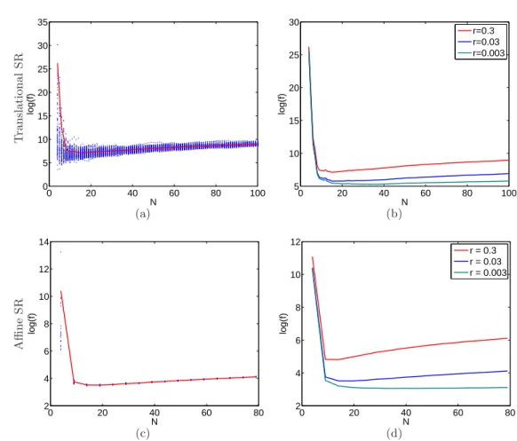
Synthetic data. To illustrate the behavior of f (N ), we compute the curve for the case of 2D translational super-resolution. For each number of images N , we randomly simulate 100 translation parameters and compute the corresponding f (N ) by explicitly calculating κ(N ) (which can be done because the SR is then a 2D Vandermonde system in the frequency domain [3,25]). With the same procedure, we generate the f (N ) curve for the affine super-resolution case. Here κ(N ) is approximated by the ratio knreck2/knink2. Figure4.1shows the
results obtained with M = 2 and r = 0.03 (chosen with realistic values: σ2R = 30, T = 1/10, m = 104).
It can be verified that the minimum of f is not reached at the critical case (N = M2= 4), meaning that it is better to take more than M2 images with shorter exposure times. This fact
shows that a compromise must be made between the number of images needed to perform super-resolution (more than M2) and the noise level on those images. Given the total exposure time T , a degradation of the performance can be observed for large N . This can be explained by the fact that each image has a shorter exposure time. For short enough exposures, the variance σ2R of the readout noise becomes prominent. The amount of noise in LR images becomes too big to be compensated by the averaging effect of super-resolution, thus increasing the reconstruction error.
This can be verified with the results obtained for various r values in Figure 4.1. The r factor can be thought of as the inverse of the dynamic range of the acquired scene, since it is equal to the ratio between the constant noise variance σ2R and the maximum acquired irradiance mT (up to the factor N ). As the value of r decreases, the minimum of f (N ) is
T ra n sl a ti o n a l S R 0 20 40 60 80 100 0 5 10 15 20 25 30 35 N log(f) (a) 0 20 40 60 80 100 5 10 15 20 25 30 N log(f) r=0.3 r=0.03 r=0.003 (b) A ffi n e S R 0 20 40 60 80 2 4 6 8 10 12 14 N log(f) (c) 0 20 40 60 80 2 4 6 8 10 12 N log(f) r = 0.3 r = 0.03 r = 0.003 (d)
Figure 4.1. Plot of log(f (N )) versus N (M = 2). (a) Result for 100 experiments (blue) and average (red) of 2D translational SR for each N with r = 0.03 . The minimum is reached at N = 12 . (b) Plot of the average log(f ) for different values of r for translational SR. Minimum at 12 (r=0.3), 13 (r=0.03) and 30 (r=0.003). (c) Affine super-resolution, 20 experiments for each N . The minimum is reached at N = 19, (d) Plot of average log(f (N )) versus N for different values of r for affine SR. Minimum at 14 (r=0.3), 19 (r=0.03) and 34 (r=0.003).
reached at a larger N . This is due to the fact that both, decreasing σR2 or increasing T , improves image quality and thus allows the use of shorter exposure times. Moreover, notice that the error bound increases quite slowly after its minimum. Hence, whether we choose a number of images at the minimum or slightly above will have little impact on the results. Curves of similar shape are obtained for larger M values, with the minimum reached for a larger N . This is caused by the larger conditioning of the SR problem for larger M [5].
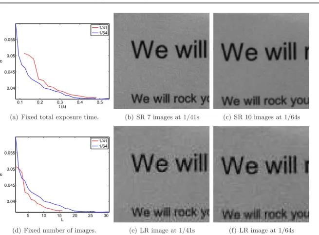
Real data. In order to experimentally verify the previous results, we take pictures of a planar surface using a hand held camera (c.f Figure 4.2). The small hand motion gives the sampling diversity needed for HDR-SR and guarantee that motion blur is not too large. The goal is to compare the HDR-SR reconstruction error (M = 2) obtained with a constant total exposure time T , but with two different exposure times, t1 = 1/41 and t2= 1/64, i.e. with a
0.1 0.2 0.3 0.4 0.5 0.04 0.045 0.05 0.055 t (s) σ 1/41 1/64
(a) Fixed total exposure time. (b) SR 7 images at 1/41s (c) SR 10 images at 1/64s
5 10 15 20 25 30 0.04 0.045 0.05 0.055 L σ 1/41 1/64
(d) Fixed number of images. (e) LR image at 1/41s (f) LR image at 1/64s
Figure 4.2. Reconstruction error with respect to total exposure time and number of images (M = 2). (a) Reconstruction error with respect to total time. (b) Reconstruction error with respect to number of images. (c) SR result with 7 images at 1/41s. (d) One LR image with exposure 1/41s. (e) SR result with 10 images at 1/64s. (f ) one LR image at with exposure 1/64s.
are compared for the two different exposure times when fixing the total number of images N , i.e. for a different total exposure time N t1 and N t2 in each case. The reconstruction error
(estimated from the variance of gray parts) with respect to the total exposure time and the number of images, for the two different exposure times, is shown in figures 4.2 (a) and (d) respectively. In this example, for a fixed number of images, it is better to take pictures at 1/41 seconds. However, for a fixed total exposure time, it is better to combine more images with the shorter exposure 1/64 seconds. The same behavior can be observed in the extracts of the reconstructed images shown in figures 4.2(b) and (c). Hence, we verify that the longest exposure time is not necessarily optimal.
4.2. Discussion and practical consequences. In this section, we explain the trade off that must be made when performing HDR and SR simultaneously: in an HDR setting, we look for the biggest exposure times which do not saturate (or saturate for the fewest images possible) while with SR, more images are generally better. This leads to the following remarks depending on the acquisition setup:
case for SR (M2), thus with a shorter exposure. However, it must not exceed by much
the critical case since for very short exposures the reconstruction noise increases with N .
• With a fixed number of images, the more images with the longest possible exposure time the best. However, the previous remark give us the knowledge that if this number of images is the optimal one from the previous section, then it is not possible to do better with the same total exposure time.
• With any exposure time / number of images, the best strategy is taking as much images as possible of the longest exposure time. Taking a lot of images with very short times is not a good strategy.
5. Exposure times selection for HDR reconstruction. The selection of the exposure times is a key aspect of the HDR imaging problem. Several approaches can be found in the literature that tackle this problem from different perspectives. Some of the proposed methods look for the optimal times set that ensures that a predefined dynamic range will be captured [13,22]. Another group of methods focuses on the quality of the reconstructed HDR image and optimizes a risk function that depends on the mean squared error [17] or the signal to noise ratio of the reconstruction [12,16]. These methods need a prior estimation of the scene irradiance, which is assumed to be available for instance through the irradiance histogram.
In this work, we focus on the minimization of the HDR-SR reconstruction error, and we seek for the exposure times set that minimizes the HDR reconstruction error for a given number of exposures N′. The determination of the number of different exposure times N′
is an important problem in HDR imaging, since it has a major impact on the quality of the results and on the practical constraints of the acquisition. Given that it is not the goal of this work to study this problem, we consider instead the value N′ as a given parameter, which
might eventually be set from the known irradiance histogram. An histogram of the scene irradiance is assumed known. In this section we concentrate on the extension of the dynamic range of the image (M = 1, Qi = I, S = I) and propose an algorithm to find this exposure
times set.
In this case, the solution to equation (2.4) gives the following estimator of the irradiance at position j: (5.1) u˜j = PN′ i=1 tiΩijwij ujti+σ2R PN′ h=1 t2 hΩhj ujth+σ2R .
Thus the irradiance estimator variance in this case is given by
(5.2) knreck22= l2 M2 X j=1 1 PN′ h=1 t2 hΩhj ujth+σR2 .
Then, we consider the optimal set of times as the one that minimizes (5.2).
If we neglect the readout noise variance σ2R, the irradiance estimator variance expressed in (5.2) depends on the square root of the signal √uj. Thus, the minimization of (5.2)
0 0.1 0.2 0 0.05 0.1 0.15 0.2 0 1 2 3 x 10⁻⁷ t 2 t 1
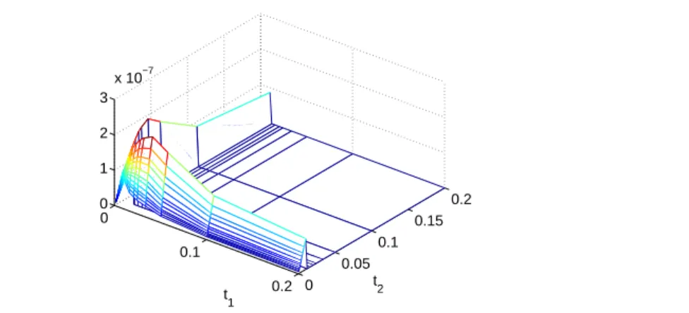
Figure 5.1. Inverse of the normalized reconstruction error (inverse of Equation (5.3)) for the first example scene of Section 6.
signal as a way to counter this dependence and prioritize noise reduction in low light pixels, since noise is generally amplified in those pixels by post-processing tone mapping techniques used to display HDR images. Several tone mapping techniques perform a contrast reduction of the irradiance image that magnifies the noise visibility mainly in dark regions [27]. Nev-ertheless, this is clearly one possible option among multiple valid options. Other approaches are also valid (e.g. normalization by the squared signal u2j so as to minimize the squared sig-nal to noise ratio) and may be incorporated into the proposed HDR-SR acquisition strategy by modifying (5.2) accordingly. Therefore, we consider the normalized irradiance estimator variance (5.3) kn′ reck22 = l2 M2 X j=1 1 uj PN′ h=1 t2 hΩhj ujth+σ2R = l2 M2 X j=1 1 PN′ h=1 t2 hΩhj th+σR2/uj ,
and the set of exposure times
(5.4) ˜t1, . . . , ˜tN′ = arg min
t1,...,tN′kn
′ reck22.
To minimize the non-convex function (5.3), we propose to use an exhaustive evaluation method. First, the shorter exposure time is determined by the fact that all irradiance values must be correctly acquired for at least one exposure time (matrix A is full rank). For the same reason, a lower bound is determined for the longer exposure. Then, given the number N′ of
exposure times to acquire (which might be automatically extracted from the scene histogram), we need to minimize function (5.3) with respect to the remaining N′− 1 times. We find this
minimum by evaluating all combinations of available times. This methodology is feasible and fast in practice since N′ is usually in the order of 2 to 4 and the number of available exposures in the camera is about 50 (e.g. 55 for the Canon 7D).
Figure 5.1 shows the inverse of function (5.3) for the example scene presented on the first experiment of Section 6 with N′= 2. The large flat region for the longer exposure times represents the large error caused by the saturation of most (or all) pixels in the image. A large error is also found for very short exposure times, since the readout noise becomes important
for all irradiance values. The maximum of the function (minimum of (5.3)) is reached between these two extremes, as a compromise between saturation and noise level. This compromise is determined from the proportion of pixels belonging to each irradiance range, which is derived from the irradiance histogram of the scene.
6. Acquisition strategy. From the results presented in previous sections we derive the following strategy for the a regularized HDR-SR reconstruction that guarantees the recovery of the amplitude and frequency content of the scene irradiance. The exposure times are first selected following the procedure introduced in section 5. For this purpose, two images are taken to compute the histogram of the scene irradiance and find the optimal exposure times for the HDR reconstruction. One image must capture bright regions (no saturated pixels) and the other must capture dark regions (no under-exposed pixels). From the concatenated histograms of the two exposures, the high dynamic range histogram of the irradiance is built. With this histogram, the minimization from equation (5.4) is performed for the given number of exposure times.
The number of images to take for each exposure time is thus defined from the study presented in section 4. It should be taken as the minimum of function f according to the second remark in section 4.2. The function f , thus the optimal N , depends on the scene irradiance. However, for M = 2, we find in practice that it is reached at about N = 20 for a large range of irradiances. It can be larger for smaller r values, but in those cases the function is quite flat and the result is not greatly affected by this choice. Because N = 20 is a feasible number of shots for burst acquisition with a hand-held camera, it can be taken as the reference number of images needed for each exposure time. Hence, 20 hand-held pictures are taken for each of the selected exposures and the joint HDR-SR is performed solving (2.4) with all images. As stated in Section3, the joint HDR-SR reconstruction gives the minimum L2 reconstruction error and is thus preferable over the separate reconstruction (super-resolution for each HDR exposure and then HDR imaging to combine the HR frames). Moreover, separate registration for times which saturate a large part of the image can fail (e.g. the series of images from 6.4
(c) (f)).
6.1. Experiments. The following experiments were conducted in order to test the capacity of the proposed strategy to recover the dynamic and frequency information lost by a single image acquisition without the need of regularization hypothesis on the scene. To be as close as possible to our model we used the raw images from a high end commercial camera for real data experiments (second and third experiments)
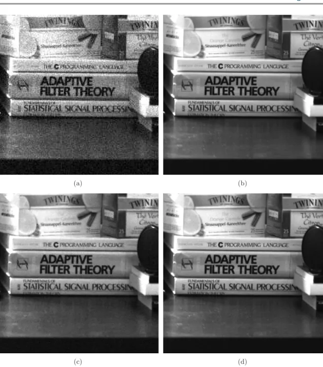
Synthetic data. In the experiment of Figures 6.2 and 6.3, we illustrate how taking the advocated number of images yields a better reconstruction than a total variation (TV) regu-larization [32] with less images. We generate synthetic LR images, according to Model (2.2), from an HR irradiance map (extracted from a real scene). For TV regularization, we generate 2 LR images at the three exposure times 641 , 411 and 321 seconds. We add a total variation regularization term to minimization (2.4) and choose the regularization parameter giving the best PSNR. For the unregularized case, we generate 20 images for each of these times, and perform minimization (2.4). The difference in reconstruction quality can be noticed both qualitatively, and in terms of PSNR. The unregularized version has a 6dB PSNR improve-ment, and the content of the image is not altered (frequencies are not distorted). The TV
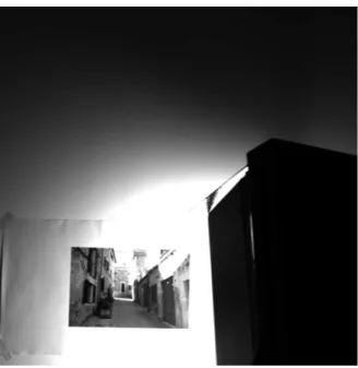
Figure 6.1. A picture of the practical set-up of our first experiment
regularized method alters edges, as for example in the small text areas.
High dynamic range planar surface. We use a planar surface half illuminated by a strong source, thus generating two levels of irradiance. The scene is shown in Figure6.1. Acquiring a plane matches the hypothesis of affine motion (small homography). In a more complex scene, segmenting the image in parts where the affine motion hypothesis is valid might be necessary. The strategy introduced in section 6 is used first to find the 3 optimal exposure times (which are enough to capture the two different illumination levels of the scene) for the scene:
1
100, 801 and 321 seconds. Then, 20 hand-held pictures are taken for each of the three selected
exposures (total exposure time is approximately 1.1 second). Finally, the joint HDR-SR is performed solving (2.4) for all images.
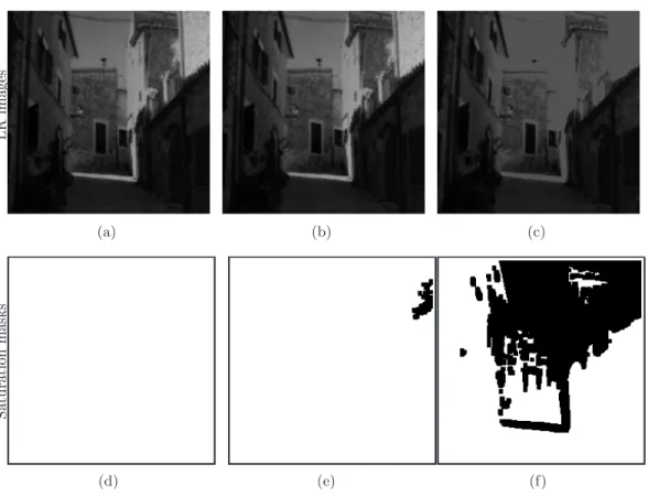
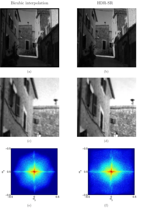
Figure 6.4shows example images for each exposure time in the irradiance domain (i.e. at the same scale) along with the corresponding saturation masks. We observe the increasing saturation for increasing exposure time. In Figure6.5, the result of the HDR-SR reconstruction with factor M = 2 is displayed along with the result of a bi-cubic interpolation of the reference image for comparison purposes. All images are at the appropriate scale for a fair comparison. As expected, the HR image resulting from HDR-SR reconstruction is sharper and less noisy than the bi-cubic interpolation. In this practical case, the intrinsic frequency content of the scene is not very rich because the camera has a physical anti-aliasing filter that cuts much of the high frequencies. However, the recovery of higher frequency information (which does not rely on any regularity model of the scene) is visible, especially on the plot of frequency spectra.
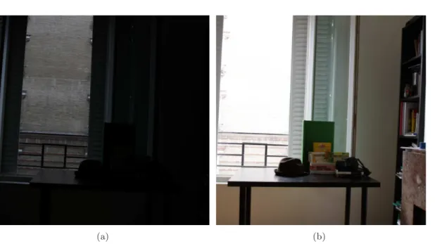
Complex scene. An HDR-SR experiment was conducted in the scene shown in Figure6.6. The strategy introduced in section 6 is used to find 3 optimal exposure times for the scene:
1
(a) (b)
(c) (d)
Figure 6.2. Comparison between regularization with few 6 images and without regularization with 60 images, (a) One of the LR images, (b) HR image, (c) optimal TV regularization with 6 images, (d) SR without regularization and 60 images. See details in Figure 6.3.
exposures. The total exposure time is approximately 1.4 seconds. In order to apply (2.4), the HDR-SR reconstruction must be performed in sub-regions of the images verifying the affine motion hypothesis. The joint HDR-SR for each region is performed solving (2.4) from the corresponding regions of all input images. Figure 6.7shows the HDR-SR reconstruction for a bright and a dark region of the scene. The recovery of high resolution content is particularly
(a) (b)
(c) (d)
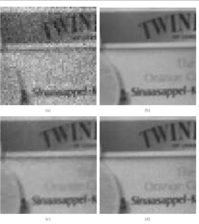
Figure 6.3. Detail of Figure6.3. (a) One of the LR images, (b) HR image, (c) optimal TV regularization with 6 images, PSNR=43.48dB, (d) SR without regularization and 60 images, PSNR=49.92dB.
visible in the focused part of the image (see figures 6.7(d) and 6.8 ). In particular, the aliasing in the LR image (noticeable on the text) is greatly reduced in the reconstruction. The improvement is less noticeable in the bright region (see figure 6.7(b)) since that part of the image is out of focus.
L R im a g es (a) (b) (c) S a tu ra ti o n m a sk s (d) (e) (f)
Figure 6.4. Acquired LR irradiance images with different exposure times with their respective saturation masks (saturated parts are in black) (a) reference image at 1
100, (b) image at 1
80, (c) image at 1
30, (d) saturation
mask for image (a), (e) saturation mask for image (b), (f ) saturation mask for image (c).
7. Conclusions. In this work, we exposed how the HDR-SR problem can be set-up as a minimization problem including state of the art techniques from both sides of the problem. We showed that particular care is necessary when choosing acquisition parameters for high dynamic range super-resolution. A balance between noise generation due to the conditioning of super-resolution and the noise intensity corresponding to the length of exposure times should be found. We also showed how exposure times for HDR-SR can be chosen. The main conclusion of this work is the suggested strategy which ensures that, if the affine motion hypothesis holds and sufficiently long exposure time is available then all the information contained in the irradiance scene (both in amplitude and in frequency) is recovered.
A. Reconstruction error bound. Computation of the reconstruction error bound for the weighted least squares solution of (2.4). First, using operator norm inequalities:
knreck22 = k(A′HW′A′)−1A′HW′nink22 (A.1) ≤ k(A′HW′A′)−1k2 2kA′HW′1/2k22kW′1/2nink22 (A.2) ≤ σ 2 max(A′)σmax2 (W′1/2) σ4 min(A′)σmin4 (W′1/2) l2N (A.3)
Bicubic interpolation HDR-SR (a) (b) (c) (d) ωx ωy −0.5 0 0.5 −0.5 0.5 −0.5 (e) ωx ωy −0.5 0 0.5 −0.5 0.5 −0.5 (f)
Figure 6.5. Result of HDR-SR with 60 images (a) bi-cubic interpolation of the first LR image, (b) our result of HDR-SR, (c) scaled and zoomed version of (a), (d) scaled and zoomed version of (b), (e) 2D frequency spectrum of (a), (f ) 2D frequency spectrum of our result (b)
(a) (b)
Figure 6.6. Scene at two different exposure times for our second experiment.
where σmin(A′) and σmax(A′) are the minimum and maximum singular values of A′
(respec-tively for W′) and l is the size of input LR images. Let κ(N ) be the conditioning of A′HA′, i.e. κ(N ) = σmax2 (A′)
σ2
min(A′). Using the fact that W
′ is diagonal and its definition from equation (4.1),
knreck22 ≤ κ(N )2 σ2 max(A′) (mN/T + σ2cN2/T2)2 ˜ mN/T + σ2 cN2/T2 l2N (A.4) ≤ κ(N ) 2 σ2 max(A′) m2l2(1 + rN ) ˜ m(1 + ˜rN ) (1 + rN )N 2 (A.5)
where m = sup(u) ⋍ sup(A′u), ˜m = inf (u) ⋍ inf (A′u), r = σ2
R/(T m), ˜r = σ2R/(T ˜m).
Finally, making use of the inequality (1+rN )(1+˜rN ) ≤ 1 we have
knreck22 ≤ κ(N )2 σ2 max(A′) ,m 2l2 ˜ m (1 + rN )N 2. (A.6) REFERENCES
[1] Cecilia Aguerrebere, Julie Delon, Yann Gousseau, and Pablo Mus´e, Study of the
digi-tal camera acquisition process and statistical modeling of the sensor raw data, Technical report http://hal.archives-ouvertes.fr/hal-00733538, (2012).
[2] C. Aguerrebere, J. Delon, Y. Gousseau, and P. Mus´e, Best algorithms for HDR image generation.
a study of performance bounds, SIAM Journal on Imaging Sciences, 7 (2014), pp. 1–34.
[3] N. A. Ahuja and N. K. Bose, Multidimensional Generalized Sampling Theorem for wavelet Based Image Superresolution, in Image Processing, 2006 IEEE International Conference on, IEEE, Oct. 2006, pp. 1589–1592.
Reference LR HDR-SR
(a) (b)
(c) (d)
Figure 6.7. Result of HDR-SR with 60 images (a) LR image, (b) our result of HDR-SR, (c) LR image, (d) our result of HDR-SR
[4] Ali Ajdari Rad, Laurence Meylan, Patrick Vandewalle, and Sabine S¨usstrunk,
Multidimen-sional image enhancement from a set of unregistered differently exposed images, in Proc. IS&T/SPIE Electronic Imaging: Computational Imaging V, vol. 6498, 2007.
[5] S. Baker and T. Kanade, Limits on super-resolution and how to break them, Pattern Analysis and Machine Intelligence, IEEE Transactions on, 24 (2002), pp. 1167–1183.
[6] Tomas Bengtsson, Irene Y. Gu, Mats Viberg, and Konstantin Lindstr¨om, Regularized
(a) (b)
Figure 6.8. Detail of HDR-SR with 60 images (a) detail of Figure6.7(c), (b) detail of Figure6.7 (d)
domain, in Acoustics, Speech and Signal Processing (ICASSP), 2012 IEEE International Conference on, IEEE, Mar. 2012, pp. 1097–1100.
[7] Fr´ed´eric Champagnat, Guy Le Besnerais, and Caroline Kulcs´ar, Statistical performance
mod-eling for superresolution: a discrete data-continuous reconstruction framework, J. Opt. Soc. Am. A, 26 (2009), pp. 1730–1746.
[8] Jongseong Choi, Min Kyu Park, and Moon Gi Kang, High dynamic range image reconstruction with spatial resolution enhancement, Comput. J., 52 (2009), pp. 114–125.
[9] P. E. Debevec and J. Malik, Recovering high dynamic range radiance maps from photographs, in SIGGRAPH, 1997, pp. 369–378.
[10] Sina Farsiu, Dirk Robinson, Michael Elad, and Peyman Milanfar, Advances and challenges in super-resolution, Int. J. Imaging Syst. Technol., 14 (2004), pp. 47–57.
[11] Gene Golub and Victor Pereyra, Separable nonlinear least squares: the variable projection method and its applications, Inverse Problems, 19 (2003), pp. R1+.
[12] M. Granados, B. Ajdin, M. Wand, C. Theobalt, H. P. Seidel, and H. P. A. Lensch, Optimal HDR reconstruction with linear digital cameras, in CVPR, 2010, pp. 215–222.
[13] M.D. Grossberg and S.K. Nayar, High Dynamic Range from Multiple Images: Which Exposures to Combine?, in ICCV Workshop on Color and Photometric Methods in Computer Vision (CPMCV), Oct 2003.
[14] B.K. Gunturk and M. Gevrekci, High-resolution image reconstruction from multiple differently ex-posed images, Signal Processing Letters, IEEE, 13 (2006), pp. 197 – 200.
[15] S. Hasinoff, F. Durand, and W. Freeman, Noise-optimal capture for high dynamic range photography.
http://people.csail.mit.edu/hasinoff/hdrnoise/. Accessed: 09/04/2013.
[16] S. W. Hasinoff, F. Durand, and W. T. Freeman, Noise-optimal capture for high dynamic range photography, in CVPR, 2010, pp. 553–560.
[17] K. Hirakawa and P. J. Wolfe, Optimal exposure control for high dynamic range imaging, in ICIP, 2010, pp. 3137–3140.
[18] K. Kirk and H. J. Andersen, Noise characterization of weighting schemes for combination of multiple exposures, in BMVC, 2006, pp. 1129–1138.
combining differently exposed pictures, in Proceedings of IS&T, 1995, pp. 442–448. [20] P. Milanfar, Super-resolution imaging, vol. 1, CRC Press, 2010.
[21] T. Mitsunaga and S. K. Nayar, Radiometric self calibration, in CVPR, 1999, pp. 1374–1380. [22] A. N. Hone N. Barakat and T. E. Darcie, Minimal-bracketing sets for high-dynamic-range image
capture, IEEE Transactions on Image Processing, 17 (2008), pp. 1864–1875.
[23] Hiroyuki Nakai, Shuhei Yamamoto, Yasuhiro Ueda, and Yoshihide Shigeyama, High resolution and high dynamic range image reconstruction from differently exposed images, in Proceedings of the 4th International Symposium on Advances in Visual Computing, Part II, ISVC ’08, Berlin, Heidelberg, 2008, Springer-Verlag, pp. 713–722.
[24] Srinivasa G. Narasimhan and Shree K. Nayar, Enhancing resolution along multiple imaging dimen-sions using assorted pixels, IEEE Trans. Pattern Anal. Mach. Intell., 27 (2005), pp. 518–530. [25] A. Papoulis, Generalized sampling expansion, Circuits and Systems, IEEE Transactions on, 24 (1977),
pp. 652–654.
[26] E. Reinhard, G. Ward, S. N. Pattanaik, and P. E. Debevec, High Dynamic Range Imaging -Acquisition, Display, and Image-Based Lighting, Morgan Kaufmann, 2005.
[27] Erik Reinhard, Greg Ward, Sumanta N. Pattanaik, Paul E. Debevec, and Wolfgang Hei-drich, High Dynamic Range Imaging - Acquisition, Display, and Image-Based Lighting (2. ed.), Academic Press, 2010.
[28] Dirk Robinson, Sina Farsiu, and Peyman Milanfar, Optimal Registration Of Aliased Images Using Variable Projection With Applications To Super-Resolution, The Computer Journal, 52 (2009), pp. 31– 42.
[29] D. Robinson and P. Milanfar, Fundamental performance limits in image registration, Image Process-ing, IEEE Transactions on, 13 (2004), pp. 1185–1199.
[30] , Statistical performance analysis of super-resolution, Image Processing, IEEE Transactions on, 15 (2006), pp. 1413–1428.
[31] G. Rochefort, F. Champagnat, G. Le Besnerais, and J. F. Giovannelli, An Improved Observation Model for Super-Resolution Under Affine Motion, IEEE Transactions on Image Processing, 15 (2006), pp. 3325–3337.
[32] L. I. Rudin, S. Osher, and E. Fatemi, Nonlinear total variation based noise removal algorithms, Physica D Nonlinear Phenomena, 60 (1992), pp. 259–268.
[33] Jing Tian and Kai-Kuang Ma, A survey on super-resolution imaging, Signal, Image and Video Pro-cessing, 5 (2011), pp. 329–342.
[34] Yann Traonmilin, Sa¨ıd Ladjal, and Andr´es Almansa, On the amount of regularization for
super-resolution reconstruction, Preprint HAL url: http://hal.archives-ouvertes.fr/hal-00763984.
[35] Yann Traonmilin, Sa¨ıd Ladjal, and Andr´es Almansa, On the amount of regularization for
Super-Resolution interpolation, in 20th European Signal Processing Conference 2012 (EUSIPCO 2012), Bucharest, Romania, Aug. 2012.
[36] Yann Traonmilin, Sa¨ıd Ladjal, and Andr´es Almansa, Outlier Removal Power of the L1-Norm
Super-Resolution, in Scale Space and Variational Methods in Computer Vision, Arjan Kuijper, Kris-tian Bredies, Thomas Pock, and Horst Bischof, eds., vol. 7893 of Lecture Notes in Computer Science, Springer Berlin Heidelberg, 2013, pp. 198–209.
[37] Xuesong Zhang, Jing Jiang, and Silong Peng, Commutability of Blur and Affine Warping in Super-Resolution With Application to Joint Estimation of Triple-Coupled Variables, IEEE Transactions on Image Processing, 21 (2012), pp. 1796–1808.
[38] Henning Zimmer, Andr´es Bruhn, and Joachim Weickert, Freehand HDR imaging of moving scenes