HAL Id: inria-00608094
https://hal.inria.fr/inria-00608094
Submitted on 12 Jul 2011
HAL is a multi-disciplinary open access
archive for the deposit and dissemination of
sci-entific research documents, whether they are
pub-lished or not. The documents may come from
teaching and research institutions in France or
abroad, or from public or private research centers.
L’archive ouverte pluridisciplinaire HAL, est
destinée au dépôt et à la diffusion de documents
scientifiques de niveau recherche, publiés ou non,
émanant des établissements d’enseignement et de
recherche français ou étrangers, des laboratoires
publics ou privés.
Reconciling Landmarks and Level Sets
Pierre Maurel, Renaud Keriven, Olivier Faugeras
To cite this version:
Pierre Maurel, Renaud Keriven, Olivier Faugeras. Reconciling Landmarks and Level Sets. ICPR
2006, 18th International Conference on Pattern Recognition, Aug 2006, Hong-Kong, China. pp.69-72,
�10.1109/ICPR.2006.979�. �inria-00608094�
Reconciling Landmarks and Level Sets
Pierre Maurel
Odyss´ee Laboratory, ENS
Paris, France
[email protected]
Renaud Keriven
Odyss´ee Laboratory, ENPC
Marne-la-Valle, France
[email protected]
Olivier Faugeras
Odyss´ee Laboratory, INRIA
Sophia-Antipolis, France
[email protected]
Abstract
Shape warping is a key problem in statistical shape anal-ysis. This paper proposes a framework for geometric shape warping based on both shape distances and landmarks. Our method is compatible with implicit representations and a matching between shape surfaces is provided at no addi-tional cost. It is, to our knowledge, the first time that land-marks and shape distances are reconciled in a pure geo-metric level set framework. The feasibility of the method is demonstrated with two- and three-dimensional examples. Combining shape distance and landmarks, our approach reveals to need only a small number of landmarks to obtain improvements on both warping and matching.
1. Introduction
Understanding shapes and their basic empirical statistics is a fascinating problem that has attracted the attention of many scientists for many years [9, 8]. Warping one shape into another is one of the keys leading to statistical shape analysis [6]. Roughly speaking, the warping problem con-sists in transforming an initial shape into a target one: the result is the family of the intermediate shapes. Slightly dif-ferent, is the matching problem, where a correspondence between two given shapes has to be established.
Introduced as a way to cope with interface evolution sim-ulation, the level set method [5, 11] is based on an implicit representation of surfaces. The natural choice for the im-plicit representation is often the signed distance function to the closed surface. Consequently, the emergence of shape statistics in the implicit framework is not surprising. The pi-oneering piece of work considered the distance function as the only object of analysis: warping, matching, or statistical analysis were directly performed on the distance functions [12, 14]. As we will see in Section 2 and 3 the Hausdorff distance [4, 2] can also be used as shape similarity measure. Though, in the case of complex shapes, providing corre-sponding landmarks on both the initial and the target shapes reveals to be inevitable The natural way to guide an
evolu-tion with landmarks is to try to minimize the distance be-tween the landmarks on the evolving shape and the corre-sponding ones on the target shape. Again, this yields an irregular motion. In this paper, we present a novel usage of the generalized gradients introduced in [3] that turns this motion into a regular and well posed one.
Remarkably, two recents advances in the level set method make our shape evolution compatible with it: first, a way to simulate a Partial Differential Equation (PDE) em-bedded on a surface [1], second, a way to deal with surface evolutions involving non normal velocities (and, but this is related, to track the surface points along time) [13].
We first review some shape distances and their usage for the shape warping problem. Then, after introducing the generalized gradient proposed by [3], we present our landmark-guided warping. The next Section discusses the level set implementation of our method. The final Section shows two- and three-dimensional results and comparisons.
2. Shapes and Shape Metrics
In our context we define a shapeΓ to be the boundary of a regular and bounded subset of Rn, contained in the image
Ω. We denote by S the set of shapes. We refer the reader to [4] for a more rigorous and complete analysis.
In order to compare shapes, a way to quantify the sim-ilarity between them must be defined. One of the broadly used distance between shapes is the Hausdorff distance:
dH(Γ1,Γ2) = max ½ sup x∈Γ1 dΓ2(x), sup x∈Γ2 dΓ1(x) ¾
where dΓis the distance function to the shapeΓ:
dΓ(x) = infy∈Γd(x, y) .
The signed distance function to a shapeΓ, denoted by ˜
dΓ, is equal to dΓ outside Γ and equal to −dΓ inside Γ.
An other possible shape distance is then the norm of the Sobolev space, W1,2(Ω), of square integrable functions with square integrable derivatives:
dW1,2(Γ1,Γ2)2= ° ° °d˜Γ1− ˜dΓ2 ° ° ° 2 L2(Ω,R)+ ° ° °∇d˜Γ1−∇ ˜dΓ2 ° ° ° 2 L2(Ω,Rn).
3. Variational Shape Warping
In this Section, we review the initial work of [2] and its extension [3].
We assume that we are given a function E : S × S → R+, the energy. This energy can be thought of as a measure of dissimilarity between two shapes. Warping a shape Γ1
into another oneΓ2can be stated as the minimization of the
energy E(., Γ2) starting from Γ1, i.e. finding a family of
shapes{Γ(t), t ≥ 0} with Γ(0) = Γ1andΓ(t) following
some gradient descent towardΓ2.
3.1. Shape gradient
In order to define the gradient of the energy functional, the first step is to compute its Gˆateaux derivatives in all di-rections, i.e. for all admissible velocity fields v : Γ → Rn.
Let us denote byGΓ¡E(Γ, Γ2), v¢ the Gˆateaux derivatives
of the energy function E(Γ, Γ2) with respect to the shape Γ
and in the direction v: GΓ¡E(Γ, Γ2), v¢ = lim
ε→0
E(Γ + ε v, Γ2) − E(Γ, Γ2)
ε
For an inner producth, iF equipping the deformation space
F , there exists a vector w such that:
∀ v ∈ F, GΓ¡E(Γ, Γ2), v¢ = hw| viF
We call it the shape gradient of E relative to the inner prod-uct h, iF and we note it D(F,h,iF
)
Γ E(Γ, Γ2). Usually F is
taken as the set L2(Γ, Rn) of the square integrable velocity
fields onΓ, and h, iF its associated inner product:
hf |giL2 =
R
Γf(x) · g(x) dΓ(x) .
In that case, we will only denote the gradient by DΓE(Γ, Γ2).
Equipped with some shape gradient, we can define the warping of a shapeΓ1 into another one Γ2 as finding the
family Γ(t) solution of the following Partial Differential Equation: Γ(0) = Γ1 ∂Γ ∂t = −D (F,h,iF) Γ E(Γ, Γ2) (1) Natural candidates for the energy function E are the tances presented in the previous Section. The Hausdorff dis-tance is not Gˆateaux differentiable. Yet, this problem can be solved using an smooth approximation of this distance, de-noted by ˜dH(Γ1,Γ2), which presents the advantage of being
differentiable (see [2] for more details).
3.2. Generalized gradient and spatially
co-herent flows
Although mathematically well justified, the warpings in-duced by E = ˜dHor E = dW1,2do not reveal to be
com-pletely satisfying: the obtained deformations do not seem to
be the one a human observer would have chosen. To cope with this, the same authors introduced in [3] a way to favor rigid (translations and rotations) and scaling motions. Their approach consists in changing the inner product used in the definition of the gradient (see [3] for more details). Ac-tually, only global coherent motions are promoted by this new gradient. We will see that the symptom of ”unnatural” warping persists in case of complex shapes or shapes related by an articulated motion (see the hands example on Fig. 2).
4. Landmarks-guided warping
4.1. The energy
Landmarks are then necessary in many cases. Provided by the user (anatomical landmarks), or automatically ex-tracted (geometric landmarks), we assume that we are given p pairs of corresponding points on the initial and on the tar-get shapes,{(x1i, x2i) ∈ Γ1× Γ2,1 ≤ i ≤ p}. We would
like to use the information given by theses correspondences to guide the evolution given by equation (1). We do this by adding a landmark term EL to the energy:
Etot(Γ, Γ2) = E(Γ, Γ2) + EL(Γ, Γ2)
During an evolution, while forward correspondences may not exist (formation of shocks), backward correspon-dences are guaranteed: each point of the evolving interface comes from one point at time0 (see [13]).
We note ψt: Γ(t) → Γ1the family of functions giving
for each point x ofΓ(t) the point ψt(x) on Γ1from which
x comes. Let γi(t) = ψt−1({x1i}) be the subset of Γ(t)
coming from x1i. Equipped with this correspondence, we
are now able to define a landmark-based energy as the sum, for each landmark ofΓ2, of the squared distance between
this point and the corresponding set γi(t):
EL =
X
i
d(x2i, γi(t))2 (2)
with the convention that the distance to an empty set is zero. Note that some landmarks might disappear (shock) or be-come a continuous infinity of points (rarefaction). Actu-ally, we conjecture that, for reasonable choices of the land-marks, rarefaction does not happen with smooth curves. Yet, depending on the initial energy E, there might be some shocks, even with smooth curves.
In the sequel, we will suppose that either an initial land-mark x1i remains one point xi(t) (γi(t) = {xi(t)}), or it
disappears (γi(t) = ∅). Under these hypothesis, the energy
can be rewritten in the more classical way:
EL =
X
{i,γi(t)6=∅}
d(xi(t), x2i)2 (3)
keeping in mind that point xi(t) come from the backward
4.2. Adapted gradient
Formally, the energy given by equation (3) yields Dirac peaks in the expression of the gradient of the energy: DLΓ2Etot(x) = DL 2 Γ E(x)+ X {i,γi(t)6=∅} δxi(t)(x)(xi(t)−x2i)
where δx denotes the Dirac function centered at point x.
This is indeed not a good candidate for a gradient descent. The solution here is inspired by [3]. We change the inner product which appears in the definition of the gradient. Let H1(Γ, Rn) be the Sobolev space of square integrable
ve-locity fields with square integrable derivatives. We consider the canonical inner product of H1(Γ, Rn):
hf |giH1 = Z Γ f(x)·g(x)dΓ(x)+ Z Γ ∇Γf(x)·∇Γg(x)dΓ(x)
where∇Γf and ∇Γg are respectively the intrinsic
deriva-tives onΓ.
Interestingly, the H1gradient can be obtained from the L2gradient by solving an intrinsic heat equation with a data
attachment term (see [10] for more details): DH1 Γ Etot is
solution of
∆Γu = u − DL 2
Γ Etot (4)
where∆Γ denotes the intrinsic Laplacian operator on the
surface, often called the Laplace-Beltrami operator. The so-lution of this equation coincides with:
arg min u Z Γ |u(x)−DL2 Γ Etot(x)|2dΓ(x)+ Z Γ |∇Γu(x)|2dΓ(x) (5) and the H1gradient is finally a smoothed version of the L2gradient.
4.3. Matching
Let us suppose that the warping process of Γ1 intoΓ2
has converged. More precisely, we suppose there exists some time T such that Γ(T ) is very close to Γ2 (e.g.
Etot(Γ(T ), Γ2) < ²0), and a way to assimilate points of
Γ2to points ofΓ(T ) (e.g. taking the closest point1) . Then,
the backward correspondence ψT supplies a natural
match-ing fromΓ2toΓ1. This matching is not one to one if some
points ofΓ1have disappeared during the evolution (shocks).
5. Level set implementation
There is no need to introduce the broadly known level set method [5, 11]. However, implementing our scheme in that framework requires two adaptations of the original method: implementing a PDE on an implicit surface and being able to track points during the evolution.
1This could be a problem if the evolution gets stuck into some local
minimum. Yet, we have never experienced this case.
5.1.
H1gradient
The H1 gradient, solution of (4), is obtained from an iterative minimization induced by (5). Since the work intro-duced in [1], implementing a PDE on a surface is affordable in the implicit framework. The only hard point in our case could be the Dirac peaks in the data term. We indeed use a smooth approximation of them.
It should also be mentioned that, in the two dimensional case, the explicit solution of the equation∆Γu= u − v is
known (see [10] for more details) and can be used to avoid the iterative minimization giving u.
5.2. Point Correspondences
Because it codes interfaces with implicit representations, the original level set method can not follow the evolution of each point of the initial interface. Only the geometric loca-tion of the whole interface is recovered. Then, considered velocities are usually normal to the interface.
In our case, we need to follow the landmark points through the backward correspondences ψtand to cope with
the non normal velocity−DH1
Γ Etot. We used a method
pro-posed in [13] which enable to maintain an explicit backward correspondence from the evolving surface to the initial one.
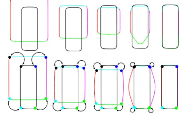
Figure 1. Warping of a rectangle shape into another one. Top row: evolution with E = dW1,2. Bottom row: same energy, with four
provided landmarks, marked by color spots.
6. Experiments
In the experiments showed here, we used the original en-ergy E = dW1,2 and test how our landmark-guided force
modifies the warping and the final matching. Fig. 1 shows the warping of a rectangle into another one. The different parts of the curves are shown with different colors, so that their respective evolution can be followed. The initial warp-ing without any landmark seems natural but it fails discov-ering the matching between the edges of the rectangles, a matching indeed recovered when providing landmarks.
Fig. 2 shows the warping between two hand shapes. The energy E = dW1,2 yields an unnatural warping. Adding
spatially coherent flows makes the warping a bit better but still fails in some parts. With three landmarks only, both a satisfying warping and a good matching are recovered. Fig. 3 shows the warping of a teddy bear into a cartoon char-acter. Without any landmarks, the top row evolution fails matching the ears and arms of the characters. The bottom row shows the evolution with four landmarks. Red spots allow to check a good matching between landmarks.
7. Conclusion
We propose a framework for shape warping based on both shape distances and landmarks. Our method is purely geometric and no extrinsic quantity like a space diffeomor-phism has to be considered. Thanks to recent advances in the level set techniques, a level set implementation is possi-ble, reconciling landmarks and the level set methods. More-over, a matching between shapes is provided at no addi-tional cost. Two- and three-dimensional examples, com-bining shape distance and landmarks, demonstrate the im-provement brought by our approach on both warping and matching, even with a small number of landmarks. Fur-ther work includes investigating for a one-to-one matching between shapes, and a way to cope with other landmarks, such as curves on surfaces in R3.
References
[1] M. Bertalmio, G. Sapiro, L. Cheng, and S. Osher. Varia-tional problems and PDE’s on implicit surfaces. In IEEE, editor, IEEE Workshop on Variational and Level Set Meth-ods, pages 186–193, Vancouver, Canada, July 2001. [2] G. Charpiat, O. Faugeras, and R. Keriven. Approximations
of shape metrics and application to shape warping and em-pirical shape statistics. Foundations of Computational Math-ematics, 5(1):1–58, Feb. 2005.
[3] G. Charpiat, R. Keriven, J. Pons, and O. Faugeras. Design-ing spatially coherent minimizDesign-ing flows for variational prob-lems based on active contours. In 10th International Con-ference on Computer Vision, Beijing, China, 2005.
[4] M. Delfour and J.-P. Zol´esio. Shape analysis via distance functions: Local theory. In Boundaries, interfaces and tran-sitions, volume 13 of CRM Proc. Lecture Notes, pages 91– 123. AMS, Providence, RI, 1998.
[5] A. Dervieux and F. Thomasset. A finite element method for the simulation of Rayleigh-Taylor instability. Lecture Notes in Mathematics, 771:145–159, 1979.
[6] I. Dryden and K. Mardia. Statistical Shape Analysis. John Wiley & Son, 1998.
[7] A. Heyden, G. Sparr, M. Nielsen, and P. Johansen, editors. Proceedings of the 7th European Conference on Computer Vision, Copenhagen, Denmark, May 2002. Springer–Verlag.
[8] D. Kendall. A survey of the statistical theory of shape. Statist. Sci., 4(2):87–120, 1989.
[9] G. Matheron. Random Sets and Integral Geometry. John Wiley & Sons, 1975.
[10] P. Maurel, R. Keriven, and O. Faugeras. Reconciling land-marks and level sets. Technical Report 5726, INRIA, Oct. 2005.
[11] S. Osher and J. Sethian. Fronts propagating with curvature-dependent speed: Algorithms based on Hamilton–Jacobi formulations. Journal of Comp. Physics, 79(1):12–49, 1988. [12] N. Paragios, M. Rousson, and V. Ramesh. Matching distance functions: A shape-to-area variational approach for global-to-local registration. In Heyden et al. [7], pages 775–789. [13] J.-P. Pons, G. Hermosillo, R. Keriven, and O. Faugeras. How
to deal with point correspondences and tangential velocities in the level set framework. In International Conference on Computer Vision, volume 2, pages 894–899, 2003. [14] S. Soatto and A. Yezzi. DEFORMOTION, deforming
mo-tion, shape average and the joint registration and segmenta-tion of images. In Heyden et al. [7], pages 32–47.
Figure 2. Warping of a hand shape into an-other one. Top row: evolution with E= dW1,2.
Middle row: same energy + spatially coherent flows. Bottom row: same energy + spatially coherent flows + three provided landmarks.
Figure 3. Warping of a teddy bear into a car-toon character. Top row: evolution with E = dW1,2. Bottom row, first image: four
land-marks (in blue) provided on the two shapes. Bottom row, remaining images: evolution with E= dW1,2plus the provided landmarks.