HAL Id: hal-02314929
https://hal.archives-ouvertes.fr/hal-02314929
Submitted on 16 Oct 2019
HAL is a multi-disciplinary open access
archive for the deposit and dissemination of
sci-entific research documents, whether they are
pub-lished or not. The documents may come from
teaching and research institutions in France or
abroad, or from public or private research centers.
L’archive ouverte pluridisciplinaire HAL, est
destinée au dépôt et à la diffusion de documents
scientifiques de niveau recherche, publiés ou non,
émanant des établissements d’enseignement et de
recherche français ou étrangers, des laboratoires
publics ou privés.
NDR: Noise and Dimensionality Reduction of CSI for
indoor positioning using deep learning
Abdallah Sobehy, Eric Renault, Paul Muhlethaler
To cite this version:
Abdallah Sobehy, Eric Renault, Paul Muhlethaler. NDR: Noise and Dimensionality Reduction of CSI
for indoor positioning using deep learning. GLOBECOM 2019: IEEE Global Communications
Con-ference, Dec 2019, Waikoloa, HI, United States. pp.1-6, �10.1109/GLOBECOM38437.2019.9013195�.
�hal-02314929�
NDR: Noise and Dimensionality Reduction of CSI for Indoor
Positioning using Deep Learning
Abdallah Sobehy
∗, ´Eric Renault
∗and Paul M¨uhlethaler
†∗Samovar, CNRS, T´el´ecom SudParis, University Paris-Saclay, 9 Rue Charles Fourier, 91000 ´Evry, France †Inria Roquenourt, BP 105, 78153 Le Chesnay Cedex, France
Abstract—Due to the emerging demand for Internet of Things (IoT) applications, indoor positioning has become an invaluable task. We propose NDR, a novel lightweight deep learning solution to the indoor positioning problem. NDR is based on Noise and Dimensionality Reduction of Channel State Information (CSI) of a Multiple-Input Multiple-Output (MIMO) antenna. Based on preliminary data analysis, the magnitude of the CSI is selected as the input feature for a Multilayer Perceptron (MLP) neural network. Polynomial regression is then applied to batches of data points to filter noise and reduce input dimensionality by a factor of 14. The MLP’s hyperparameters are empirically tuned to achieve the highest accuracy. NDR is compared with a state-of-the-art method presented by the authors who designed the MIMO antenna used to generate the dataset. NDR yields a mean error 8 times less than that of its counterpart. We conclude that the arithmetic mean and standard deviation misrepresent the results since the errors follow a log-normal distribution. The mean of the log error distribution of our method translates to a mean error as low as 1.5 cm.
I. INTRODUCTION
The number of mobile and IoT devices is increasing exponentially. It is expected that by 2020, there will be 50 billion connected devices [1]. Consequently, localization services are becoming more and more invaluable for plethora of applications such as autonomous driving, security, routing, etc. The approach to tackle the localization problem depends on multiple factors. These factors include, but are not limited to: the environment, whether indoors or outdoors, used mea-surements such as Global Positioning System (GPS), Received Signal Strength Indication (RSSI) or CSI, and the mobility of nodes. Indoor positioning has been a challenging problem for decades; it is yet to settle on a widely accepted solution that meets both cost and accuracy requirements [2]. One of the challenges in indoor positioning is that it does not have access to GPS service. On the other hand, outdoor positioning has an upper hand due to its access to GPS readings from Line-Of-Sight (LOS) communication. Apart from GPS service, inter-node communication is another source of information to get distance between nodes through RSSI, Time Of Arrival (TOA), or Time Difference Of Arrival (TDOA). The estimated distances are then used to locate nodes in what is known as range-based localization.
With the increasing demand for high throughput data trans-mission, massive MIMO systems are spreading and becoming a viable option to power 5G wireless communication
sys-tems [3]. Information is sent on multiple subcarriers and the Channel State Information (CSI) can be estimated at each sub carrier. The CSI or channel’s frequency response describes the change that occurs to the transmitted signal due to the channel nature, frequency, and antenna’s quality. This kind of richer information has been shown in [4] to be stable with respect to time and robust against environmental changes. Thus, it is a reasonable choice to use CSI for position fingerprinting which maps CSI values to the position of the device.
Without the loss of generality, the proposed solution is described and applied to a dataset provided by the authors of a MIMO channel sounding system [5] where the position of a transmitter is matched to CSI estimated at 924 subcarriers for an 8×2 antenna array. However, the proposed method can be extended to other cases with different properties such as the number of antennas or subcarriers. In order to predict a position based on the 16×924 channel responses, we use an MLP neural network. In Sec. II, we discuss several state-of-the-art methods that tackle the indoor localization problem. In Sec. III, a brief background and the environmental setup are described. Then, the proposed methodology used to process the channel responses along with the chosen structure and hyperparameters of the MLP learning model are presented in Sec. IV. Sec. V includes the experimental results of NDR and a comparison with [5] which is tested on the same dataset. Also, an analysis of the error distribution is presented. Finally, we conclude the presented work and discuss future work in Sec. VI.
II. RELATEDWORK
RSSI is a cost-efficient choice for distance estimation between nodes as it does not require external hardware. However, it has some drawbacks such as its temporal insta-bility. This is due to RSSI’s high sensitivity to environmental changes and various sources of noise such as fading, distor-tion, and multi-path effect [4]. Inter-node distances computed from RSSI are combined to estimate the positions of nodes using methods such as interval analysis [6] or triangulation [7]. As a result of the limitations of RSSI, these solutions are always constrained by its noisy nature. Another solution [8] uses dead reckoning to predict the next position from previous positions. Data fusion is used to combine estimations from different sensor measurements using methods such as Kalman filters [9].
Recently, the fingerprinting trend to achieve high accuracy localization has been steadily moving towards CSI and away
from RSSI [10]. This is due to the richer information content provided by CSI since it is calculated per subcarrier while the RSSI is calculated per packet. Moreover, CSI shows higher temporal stability as opposed to the high variability of RSSI. The FILA solution [11] is one of the very first initiatives to use CSI for localization in complex indoor environments. The CSI of 30 adjacent subcarriers are reduced to CSIef f ective which
is then used in a parametric equation to compute the distance to target node. The parameters of the equation are deduced using a supervised learning method. Finally, using a simple trilateration method [12], the position of the target node is estimated from the computed distances to three anchor nodes. FILA’s closest experimental setup to ours is a 3×4 empty room where it is safe to assume that the received signals were LOS. They attained a mean error less than 0.5 m and they reasonably argued that with the availability of more anchor nodes and with the use of a more accurate trilateration method, the error can be further reduced.
In [5], a 2D Convolutional Neural Network (CNN) is used to localize the transmitter. The dataset used to train and test the CNN is the same set our solution is evaluated with. The authors selected the Re and Im components as input features to their deep learning model. Thus, the input dimension for one position estimation is 16×924×2, which are the numbers of antennas, subcarriers, and complex components respectively. CNNs are able to extract more complex and descriptive higher-level features by processing a window of input features all together [13]. With such high dimensional input along with the use of CNN, the learning and inference processes become more computationally demanding. By se-lecting the magnitude of the CSI as the input feature and using polynomial regression, we are able to reduce the input dimension by a factor of 38 and use a lighter weight MLP neural network and still achieve ≈ 8 times better accuracy. In [4], Intel’s WiFi link 5300 NIC with three antennas and 90 subcarriers per antenna is used for localization. They reached a similar conclusion to use the magnitude of CSI as the input features. They use trained weights between layers in a four-layer MLP as fingerprints to the position of the transmitter. This is achieved through a greedy learning method that trains the weights of one layer at a time based on a stack of Restricted Bolzmann Machines (RBMs) to reduce the complexity [14]. Our method of complexity reduction is based on a simpler process using polynomial regression. It is difficult to compare the estimation error between our method and theirs because of the difference in the number/quality of antennas, environmental noise level, etc. However, the mean error obtained using our proposed method using two antennas and 924 subcarriers is ≈ 6 times less than their mean error which is large enough to have some confidence that our method outperforms theirs. Similar accuracy is achieved using both the magnitude and the phase of CSI fed into the K-nearest neighbours algorithm [15]. K-nearest neighbours algorithm estimates the position by computing a weighted average of k-nearest positions. However, this introduces a complexity due to the need to store the training samples used in the off-line
learning phase which can be a critical memory and processing limitation in some applications.
III. BACKGROUND ANDENVIRONMENTALSETUP
The experimental environment is composed of a transmitter that uses the MIMO channel sounder [5] to transmit sig-nals to an 8×2 antenna array from various positions. The transmissions are orthogonal frequency division multiplexed (OFDM) signals at a radio frequency of 1.25 GHz. The objective is to estimate the transmitter based on the Channel State Information at each subcarrier. Each of the 16 antennas receives the transmission on 1024 subcarriers from which 10% are used as guard bands. Subcarriers have a 20 MHz bandwidth where the modulation scheme of the transmission is Quadrature Phase Shift Keying (QPSK). This leaves 924 estimated complex channel coefficients (real and imaginary components) per antenna that are associated with the position of the transmitter. The estimated frequency response or CSI relates the transmitted signal Ti,j to the received signal Ri,j
at antenna i on subcarrier j as shown in equation (1) where N is the Gaussian white noise.
Ri,j= Ti,j· CSIi,j+ N (1)
CSI is not a scalar but a complex number which can be expressed in polar or cartesian form as depicted in equations (2) and (3) respectively. The available dataset provides the CSI values in cartesian form. Polar form can be computed from cartesian form using equation (4) which is used for the proposed feature selection analysis.
CSIi,j= |M ag|6 φ (2)
CSIi,j = Re + iIm (3)
M ag=pRe2+ Im2
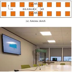
φ= arctan(Re, Im) (4) A tachymeter with a random error below 1 cm is used to estimate the ground truth positions of the transmitter. The antenna array is centered in the local coordinate system at (3.5, -3.15, 1.8). The transmitter is mounted on a vacuum cleaner robot that traverses a 4×2 table which is centered at (4, 0.6, -0.5). Figure (1a) demonstrates a sketch of the antenna array showing its geometry and position in the coordinate system. Figure (1b) shows the indoor environment of the experiment. The distance between the antennas is λ
2 where λ is computed
from the carrier frequency i.e. 1.25 GHz. IV. METHODOLOGY
A. Feature selection
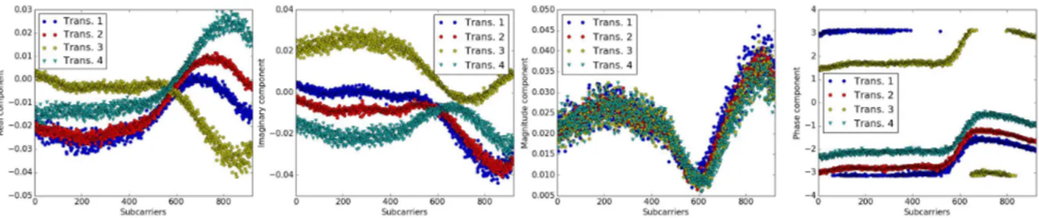
The authors of the antenna [5] chose the real and imaginary components of the estimated channel responses as input features to their learning model. We performed a preliminary analysis on the channel responses by plotting the real and imaginary components as well as the magnitude and phase of
(a) Antenna sketch
(b) Indoor Environment [5]
Fig. 1: Experimental setup
the 924 subcarriers for different transmissions from the same position. Figure 2 shows the responses for four transmissions that occurred from the same position. It can be noted that the magnitude is the most stable component for the same position as opposed to the real, imaginary, or phase components. This phenomenon might be due to the use of a frequency modulation scheme which causes the real, imaginary, and phase components to change in frequency and time while the magnitude changes only with frequency. This conclusion is supported by the statistical analysis performed in [4]. Moreover, using the magnitude as the only feature in the proposed learning model yields the highest accuracy when compared to using any other combinations of the four features. Based on the aforementioned observations, we selected the magnitude of the responses to be the input feature for NDR’s learning model. Consequently, this choice decreases the number of input features by 50% when compared to the choice made in [5] which allows NDR to have a more complex learning model with reasonable processing time.
B. Noise and Dimensionality Reduction through polynomial regression
Even after halving the number of features, the input features are still numerous. The provided data set is composed of≈17k positions with the corresponding 924 subcarrier magnitudes at each of the 16 antennas. For a fair comparison with [5], 90% of the dataset is used to train the model and the rest is used for validation. This results in a 15k × 16 × 924 = 222M input features for the 15k training samples. We introduce a data preprocessing step to further downsize the number of input features by a factor of 14 through polynomial regression.
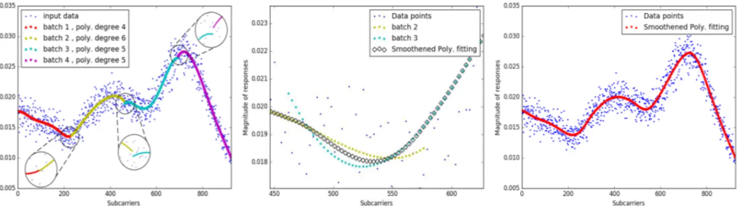
The data points of the magnitudes of the 924 subcarriers are fitted with a line using polynomial regression [16]. The degree of the polynomial is chosen by fitting lines using various degrees, [2,3,4,5,6], then choosing the line that yields the
smallest error when compared to the fitted data. For most cases, a line of a degree 5 or 6 was a reasonable selection. However, it was not always possible to follow some steep curve cases as shown in Fig. 3.
Even with higher degrees, this under-fitting problem per-sisted in some cases. To overcome this limitation, the data points are split into four batches. This number of batches proved adequate for the number and range of subcarrier frequencies. It allows for accurate regression fitting in rea-sonable time and avoids cases such as the one shown in Fig. 3. Polynomial regression is performed on each batch yielding four lines that are concatenated together. This allows to solve the under-fitting problem. However, this introduces some discontinuities that appear at the borders separating adjacent batches as shown in Fig. 4.
To mitigate the discontinuity, the batches are enlarged so that they have a region of intersection where the final esti-mated points in the intersection region are calculated through a weighted averaging method. In the intersection region, the chosen point is a weighted average of the estimation from the two lines fitted to the two adjacent batches. Figure 5 shows a region of intersection between two adjacent batches and the chosen points, shown as black rhombuses. The leftmost point at the intersection region is calculated by giving a weight of 1 to the estimation from the left line, shown in yellow, and a weight of 0 to the estimation from the right line, shown in green. Moving to the right, the weight associated with the estimation from the left line decreases linearly while the weight of the right line increases with the same portion. Finally, at the rightmost point, the chosen point is the estimation from the right line as the weight of the left line is 0. The weighted averaging method allows a smooth transition from the polynomial regression lines from one batch to another. Figure 6 shows the bigger picture where the discontinuity is mitigated.
This data preprocessing step has two critical advantages. First, it mitigates the noise of the estimated magnitudes that can hinder the learning process while conserving the general tendency of change of magnitude over the subcarriers. Second, it allows to use a smaller number of points to describe the magnitude responses. In other words, instead of using all 924 magnitudes on the fitted line, only a subset of magnitudes is used which are equally spaced over the subcarriers spectrum. The size of the subset is chosen empirically by varying the size and choosing a value that hits a sweet spot between di-mensionality reduction and stability of results. Consequently, we chose to describe the magnitude responses with 66 points, decreasing the number of input features by a factor of 14, adding yet another boost to NDR’s time performance. C. Learning Model Structure
We use an MLP to build NDR’s learning model using the tensorflow library [17] because it is lightweight compared to the CNN used in [5]. In order to decide on the structure to be used for the learning model, we varied various hyperparam-eters and chose the values that gives the lowest error on the
Fig. 2: Real, Imaginary, Magnitude and phase components estimated from 4 transmissions at the same position
Fig. 3: Polynomial regression limitations when fitting data points
test set. Table I summarizes the varied hyperparameters and the chosen values that yield the highest accuracy.
TABLE I: Hyperparameters selection.
Hyperparameter Tested values Best found Number of Layers [4,5,6,7,8] 7
Units per Layer [128,256,512,1024,1200] 1024 Epochs [50,100,150,200] 150 Activation Functions [relu, selu, tanh,
softmax]
relu Learning Rate [25 × 10−5, 5 × 10⁻⁴,
1× 10⁻³]
5× 10⁻⁴
Optimizers [Adam, SGD, AdaDelta] Adam L2 Regularization [without,1 × 10−4,
1× 10⁻⁵, 1 × 10⁻⁶]
without L2 Dropout Percentage [1%, 2%, ..., 10%] 3%
V. EXPERIMENTALEVALUATION
The experiments were conducted on a machine using a Linux-based operating system equipped with a 3.8-GHz, 32-GB RAM Intel(R) Xeon(R) quad core CPU E3-1270 v6. The GPU is a 2-GB RAM NVIDIA Quadro K420.
Using the best value for each of the hyperparameters described in Table I, we built an MLP dividing the dataset
into a 90% training set and 10% test set. Using CSI from all 16 antennas, the input dimensions to the MLP is 16×66 for each of the 15k training samples and the output is a 3×1 vector representing the position of the transmitter. The learnt model is then tested against≈ 1.7k samples of the test set. A. 10-fold Cross Validation
We evaluate the performance of NDR with a 10-fold cross validation using all 16 antennas. The average learning time is 1:10 hrs. while the average inference time is 0.1 ms in addition to 22 ms consumed for the polynomial regression step per antenna. It is possible to reduce the polynomial regression time to 8 ms by fixing the polynomial degree instead of attempting several regressions with different de-grees. The mean and standard deviation of estimation errors are computed for each of the 10-fold cross validation runs. The mean estimation error and the standard deviation over all the 10-fold cross validation runs have an average of 0.0445 mand 0.137 m respectively.
Figure 7 shows the error distribution of the test set samples of one of the 10-fold runs. It can be noted that the vast majority of test samples have a very small error with very few outliers that have very large errors. These large errors create a right skew in the distribution of errors. Therefore, the arithmetic mean and standard deviation values misrepresent the nature of the distribution. However, the natural log of errors of the train and test sets approximately follow a normal distribution, as shown in Fig. 8 and 9 respectively. The distribution is more evident in the log error distribution of the training set because the MLP, as expected, performs better on the data used in the learning process. We conclude that the error distribution is log-normal. In such case, the median of errors or the mean and standard deviation of the log of errors are better representatives of the error distribution which we shall use in the following section.In the case where the learning and inference times need to be faster and a slightly larger error can be tolerated, the trade-off between time and accuracy can be compromised by using a less complex MLP. With 100 epochs, 5 layers, and 512 units per layer, the times consumed in learning and inference are 10 mins and 0.06 ms respectively. The mean and standard deviation of errors averaged over the 10-fold runs yielded in this case are 0.0659 m and 0.14 m respectively. For some applications, the given-up accuracy would be considered negligible when compared to the gained performance in time.
Fig. 4: Discontinuity between adjacent batches. Fig. 5: Intersection region between 2 adjacent batches. Fig. 6: Result after discontinuity removal.
Fig. 7: Test set Error distribution.
Fig. 8: Train set Log Error distribution.
B. Varying the Number of Antennas
Authors in [5] chose a 2D CNN to build their deep learning model. With noise and dimensionality reduction achieved in the aforementioned data preprocessing steps, we were able to use a lighter weight neural network, MLP, and still yield higher accuracy. Figure 10 compares the estimation results of NDR with [5] when varying the number of antennas. As expected, using CSI from only two antennas yields the highest mean error because there are fewer training samples. Increasing the number of antennas adds more information which consequently yields better estimations. Using all avail-able information by including data from all 16 antennas, our
Fig. 9: Test set Log Error distribution.
method attains an estimation error which is ≈ 8 times less than the estimation error in [5].
Fig. 10: Comparing our solution using MLP with CNN solution [5]
We have previously shown in Fig. 9, that the errors are fol-lowing a log-normal distribution. Consequently, the arithmetic mean of errors is not the best representative. However, we use it in Fig. 10 for a fair comparison with [5].
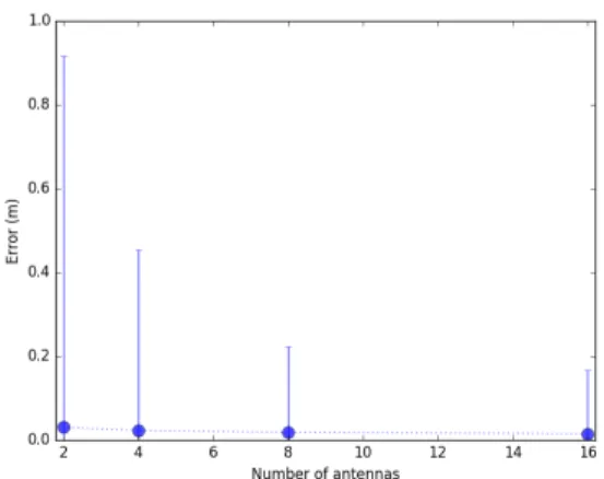
Using the log-normal distribution of errors, we show the estimation error results by plotting the mean and 95th
Fig. 11: Our results showing the 95th
error bars.
Fig. 12: Error Cumulative distribution.
in Fig. 11. Since the error bars are large, the mean values are hardly readable from the figure. The mean values are 0.03 m, 0.023 m, 0.019 m, and 0.015 m when using 2, 4, 8, and 16 antennas respectively. The highly asymmetrical error bars reflect the right skewed nature of the error distribution. Figure 12 shows the cumulative distribution functions of errors when using 2, 4, 8, and 16 antennas respectively. The error values in the x-axis are logarithmically scaled.
VI. CONCLUSION
We presented NDR, a deep learning approach to estimate the position of a transmitter using MIMO channel sounding. NDR entails the choice of the magnitude of channel responses as the input features to the MLP learning model. Noise mitiga-tion and dimensionality reducmitiga-tion are achieved through fitting multiple lines using polynomial regression over four batches of the data points. The fitted lines are then concatenated using a weighted averaging method to remove discontinuity. As a result, the input features for one position are reduced from 16×924×2 as used in [5] to 16×66. Moreover, the chosen subset of points represents the tendency of magnitude change over the subcarriers while mitigating the noise that can hinder the learning process. Thus, we argue that NDR is extensible to other scenarios with different numbers of antennas and
subcarriers. We build a lightweight MLP in comparison to the CNN used in [5] while achieving an error that is 8 times less. We look forward to test our algorithm in other scenarios such as the Non-Line-Of-Sight (NLOS) case. There is a room for improvement in the accuracy through a profound analysis of the outliers and attempting to mitigate them. This can be achieved using data augmentation or ensemble neural network techniques or detailed comparison with NLOS data.
VII. ACKNOWLEDGEMENT
Thanks to the authors of [5] for providing the dataset for the IEEE CTW 2019 Positioning Competition in which NDR achieved the first place. We look forward for further cooperation to be able to test NDR in NLOS scenario. Last but not least, many thanks to Pascal Pernot, Rui Li, Mohamed Badr, and Zahraa Badr for their valuable insights. Special thanks to my wife Enayat Abuismail for her edits and endless support.
REFERENCES
[1] A Nordrum, ”The internet of fewer things [news].” IEEE Spectrum 53, no. 10, 2016. 12-13.
[2] D. Lymberopoulos and J. Liu, ”The microsoft indoor localization competition: Experiences and lessons learned.” IEEE Signal Processing Magazine 34, no. 5, Sept. 2017. 125-140.
[3] F. Boccardi, R. W. Heath Jr., A. Lozano, T. L. Marzetta and P. Popovski, ”Five disruptive technology directions for 5G.” arXiv preprint arXiv:1312.0229, Dec. 2013.
[4] X. Wang, L. Gao, S. Mao and S Pandey, ”DeepFi: Deep learning for indoor fingerprinting using channel state information.” 2015 IEEE wireless communications and networking conference (WCNC), pp. 1666-1671. IEEE, 2015.
[5] M. Arnold, J. Hoydis and S. T. Brink, ”Novel Massive MIMO Channel Sounding Data applied to Deep Learning-based Indoor Positioning.” In SCC 2019; 12th International ITG Conference on Systems, Communi-cations and Coding, pp. 1-6. VDE, 2019.
[6] F. Mourad, H. Snoussi, F. Abdallah, and C. Richard, ”Guaranteed boxed localization in manets by interval analysis and constraints propagation techniques.” In IEEE GLOBECOM 2008-2008 IEEE Global Telecom-munications Conference, pp. 1-5. IEEE, 2008.
[7] A. Sobehy, E. Renault, and P. Muhlethaler, ”Position Certainty Prop-agation: A Localization Service for Ad-Hoc Networks.” Computers 8, no. 1, 2019. 6.
[8] A. Agarwal and S. R. Das, ”Dead reckoning in mobile ad hoc networks.” 2003 IEEE Wireless Communications and Networking, 2003. WCNC 2003., vol. 3, pp. 1838-1843. IEEE, 2003.
[9] W. Kim, M. Park and S. J. Lee, ”Effects of shadow fading in indoor RSSI ranging.” In 2012 14th International Conference on Advanced Communication Technology (ICACT), pp. 1262-1265. IEEE, 2012. [10] J. Xiao, Z. Zhou, Y. Yi and L. M. Ni, ”A survey on wireless indoor
localization from the device perspective.” ACM Computing Surveys (CSUR) 49, no. 2, 2016. 25.
[11] K. Wu, J. Xiao, Y. Yi, M. Gao and L. M. Ni, ”Fila: Fine-grained indoor localization.” In 2012 Proceedings IEEE INFOCOM, pp. 2210-2218. IEEE, 2012.
[12] Y. Liu, Z. Yang, X. Wang and L. Jian, ”Location, localization, and localizability.” Journal of Computer Science and Technology 25, no. 2, 2010. 274-297.
[13] S. Hijazi, R. Kumar and C. Rowen, ”Using convolutional neural networks for image recognition.” Cadence Design Systems Inc.: San Jose, CA, USA, 2015.
[14] Y. Bengio, P. Lamblin, D. Popovici, and H. Larochelle, ”Greedy layer-wise training of deep networks.” In Advances in neural information processing systems, pp. 153-160. 2007.
[15] Y. Chapre, A. Ignjatovic, A. Seneviratne, and S. Jha, ”Csi-mimo: Indoor wi-fi fingerprinting system.” In 39th annual IEEE conference on local computer networks, pp. 202-209. IEEE, 2014.
[16] F. Pedregosa, G. Varoquaux, A. Gramfort, V. Michel, B. Thirion, O. Grisel, M. Blondel et al., ”Scikit-learn: Machine learning in Python.” Journal of machine learning research 12, Oct 2011. 2825-2830. [17] M. Abadi, P. Barham, J. Chen, Z. Chen, A. Davis, J. Dean, M. Devin
et al. ”Tensorflow: A system for large-scale machine learning.” In 12th USENIX Symposium on Operating Systems Design and Implementa-tion (OSDI 16), pp. 265-283. 2016.