ICE MONITORING IN DECEPTION BAY
Progress report 2016-2018
Report submitted to Raglan Mine, a Glencore Company
Attn: Charles Levac
Manager – Risks, Prevention and Environment Rouyn-Noranda (Quebec)
and
Kativik Regional Government Attn: Michael Barrett
Associate Director
Renewable Resources, Environment, Lands and Parks Department
Kuujjuaq (Quebec)
Prepared by
Yves Gauthier, Sophie-Dufour-Beauséjour, Jimmy Poulin, and Monique Bernier, Institut national de la recherche scientifique
Centre Eau Terre Environnement 490, rue de la Couronne Québec (Québec) G1K 9A9
Research Report #1792
For more information, please contact:
Yves Gauthier (Yves.Gauthier@ete.inrs.ca) at 418‐654‐3753
TABLE OF CONTENT
1. Project background and objectives ... 8
2. Project Resources and Collaborative Partners ... 10
3. Summary of achievements and results ... 11
3.1.Instrumentation ... 11
3.1.1.Cameras ... 11
3.1.2.Sonars ... 17
3.2.Field work ... 33
3.2.1.Snow and ice thickness measurements ... 34
3.2.2.Snow and ice roughness measurements... 36
3.2.3.Ice cores and snow pits ... 37
3.3.Satellite imagery ... 44
3.3.1.Historical freeze-up and breakup dates from satellite imagery ... 44
3.3.2.Ice characterization using satellite radar images ... 47
4. Community input and involvement ... 53
4.1.Discussions with land users ... 54
4.2.Activities with the schools ... 54
4.3.Other opportunities for community input ... 55
5. Conclusion and key findings ... 57
6. Phase 4 (2018-2020) ... 60
7. Acknowledgements ... 60
8. References ... 61
APPENDICES ... 62
A. List of Fine Mode RADARSAT-2 images acquired for the project ... 62
LIST OF FIGURES
Figure 1: Location of the study area. ... 8
Figure 2: Freeze-up/Breakup/Freeze-up sequence from November 20 to 26 - Mid-Bay - East view from site #2 looking at Moosehead Island (Reconyx camera). ... 13
Figure 3: Breakup from June 22-26, 2016. Top: West view at the mouth of Deception Bay (from Black Point Reconyx camera); Bottom: North view of Arctic Island (from Black Point Spypoint Camera). ... 13
Figure 4: Thermal freeze-up in the southern part of the bay... 14
Figure 5: Dynamic freeze-up in the northern part of the bay ... 14
Figure 6 : 2017 breakup from June 5 to 8 – Bottom end of the bay – South and East view (from site #3 Panasonic camera. ... 15
Figure 7 Breakup on June 10, 2017, near Moosehead Island - east view from site #2 Reconyx camera). ... 15
Figure 8: Bathymetry of Deception Bay and location of cameras (with field of view)... 16
Figure 9 : Freeze-up and breakup sequences (colors) compared to air temperatures (line). ... 17
Figure 10: Location of SWIP and IPS deployments for 2015-2016 and 2016-2017 ... 18
Figure 11: Deployment of the IPS (with anchor) from a boat in Deception Bay ... 18
Figure 12 : Ice thickness vs time from the 2015-2016 SWIP data. ... 21
Figure 13: Ice thickness vs time from SWIP data during the 2015 freeze-up. ... 22
Figure 14: Freeze-up above the SWIP in November 2015. Left: West view from site #3 (Panasonic camera). Right: East view from site #2 (Reconyx camera). ... 23
Figure 15: Ice thickness vs time from SWIP data during the 2016 breakup... 24
Figure 16: Breakup above the SWIP in June 2016. West view from site #3 (Panasonic camera). 25 Figure 17: Ice thickness vs time from 2016-2017 SWIP data. ... 26
Figure 18: Ice thickness vs time from SWIP data during the 2016 freeze-up ... 27
Figure 19: Freeze-up above the SWIP in December 2016. East view from site #2 (Reconyx camera). ... 27
Figure 20: Ice thickness vs time from SWIP data during the 2017 breakup... 28
Figure 21: Break-up above the SWIP in June 2017. ... 28
Figure 22: Ice thickness vs time from 2016-2017 IPS data.. ... 29
Figure 23: Ice thickness vs time from IPS data during the 2016 freeze-up. ... 30
Figure 25: The MV Arctic maneuvering to leave the bay. ... 30 Figure 26: Ice thickness vs time from IPS data during the 2017 breakup. ... 31 Figure 27: Breakup above the IPS in June 2017. North-east view from site #3 (Panasonic camera). ... 32 Figure 28: Ice thickness vs time from IPS data in January 2017. Transits of MVs Arctic and Nunavik in Deception Bay are identified. ... 33 Figure 29 : Location of sampling points in Deception Bay. ... 34 Figure 30 : Snow (a-b) and ice (c-d) thicknesses measured in Salluit, Deception Bay and Kangiqsujuaq in 2016 and 2017. Markers = mean; Error bars = standard deviation. Empty markers indicate sparse measurements. Also shown is the best linear fit to the data, with their associated parameters. ... 35 Figure 31 : Deviation from mean snow (left) and mean ice (right) thicknesses for each sampling point in Salluit in April 2017. ... 36 Figure 32 : Deviation from the mean ice thickness for each sampling point in Deception Bay in April 2017, in relation to bathymetry. ... 36 Figure 33 : Snow and ice surface roughness observations in Wakeham Bay in January 2018. .... 37 Figure 34 : Ice cores extracted and sliced (featured: Juupi Tuniq, Pierre-Olivier Carreau, Markusi Jaaka). ... 39 Figure 35 : Ice core slices prepared for salinity measurements (featured: Sophie Dufour-Beauséjour). ... 39 Figure 36 : Ice cores extracted and prepared for CT-Scan. ... 40 Figure 37 : CT-scan density data products (2D-grey levels and 3D-blue) for two samples. First sample (a-b) shows air bubbles at the top while second sample (c-d) shows vertical brine channels. ... 40 Figure 38 : Example of density and porosity measurements for an ice core sample of Deception Bay in January 2016. ... 40 Figure 39 : Vertical salinity profiles of first-year ice from November to April, reproduced from Weeks and Ackley, 1982. ... 41 Figure 40: Salinity profiles for ice cores extracted in Deception Bay in January (blue line) and April (black line) 2017. ... 42 Figure 41 : Snow (black) and first 30cm of ice (blue) salinity profiles in Deception Bay in January 2018. ... 42 Figure 42 : CT-scans and salinity measurements of ice cores taken over the SWIP in Deception Bay in January and April 2017. ... 43 Figure 43 : Evolution of the estimated breakup date in Deception Bay over the last 30 years from satellite images. The dotted lines between 2002-2016 represent the breakup date estimated from the ice concentration maps produced by the Canadian Ice Service every one or two weeks at a coarser resolution. ... 45
Figure 44 : Evolution of the estimated breakup date in Salluit and Kangiqsujuaq over the last 30 years from satellite images. The dotted lines between 2002-2016 represent the breakup date estimated from the ice concentration maps produced by the Canadian Ice Service every one or two weeks at a coarser resolution. ... 46 Figure 45 : Evolution of the estimated freeze-up date in Deception Bay in the recent years from satellite images. The dotted lines between represent the breakup date estimated from the ice concentration maps produced by the Canadian Ice Service every one or two weeks at a coarser resolution. ... 46 Figure 46 : Evolution of the estimated freeze-up date in Salluit and Kangiqsujuaq over the recent years from satellite images. The dotted lines represent the breakup date estimated from the ice concentration maps produced by the Canadian Ice Service every one or two weeks at a coarser resolution. ... 47 Figure 47 : Radar images processing routine ... 48 Figure 48 : RADARSAT-2 and TerraSAR-X images acquired over Deception Bay in December 2015 and associated K-means clustering result. ... 50 Figure 49 : Multi-temporal classification results for the 2015-2016 ice season in Deception Bay using 5 RADARSAT-2 images (left) and 11 TerraSAR-X images (right). ... 51 Figure 50 : TerraSAR-X image acquired on December 24th 2015 over Deception Bay. RGB composite: K1, K0, K5. Polygons delimit areas of interest for ship track digitizing. Polylines correspond to all tracks digitized on this image. Wharfs for Glencore (blue) and Canadian Royalties (red) are also shown. ... 52 Figure 51 : RGB representation (HH, HV, VV) of RADARSAT-2 images acquired over Kangiqsujuaq (January 10th) and Salluit (January 30th) in 2017. Ice thickness is shown in boxes. The green boxes correspond to observations of rough ice. ... 53 Figure 52: Ice monitoring project booth at the Raglan Mine Environmental Forum in Kangiqsujuaq in October 2017. ... 54
LIST OF TABLES
Table 1 : Project resources and research partners ... 10
Table 2: Instrument installation and maintenance and data recovery visits ... 11
Table 3: Summary of the 2015-2016 ice cover season... 12
Table 4 : Summary of the 2016-2017 ice cover season ... 14
Table 5: Icebreakers transit in the bay during the 2016-2017 ice season (Blue cells = open water; White cells = ice cover). ... 32
Table 6: Field campaigns schedule ... 33
Table 7 : Mean snow and ice thickness measured in January 2018. ... 35
Table 8: Sources of images used for historical freeze-up and breakup analysis ... 44
Table 9 : Characteristics of RADARSAT-2 and TerraSAR-X satellites ... 47
Table 10: Outreach activities done at Arsaniq and Ikusik High Schools in Salluit and Kangiqsujuaq since the beginning of the project ... 56
1. Project background and objectives
The project “Ice monitoring in Deception Bay” was initiated in 2015 through a technical and administrative agreement between the Kativik Regional Government (KRG) and Raglan Mine, a Glencore company. INRS acted as a consultant to KRG and as a partner to the project. The work was also funded over 2015-2018 by Polar Knowledge Canada, as a component of the Safe Passage Project (Leader: University of Victoria). INRS is an institution partner of the Safe Passage project and is responsible for the Deception Bay Component, under the leadership of Professor Monique Bernier.
The global objective of the Deception Bay project is to better understand the interactions between the ice cover of, changing climate, winter navigation, safe access to the territory for Inuit communities and protection of the bay’s ecosystem. The specific objective of this agreement is to assess various monitoring techniques to document the characteristics, processes and variability of the ice cover during three winter seasons (2015-2018). Three phases were planned: 1) Characterization (2015); 2) Instrumentation (2015-2016); and 3) Data acquisition, analysis and dissemination (2015-2018). Phase 3 also included instrument maintenance and data recovering. Methodology involved on-site sensors, field measurements, satellites images and community involvement. Control observations and measurements are acquired in the neighboring communities of Salluit and Kangiqsujuaq (Figure 1).
The service contract between KRG and INRS ended in July 2016 (Phases 1 and 2). INRS submitted a final report (Gauthier et al, 2016, http://espace.inrs.ca/4846/1/R1679.pdf) to KRG in June 2016 concerning the period of contract (2015-2016) and combining:
1. Visit report (Deception Bay, Salluit, Kangiqsujuaq)
2. Site characterization report (including the instruments installation plan and the satellite images acquisition plan
3. Installation report for the cameras and the echo-sounders, the data archival and dissemination plan.
4. Field work report.
However, through the funding by Polar Knowledge Canada (Safe Passage project), the in kind and financial contribution by KRG and the in kind contribution by Raglan Mine (a Glencore company), the project continued over 2016-2017 and 2017-2018.
The present report is a summary report covering the activities conducted between July 2016
and March 2018 (Phase 3). The full spectrum of data and analysis is reserved for scientific
publications that are in preparation or planned over the next year. The drafts of those publications will be sent to Raglan Mine for release approval when available.
2. Project Resources and Collaborative Partners
Table 1 lists the people involved in the project.
Table 1: Project resources and research partners
INRS INUIT COLLABORATORS
Dr Monique Bernier (professor) Salluit : Kangiqsujuaq:
Yves Gauthier (Research professional) Juupi Tuniq Noah Annahatak Jimmy Poulin (Research professional) Markusi Jaaka Peter Arngak Sophie Dufour-Beauséjour (PhD student) Pierre Lebreux Elijah Ningiuruvik Pierre-Olivier Carreau (Undergrad intern) Charlie Ikey Maasiu Arngak Étienne Lauzier-Hudon (Undergrad intern) Johnny Ashevak Elijah Qisiiq Charles-Éric Noël Laflamme (Undergrad intern) Joannasie Kakayuk Charlie Alaku Charles Paradis (Undergrad intern) Kululak Tayara Joe Pilurtuut Valérie Plante Lévesque (PhD student) Adamie Raly Kadjulik Adamie Jr. Sakiagak
Putulik Cameron Dany Alaku
KRG (Kativik Regional Government) Michael Cameron Jamie Jaaka Véronique Gilbert (Environmental specialist) Chris Alaku
Michael Barrett (Assistant director) Denis Napartuk
Raglan Mine, a Glencore company Jani Kenuajuak Charles Levac (Manager – Risks, Prevention and Environment) Luuku Isaac Amélie Rouleau (Director - Public Affaires, Communications and
Community Engagement)
Jimmy Kakayuk Frédéric Lapointe (Superintendent - Environment) Casey Mark Mélanie Côté (Superintendent - Environment) Eyetsiaq Papigatuk
CIS (Canadian Ice Service)
Tom Zagon (Physical scientist)
FEDNAV
Pascal Bourbonnais (Ice analyst)
ASL Environmental Sciences Inc.
Ed Ross (Project Manager)
DLR
3. Summary of achievements and results
3.1. Instrumentation
A summary of all instrument related missions in Deception Bay are listed inTable 2. These installation and maintenance missions were done by INRS, KRG and local Inuit collaborators.
Table 2: Instrument installation and maintenance and data recovery visits
Dates Installation Maintenance Data recovery
September 10-11, 2015 Camera network -
-October 29, 2015 SWIP -
-September 15-19, 2016 IPS Camera network SWIP
Camera network SWIP September 15-19, 2017 - Camera network
IPS
Camera network IPS October 13-16, 2017 - Camera network
SWIP SWIP
3.1.1. Cameras
In September 2016, the photos were downloaded from the memory cards of the cameras and systems were checked. The inspection revealed that data acquisition at site #2 had been cut short because the solar panel was teared down in December 2016. In September 2017, the photos were downloaded from the memory cards of the cameras and systems were checked. At site #1 (Black Point), the system had stopped one week after the 2016 maintenance visit due to the wires overheating. At site #2 (West bank), the inspection revealed that the solar panel reinstalled in winter 2017 had malfunctioned. Cameras on site #2 ran throughout the season using their batteries, but no pictures from site #1 are available for this season. After repairs, the systems were relaunched in October 2017. Over 60 000 photos of the ice cover (Table 2) were taken during the first two years of the project. Data from 2017-2018 will be retrieved in September 2018. These pictures were taken hourly from different locations on both shores of the bay.
Using this database, a detailed timeline of freeze-up and breakup in Deception Bay was established for the first two years of the project. From the analysis of all available photos, the sequence of the 2015-2016 ice cover season was established (Table 3). Figure 2 shows the 2015 fall freeze-up sequence from November 20 to 26 - Mid-Bay. Figure 3 shows the breakup sequence at the mouth of the bay that same year.
Table 2: Data recovered from the camera network for 2015-2017 Reconyx camera Site #1 Black Point Looking West Spypoint Camera Site #1 Black Point Looking North Reconyx Camera Site #2 West bank Looking East Browning Camera Site #2 West bank Looking North Panasonic Real-Time Camera Site #3 Raglan Infrastructure 4 views/hr Period of acquisition 2015-2016 2015-09-11 2016-09-16 2015-09-15 2016-09-16 2015-09-11 2016-01-27 2015-09-11 2016-01-17 2015-09-11 2016-09-16 Number of photos 2015-2016 4210 4226 1323 952 18 518 Period of acquisition 2016-2017 - - 2016-09-18 2017-09-16 2016-09-18 2017-05-06 2016-09-17 2017-09-15 Number of photos 2016-2017 - - 8368 4109 18 458
Table 3: Summary of the 2015-2016 ice cover season
First appearance of ice Final complete ice cover First appearance of water First water free of ice Last ice observation Ice duration* (days) Mouth of the bay October 29, 2015 November 26, 2015 June 22, 2016 June 26, 2016 July 2, 2016 213 Middle of the bay October 29, 2015 November 24, 2015 June 21, 2016 June 23, 2016 June 29, 2016 212 Bottom end of the bay October 27, 2015 November 11, 2015 June 18, 2016 June 21, 2016 June 28, 2016 223
*Ice duration is the number of days between the final complete ice cover and the first day of water free of ice.
The first floating ice pieces were spotted at the end of October 2015. Then a complete freeze-up was observed in the bay at mid-November. However, warmer temperatures and extreme winds on November 17 to 21 melted the snow cover and dismantled the ice cover from mid-bay onward (Figure 2), leaving the ice intact in the bottom end of the bay. A complete ice cover formed again a few days later and stayed in place throughout the winter.
Figure 2: Freeze-up/Breakup/Freeze-up sequence from November 20 to 26 - Mid-Bay - East view from site #2 looking at Moosehead Island (Reconyx camera).
The 2016 spring breakup was quick (Figure 3). It started at the bottom end of the bay on June 18, 2016 and progressed towards the mouth. There were eight days between the first open water lead and the complete dismantlement of the ice cover in the bay. However, floating ice pieces were spotted regularly until early July.
Figure 3: Breakup from June 22-26, 2016. Top: West view at the mouth of Deception Bay (from Black Point Reconyx camera); Bottom: North view of Arctic Island (from Black Point Spypoint Camera).
The same analysis was done over the 2016-2017 season (Table 4), without photos from Black Point. The information for the mouth of the bay comes from the far view of the Panasonic camera.
Table 4: Summary of the 2016-2017 ice cover season
First appearance of
ice
Final complete ice cover First appearance of water First water free of ice Last ice observation Ice duration (days) Mouth of the
bay - December 9, 2016 June 12, 2017
June 19, 2017 - 192 Middle of the bay November 21, 2016 December 7, 2016 June 10, 2017 June 14, 2017 June 21, 2017 190 Bottom end of the bay November 10, 2016 November 28, 2016 June 5, 2017 June 9, 2017 June 15, 2017 193 The first appearance of slush ice in the bay came in the second week of November 2016. A thermal freeze-up started in the southern part of the bay on November 28 (Figure 4). Farther out, from Moosehead Island to the mouth of the bay, ice floated in from the strait on December 5 and consolidated up to December 7 (Figure 5). The mouth of the bay was completely frozen on December 9, 2016.
Figure 4: Thermal freeze-up in the southern part of the bay
The 2017 breakup occurred from south to north, in a similar sequence to 2016. Open water was first observed on June 5, 2017 near the outlet of Deception Bay. It progressed towards Moosehead Island on June 10 and reached the mouth of the bay a few days later (Figure 6 and Figure 7).
Figure 6: 2017 breakup from June 5 to 8 – Bottom end of the bay – South and East view from site #3 (Panasonic camera).
Figure 7:Breakup on June 10, 2017, near Moosehead Island - East view from site #2 (Reconyx camera).
Differences in ice duration between the two seasons depend on the region of the bay observed. In the middle of the bay, the ice season was three weeks shorter in 2016-2017 than in 2015-2016. For the bottom of the bay, the difference is 30 days.
We can also observe different freeze-up patterns south and north of Moosehead Island. The south part is deeper and more protected with better chances of a thermal freeze-up. The north part seems more exposed to the extreme conditions and freeze-up is dynamic, with ice being
brought in from the Hudson Strait. The breakup sequence for the two years observed seems constant, with open water leads starting at the bottom end of the bay and progressing steadily towards the strait.
The ice dynamic appears to be closely related to bathymetry. From the camera at site #2 (looking at Moosehead Island), the ice forms first on the east side of the bay. See for example Figure 2 and Figure 5. This corresponds to the shallowest part of the bay (Figure 8). It is also the last section to break up (Figure 7).
Figure 8: Bathymetry of Deception Bay and location of cameras (with field of view)
The observed ice freeze-up and breakup timelines were matched with the air temperatures time-series extracted from the cameras’ temperature measurements. Figure 9 shows the air temperature from the cameras at the mouth of Deception Bay compared to the ice sequences. It takes three to five weeks of freezing air (<0°C) temperatures before ice is first observed. It then takes another 2 to 3 weeks for the ice cover to be complete and permanent. In spring, it takes 4 to 6 weeks of air temperature above 0°C before breakup starts. At this point, it only takes a few days for the ice cover to be cleared away for the first time. Here we do not show the subsequent period where ice debris come and go in the bay with tides, winds and currents.
Figure 9: Freeze-up and breakup sequences (colors) compared to air temperatures (line).
3.1.2. Sonars
The Shallow Water Ice Profiler (SWIP) and the Ice Profiling Sonar (IPS) are upward-looking sonar devices mounted on the ocean floor that measure ice draft, from which we can derive ice thicknesses at a very high temporal resolution.
The SWIP was first installed in Deception Bay (near Moosehead Island) in October 2015 (Figure 9) and retrieved by divers in September 2016 to download data and change the battery. The system was then redeployed by the divers. The same actions were performed in October 2017. The Ice Profiling Sonar (IPS) and its acoustic release device were deployed in deep water (Figure 10 and Figure 11) in September 2016. It was retrieved in September 2017, at which point data was downloaded, batteries were changed and the instrument was redeployed. Both instruments were described in the previous report (Gauthier et al, 2016).
Figure 10: Location of SWIP and IPS deployments for 2015-2016 and 2016-2017
Figure 11: Deployment of the IPS (with anchor) from a boat in Deception Bay (2016)
Several processing steps are necessary to go from the raw signal of the instruments to the ice thickness measurements. Several factors may impair the precision of the instrument and the ice thickness results.
Theory
When the SWIP is deployed, the acoustic transducer transmits pulses of a predefined duration and time interval. For the 2015-2016 measurements, the SWIP emitted a 68 µs pulse every
second. This acoustic pulse travels towards the surface as a conical beam. Part is absorbed by the medium and part is lost in the air. However, part is reflected back to the SWIP. The air-water interface, an ice cover, air bubbles in the water, plankton, or suspended frazil ice are all potential causes for such reflection. The SWIP measures the amplitude and persistence of the echo, as well as the time delay,𝑇, between the emitted and reflected signal. The distance 𝑅 between the SWIP and the element at the source of the echo can be determined knowing the sound speed c in water:
R =Tc
2 [1]
Equation 1 assumes that:
- the speed of sound is constant (isothermal water column);
- there has been only one back and forth travel of the signal between the SWIP and the reflecting element;
- 𝑅 is vertical (which is not always the case).
The SWIP can capture up to five echoes from various sources for each pulse. A decision algorithm based on amplitude, persistence and distance is used to determine which echoes are from the relevant target here (air-water interface and ice cover). To do that, some specific parameters are set up by the user (min and max distance, thresholds for detecting a reflector, minimal persistence of the echo).
In order to estimate the ice draft, the SWIP also measures the sensor tilt, the water pressure and the water temperature. By subtracting the water pressure at the SWIP, 𝑃𝐵𝑇𝑀, from the
atmospheric pressure in the area, PATM, we can calculate the height of the water column above
the SWIP:
η = (PBTM− PATM
ρg ) − ΔD [2]
ρ is the water density, g is the gravitational constant and ΔD is the effective distance between the pressure sensor and the acoustic transducer.
Subtracting R from η should give us the ice draft. However, R was supposed vertical. It has to be corrected using data from the tilt sensor. And the speed of sound used in eq.1 was an approximation. It changes with water temperature and salinity, which may be heterogeneous
along the water column. A correction factor 𝛽 is calculated based on data from the temperature sensor. Therefore, ice draft (d) is obtained with:
d = η − R β cos θ [3]
Finally, supposing constant isostatic equilibrium, ice draft (d) is converted to ice thickness 𝑇𝐼
based on the Archimedes principle (the weight of ice and snow should equal the weight of displaced water) with:
TI=
ρWd − TSρS ρI
[4]
where:
ρW is the water density, ρS is the snow density, ρI, is the ice density and TS is the snow
thickness.
Data processing
Sonar data is processed using the IPS5Extract software from ASL Environmental Sciences. After the data is downloaded from the instrument, pre-processing is necessary to mask outliers caused by the electronic instruments, reduce the noise in the time-series and interpolate over missing data points. Only low tide data is used for the SWIP because the pressure sensor saturates at high tide. Atmospheric pressure data from the weather station in Salluit (50 km away) was used for the ice thickness computation, as there is no weather station in Deception Bay. This may cause some errors in the ice thickness data series if there are discrepancies between the weather in Salluit and in Deception Bay, for instance where there is a storm at one of the sites. To avoid this issue in the future, a barometer was installed in Deception Bay in September 2017.
After this pre-processing, the ice draft and ice thickness were calculated from equations 1 to 4. The water column height above the sonar is (eq. 2) is computed using the water density, which is estimated from water temperature measurements and water salinity values taken from the literature on Deception Bay. A preliminary ice draft is obtained from equation 3, first considering the β correction factor equal to 1. The correction curve is then calculated from ice thickness measurements taken above the SWIP during winter and other considerations on the
speed of sound and the water density. The final ice draft data series is computed using this beta curve. Some smoothing and downsampling may be done on the resulting series to reduce the density of the data.
Ice thickness is computed from the ice draft (eq. 4) using snow and ice densities estimated from the literature and the snow thickness measured on the field.
Results SWIP 2015-2016
The ice thickness computed from 2015-2016 SWIP data is presented in Figure 12 for the whole season and compared to values measured on the field. The black dot is the mean ice thickness and the green vertical line is the range of values from all drillings in the bay at that period (south of Moosehead Island). Overall, the field data seem to confirm the general adequacy of the ice thickness calculated from the SWIP. But we need to further validate the results by looking at the data in more details.
Figure 12: Ice thickness vs time from the 2015-2016 SWIP data.
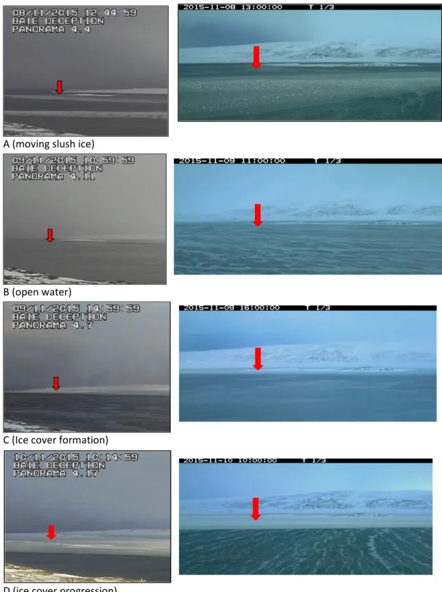
Freeze-up period: The graph in Figure 13 indicates that the ice cover formed above the SWIP on
November 9, 2015. The photo sequence of Figure 14 confirms the timing of ice formation. The ice thickness cannot be validated at freeze-up for lack of field measurements in November.
Figure 13: Ice thickness vs time from SWIP data during the 2015 freeze-up.
However, the decrease in ice thickness values observed between November 16 and November 20 on Figure 13 corresponds to a period of extreme weather, which may have an impact on the accuracy of the atmospheric pressure values used for Deception Bay. Above 0°C air temperatures were measured from November 18 to 21 and winds over 100 km/h were measured on November 17 to 20 at the Salluit weather station. This would indicate that at these times, the atmospheric pressure (PATM) in Deception Bay could be different from the one
measured in Salluit, potentially provoking underestimation of the water levels (η) over the SWIP. A difference of 3 kPa can lead to a difference of 30cm on the ice draft estimate. Near the mooring, but not directly above it, the snow on the ice had completely melted on November 20 and a large part of the ice cover in Deception Bay broke off on November 21 and 22 (Figure 2). The ice cover seems to have been stable over the mooring however and no observations from the camera pictures can explain the decrease in ice thickness as measured by the SWIP.
Several times during the season, the SWIP data showed a significant decrease of the ice draft or thickness while photos showed stable conditions at the surface. On these same occasions however, we could observe rain or snow on the camera photos. The influence of weather events on the ice thickness data series computed from sonar measurements needs to be investigated more thoroughly.
A (moving slush ice)
B (open water)
C (Ice cover formation)
D (ice cover progression)
Figure 14: Freeze-up above the SWIP in November 2015. Left: West view from site #3 (Panasonic camera). Right: East view from site #2 (Reconyx camera).
Breakup period: Figure 15 shows the SWIP measurements during the breakup period of 2016.
The last days of the ice cover would be during the last week of June 2016. The photos sequence of Figure 16 clearly shows the end of the ice cover over the SWIP mooring between June 22 and June 23.
Figure 15: Ice thickness vs time from SWIP data during the 2016 breakup
From this analysis, we can determine that the SWIP measurements provide a good assessment of the ice thickness evolution during the season. The timing of the freeze-up and breakup over the SWIP mooring are well detected and the estimated ice thicknesses are within the range of measured thicknesses during field visits. However, results have to be interpreted with caution and by using complementary sources of information because there are still many sources of uncertainties that can affect the quality of the results.
A (ice cover decaying)
B (open water)
C (open water)
Results SWIP 2016-2017
The same analysis was performed on the 2016-2017 SWIP data. The ice thickness estimates match the field measurements of January and April 2017 (Figure 17). There is a residual sinusoidal noise in the 2016-2017 data series which is caused by the tides and has not yet been completely removed.
Figure 17: Ice thickness vs time from 2016-2017 SWIP data.
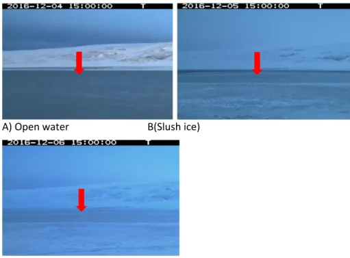
Freeze-up period: The freeze-up dynamics are also well-detected. Numerous episodes of drifting
ice floes were observed in November 2016. The frequency of such events increased in the first week of December and freeze-up occurred over the mooring between December 5 and 6, 2016 (Figure 18 and Figure 19).
Figure 18: Ice thickness vs time from SWIP data during the 2016 freeze-up
A) Open water B(Slush ice)
C) Ice cover
Breakup period: The SWIP data indicates breakup on June 11, 2017 (Figure 20), with drifting
floes on June 14. This is confirmed by the photos at site #2 (Figure 21).
Figure 20: Ice thickness vs time from SWIP data during the 2017 breakup.
A (ice cover decaying) B (ice cover decaying)
C (Open water) D) Passing floes
Results IPS 2016-2017
The IPS was first retrieved in September 2017. The instrument is located under the ships’ track (Figure 10), in the area where the ships usually maneuver after backing out of the dock. The 2016-2017 data were processed with the same approach as for the SWIP data. Preliminary results of the ice thickness seasonal evolution estimated from the IPS are presented in Figure 22. The average ice thickness values match the field measurements, although the time-series is dominated by major events in ice thickness amplitude which will be discussed later.
Figure 22: Ice thickness vs time from 2016-2017 IPS data..
Freeze-up period: Freeze-up over the IPS is detected on November 27 from the sonar data
(Figure 23), which is corroborated by the picture shown in Figure 24. The MV Arctic arrived in the bay on the morning of November 27, just a couple of hours before freeze-up. The ship left on December 9 (Figure 25), having a small effect on the IPS signal. The MV Nunavik came in on November 17 and left in the night of the 26th, before freeze-up.
Figure 23: Ice thickness vs time from IPS data during the 2016 freeze-up.
Figure 24: First appearance of ice above IPS mooring in November 2016.
Breakup period: The IPS data indicates that breakup occurred between June 2 and 8, 2017
(Figure 26). The photo sequence from Figure 27 shows an open water lead approaching from the north towards the IPS area on June 2, followed by an episode of freezing rain and a stabilization of the ice cover. The MV Arctic came in the bay on June 5th. Breakup seems to have reached the area over the IPS on June 7 and 8, leaving the water free of ice on the 9th.
Figure 26: Ice thickness vs time from IPS data during the 2017 breakup.
Overall, SWIP measurements indicate an ice duration of 227 days in 2015-2016 and only 187 days in 2016-2017, with a maximum ice thickness of over 150 cm in 2015-2016 compared to only 110 cm in 2016-2017. Data from the IPS (2016-2017) yields similar results, with a maximum ice thickness of roughly 110 cm and an ice duration of 194 days.
Figure 27: Breakup above the IPS in June 2017. North-east view from site #3 (Panasonic camera).
Ship’s passage: Several sudden shifts in the ice thickness measurements can be observed in the
IPS data (Figure 28). Icebreaker transit dates for the 2016-2017 ice season are listed in Table 5. Figure 28 shows that changes in the ice thickness measured by the IPS can be correlated with icebreakers passing over the sonar. The impact of the ship’s passage on the ice cover directly above the IPS depends on the position of the ship relative to the sonar during its transit.
Table 5: Icebreakers transit in the bay during the 2016-2017 ice season (Blue cells = open water; White cells = ice cover).
2016-2017 In Out In Out In Out In Out
Arctic
(Raglan) Nov.27 Dec.9 Jan.9 Jan.23 Mar.6 Mar.15 Jun.5 Jun.15
Nunavik
Figure 28: Ice thickness vs time from IPS data in January 2017. Transits of MVs Arctic and Nunavik in Deception Bay are identified.
3.2. Field work
Field campaigns were conducted in each bay twice every year (Table 6), to collect data on the characteristics of the ice cover (ice vertical structure, ice thickness, ice salinity profile, snow thickness). Ice drilling and ice coring were performed. Overall, 5 campaigns were done. The next campaign is scheduled for early May 2018.
Table 6: Field campaigns schedule
Field campaign #1 2016 Field campaign #2 2016 Field campaign #3 2017 Field campaign #4 2017 Field campaign #5 2018 Measurements by Inuit collaborators only Site
Jan 23-24 Apr 18-20 Jan 10 Apr 25 Jan 27-28 Mar 14, 2016 Feb 14, 2017 Apr 6, 2017 Kangiqsujuaq (Wakeham Bay) Jan 25-26 Apr 21-22 (cancelled)
Jan 18 Apr 27 Jan 30 Feb 5, 2016 Jan 26, 2017 Mar 21, 2017
Salluit (Salluit Fjord) Jan. 20-22 Apr 23-25 Jan 13-14 Apr 28-29 Feb 1-2 Feb 12 and 26, 2016
Mar 18, 2016 Jan 29, 2017
3.2.1. Snow and ice thickness measurements
In each bay, over 20 to 25 georeferenced sampling points are revisited (Figure 29).
Figure 29 : Location of sampling points in Deception Bay.
At each sampling point, the snow thickness is measured in centimeters using a ruler. A two-inches wide hole is then drilled in the ice cover using a Kovacs ice drill. Through this hole, the ice thickness is measured in centimeters using a Kovacs ice measuring tape.
Figure 30 shows the mean snow and ice thickness measurements for the 2016 and 2017 field campaigns. In winter 2016, as there is more snow on average in Kangiqsujuaq (Graph a), the ice cover was thicker in Deception Bay (Graph c). In 2017, Salluit shows the thinnest snow cover (graph b) and the thickest ice cover (Graph d). The estimated ice growth rate was about 0.5 cm/day in 2016 for all bays, but the larger differences in snow depth at the end of winter 2017 would create differences in the estimated ice growth rate as well (between 0.3 and 0.6 cm/day).
Figure 30: Snow (a-b) and ice (c-d) thicknesses measured in Salluit, Deception Bay and Kangiqsujuaq in 2016 and 2017. Markers = mean; Error bars = standard deviation. Empty markers indicate sparse measurements. Also shown is the best linear fit to the data, with their associated parameters.
Measurements from January 27 to February 2, 2018 are presented in Table 7.
Table 7: Mean snow and ice thickness measured in January 2018.
Site Mean snow thickness Mean ice thickness
Salluit 6 cm 81 cm
Deception Bay 8 cm 83 cm
Kangiqsujuaq 8 cm 71 cm
The close relationship between snow depth and ice thickness can also be observed from their respective spatial distribution. For example, Figure 31 shows the deviation from the mean snow or ice thickness for each sampling point in Salluit in April 2017. In general, areas with a thinner snow cover (red) also have a thicker ice cover (blue). This is observed for each bay, which highlights the importance of understanding the factors determining snow accumulation patterns such as dominating winds and mountains.
Apart from the presence of a snow cover, another parameter which influences the ice thickness is water depth. Figure 32 shows that in Deception Bay (April 2017), thicker ice is found over the deep main channel while thinner ice is observed around Moosehead Island.
Figure 31: Deviation from mean snow (left) and mean ice (right) thicknesses for each sampling point in Salluit in April 2017.
Figure 32: Deviation from the mean ice thickness for each sampling point in Deception Bay in April 2017, in relation to bathymetry.
3.2.2. Snow and ice roughness measurements
The surface roughness of the snow-covered sea ice has an influence on the satellite radar observations of the ice and may also have an impact on snow-mobile transport. Also, areas of broken sea ice caused by the wind and currents may be harder to travel on when there isn’t enough snow to even the terrain. Snow drifts may show up differently on a radar image than
smooth snow. Therefore, in the January 2018 fieldwork, the surface roughness of the snow and the ice was systematically observed at all sample points. An example of such observations is shown in Erreur ! Source du renvoi introuvable.Figure 33. Apparent roughness is categorized into four classes from smooth to rough.
Figure 33: Snow and ice surface roughness observations in Wakeham Bay in January 2018.
3.2.3. Ice cores and snow pits
As part of every field mission, ice cores were extracted at five locations in each bay. These locations are distributed along the length of the bay surveyed. Ice cores were extracted using a Kovacs ice corer powered by a motor. In January 2018, snow pits were also done at every ice core location.
The ice cores undergo three phases of characterization after their extraction: 1) inspection and sampling into slices are done immediately on site, 2) further inspection of the slice samples and melting of the ice are done inside at the end of the day, and 3) melt-water salinity measurements are done several weeks later at the INRS facilities.
The following characteristics are measured for every core extracted: snow thickness, ice thickness via the depth of the hole and ice thickness via the length of the core. Sea ice is fragile at the ice-water interface, and the ice thickness measuring tape may break off several centimeters of ice. The biggest ice thickness value of the two is used for analysis.
As soon as a core is extracted from the ice cover, it is laid out on a tarp beside a measuring tape, cleaned of any slush frozen to its length, and photographed. 2-3 cm slices are then cut out at four evenly spaced intervals along the length of the core. The fourth slice is taken at the bottom end of the core. Slices are photographed on-site and then bagged. This procedure (Figure 34), takes roughly 10 to 15 minutes, depending on the ice thickness and weather conditions.
When a snow pit was done, snow density was measured at representative vertical locations in the snow cover. Snow temperature was measured every 2 cm and snow samples were taken every 2 cm for salinity measurements. Snow grains were small and their size was typically smaller than the millimetre grid and so the grain diameter wasn’t visually assessed.
The ice core slices are further photographed on the same-day, inside. Three photographs are taken of each slice: one on a white background, one on a black background, and one in front of a light. After this, the slices are left to melt in their individual bags. The meltwater is transferred to travel bottles which are taken back to the INRS lab. The salinity of the meltwater is measured at the university lab using a conductivimeter, to a precision of 0.01 ppt (parts per thousand) (Figure 35).
Figure 34: Ice cores extracted and sliced (featured: Juupi Tuniq, Pierre-Olivier Carreau, Markusi Jaaka).
Figure 35: Ice core slices prepared for salinity measurements (featured: Sophie Dufour-Beauséjour).
At selected locations, two ice cores are extracted side by side. Both cores are photographed and measured. The first one is processed for salinity as mentioned before, while the second one is cut into sections for transport and brought back to INRS. The core is reassembled on the CT-scanner bed and scanned (Figure 36). This measurement yields two types of density products: a 2D representation in gray levels and a 3D representation in a sea-ice color scheme (Figure 37). First sample (a-b) shows air bubbles at the top while second sample (c-d) shows vertical brine channels.
Figure 36 : Ice cores extracted and prepared for CT-Scan.
Figure 37: CT-scan density data products (2D-grey levels and 3D-blue) for two samples. First sample (a-b) shows air bubbles at the top while second sample (c-d) shows vertical brine channels.
Processing of the scanner images can also generate information on the ice core density and porosity. The example of Figure 38 shows a mean density around 0.8 g/cm³ and a porosity between 1 and 5%.
Salinity profiles
According to Weeks and Ackley (1982), expected salinity vertical profiles for first-year sea-ice are C-shape in the beginning of the season, when ice is thinner than 50 cm, then S-shape, and finally a succession of S-shapes at the end of the season (Figure 39)
Figure 39: Vertical salinity profiles of first-year ice from November to April, reproduced from Weeks and Ackley, 1982.
The salinity profiles for ice cores extracted in Deception Bay in 2017 are presented in Figure 40. The ice cores are ordered from west to east. Values are presented here either in parts per thousand (ppt, ‰) or in practical salinity unit (psu) interchangeably, as the difference between the two unit systems is negligible compared to the uncertainty of the measurements. The salinity values measured are well within the expected range of 2 to 10‰. However, only four salinity measurements were made per ice core, which is insufficient to fully reproduce the complexity of the entire vertical profile. Differences in salinity profiles of each ice core cannot be related to their spatial distribution.
The salinity of the water near the wharfs was measured by Genivar in September 2006 and August 2012 and shown to range from 29.9‰ to 33.5‰ depending on the depth and the season (Genivar 2008, Genivar 2012).
Figure 40: Salinity profiles for ice cores extracted in Deception Bay in January (blue line) and April (black line) 2017.
In January 2018, snow salinity was also measured. Figure 41 shows the salinity profile for the first 30 cm of sea-ice and the snow salinity every 2 cm in the snow cover for a site located in Deception Bay. The salinity of the ice measured at four locations in the first 30 cm on the ice cover was between 4 and 8‰. The salinity of the snow on the ice was much higher, ranging from 24‰ closest to the ice to 11‰ at the snow surface. The very high-salinity brine present in the sea ice permeates the snow and explains this very high salinity.
CT-scans
The CT-scan measures density throughout the volume of the scanned material. Frozen water has a different density than liquid salt-water (brine) or air. Brine loss is expected as soon as the ice core is removed from the temperature gradient of the ice cover and transported south. The brine drainage channels, even emptied or a little transformed, should still be visible on the CT-scan, as well as any air bubbles within the ice. In Deception Bay, cores were taken above the SWIP (underwater sonar) for CT-scanning in both January 2017 and April 2017. Figure 42 shows a 2D picture of the complete 3D scans of both ice cores, in a color representation of density adapted for ice. Frozen water appears transparent and air is bright blue, highlighting inclusions. The salinity profiles for the same locations are also reproduced. Arrows along the length of the scans identify at which depth salinity measurements were done. Color bars along the length of the scans outline sections of dense air bubbles in green and brine channels in red.
Figure 42: CT-scans and salinity measurements of ice cores taken over the SWIP in Deception Bay in January and April 2017.
These scans show that the ice cover first formed in more turbulent water conditions, which created a 3 cm surface layer full of small air bubbles. While scanning the April cores, some melt occurred which makes the inclusions appear larger. Brine channels are clearly visible at the bottom of both ice cores, but are denser in the January ice core. This is to be expected since the ice is still growing in January whereas growth as stopped by April. Brine channels are clearly seen throughout the length of the ice cores, in a complex network which allows for drainage in the water.
The salinity measurements were taken from ice cores taken less than 1 meter from the cores scanned. Although the exact distribution of brine channels within a set, say the January cores, will change, both cores should be at the same stage of brine migration. We can see that salinity measured at depths where little or no channels are observed is low, while salinity measured at
depths where a high density of brine channels is observed is higher. This is also observed in Figure 42, where the topmost measurement in January and the bottommost measurement in April are the only salinity measurements at depths where little or no brine channels appear and are also the lowest salinity measurements. We could hypothesize that the presence or absence of a significant number of brine channels in the scanned cores can be related to the salinity concentration. Further analysis of the CT-scans is on-going and results should be published in a peer-reviewed journal.
3.3. Satellite imagery
3.3.1. Historical freeze-up and breakup dates from satellite imagery
The analysis was done on a series of optical and radar images between 1984 and 2016 (Table 8). All images (over 1300) were downloaded and cropped over the area of the three bays. A semi-automated method was then used to estimate ice concentration in each bay, for each image.
Table 8: Sources of images used for historical freeze-up and breakup analysis
Satellite/Sensor Images available for the project
LANDSAT 4 et 5 USA (USGS) 1984 à 2011 LANDSAT 7 USA (USGS) 1999 à 2016 LANDSAT 8 USA (USGS) 2013 à 2016 MODIS USA (USGS) 2013 à 2016 SENTINEL 1
(SAR)
Europe (ESA) 2014-2016 RADARSAT-2 Canada (MDA) 2012-2016
Total Deception Bay:340 images
Salluit Fjord: 516 images
Wakeham Bay (Kangiqsujuaq): 466 images From this extensive but fragmented dataset, the following information was determined:
- Estimated freeze-up date: Between the last image with <100% ice and the first image with 100% ice.
- Estimated breakup date: Between the last image with >0% ice and the first image with 0% ice.
The number of cloud free observations is much greater during winter and spring than during fall. This increases the uncertainty for the freeze-up date. The number of satellites, sensors and images available increased dramatically since 2010, also increasing the chance to get an image
near the exact freeze-up or breakup date. New sources of images are being added for 2017 and 2018 (Sentinel-2 optic data from ESA, Planet satellites).
Figure 43 shows the evolution of the estimated breakup date in Deception Bay between 1984 and 2016. Values extracted from the Canadian Ice Service maps (thin line) are within the same range. No long term tendency is apparent. Note that the CIS maps were produced only once a month prior to 2002. Final breakup in Deception Bay generally occurs during the last two weeks of June. From the cameras installed in Deception Bay (section 3.1.1), we noted that in 2016, the first water free of ice was on June 26. The satellite series put it between June 21 and June 29. In Salluit and Kangiqsujuaq, images indicate a breakup date occurring generally one week later, during the last week of June or the first of July (Figure 44). In Salluit however, estimations from the CIS maps doesn’t match as well with the estimations from satellite images. They tend to indicate that the breakup date is much similar to Deception Bay.
Figure 43: Evolution of the estimated breakup date in Deception Bay over the last 30 years from satellite images. The dotted lines between 2002-2016 represent the breakup date estimated from the ice concentration maps
Figure 44: Evolution of the estimated breakup date in Salluit and Kangiqsujuaq over the last 30 years from satellite images. The dotted lines between 2002-2016 represent the breakup date estimated from the ice concentration
maps produced by the Canadian Ice Service every one or two weeks at a coarser resolution.
As mentioned earlier, very few images are cloud free during the freeze-up period. Consequently, it is impossible to set an historical record, particularly before 2011. The available estimation of freeze-up dates from imagery in Deception Bay is shown in Figure 45.
Figure 45: Evolution of the estimated freeze-up date in Deception Bay in the recent years from satellite images. The dotted lines between represent the breakup date estimated from the ice concentration maps produced by the
Canadian Ice Service every one or two weeks at a coarser resolution.
But the observations are validated by the cameras installed in Deception Bay (section 3.1.1), where we noted the final complete ice cover at the mouth of the bay on November 26, 2015 and December 9, 2016. The satellite series put it around November 28, 2015 and between December 4 and 13, 2016. The satellite images also tend to indicate that freeze-up generally occurs a week later in Salluit and Kangiqsujuaq (Figure 46).
Figure 46: Evolution of the estimated freeze-up date in Salluit and Kangiqsujuaq over the recent years from satellite images. The dotted lines represent the breakup date estimated from the ice concentration maps produced by the
Canadian Ice Service every one or two weeks at a coarser resolution.
3.3.2. Ice characterization using satellite radar images
High-resolution polarimetric radar images have been acquired during the ice season in Salluit, Kangiqsujuaq and Deception Bay since December 2015 by two radar satellites: RADARSAT-2 (C-band) and TerraSAR-X (X-(C-band) (Table 9). Radarsat-2 images were acquired six times between December and April of each year. TerraSAR images were acquired by DLR (German Space Agency) every 11 days (TSX) throughout the ice seasons (detailed list in Appendices A and B). All images were processed and analyzed to study ice characteristics.
Table 9: Characteristics of RADARSAT-2 and TerraSAR-X satellites
RADARSAT-2 TerraSAR-X
Band C-band X-band
Frequency 5.405 GHz 9.65 GHz
Wavelength 5.55 cm 3.11 cm
Acquisition mode Wide-Fine Quad-Pol StripMap
Polarisation (chosen or available) Full-Pol (HH/HV/VH/VV) Dual-Pol (VV/VH)
Agency or company MDA DLR (German Space
Agency) Data accessibility Order agreement with the Canadian Ice
Service (CIS)
Order agreement with DLR
Time period covered 2015-12 to 2018-04 2015-12 and on
Repeat time 24 days 11 days
Number of images per site 18 44
Scene size 50 km x 25 km 15 km x 50 km
Resolution 5.2 m x 7.6 m 1.2 m x 6.6 m
Image processing
The RADARSAT-2 images are processed at INRS by a PhD student. The processing is done using the European Space Agency (ESA) open-access image processing software SNAP. The processing routine is programmed in Java (the software’s native language) and is accessible freely online as a Gitlab repository. The routine is detailed in Figure 47.
Figure 47: Radar images processing routine
RADARSAT-2 products are first calibrated, cropped, converted to a C3 matrix representation and filtered to reduce speckle. The Refined Lee polarimetric speckle filter is used with a 7x7 window. Typical polarimetric parameters used in sea ice applications are computed, including the H-A-alpha decomposition parameters. The Kennaugh element representation (Schmitt and Kennaugh, 2015) is also computed to allow direct comparison with the TerraSAR-X products. The geometric distortions caused by the terrain observed in slant range are corrected. The land is then masked to yield the final polarimetric products. The TerraSAR-X is processed by DLR, the German Space Agency. This processing involves multilooking (resampling). The only step done locally is the land mask. These products are used for interpretation and documentation purposes, as well as input for an unsupervised classification detailed in the next section.
Ice characterization from K-means unsupervised classification
The pixels which compose an image can be organized in clusters to facilitate interpretation of their content. The most widely-used clustering technique is the K-means algorithm, often
chosen for its simplicity. When applied to images, the objective of the method is to group similar image pixels together. The user specifies the number of groups or classes expected for the image. After classification, similar classes may be merged. Such classifications were done on the sea-ice pixels of all the RADARSAT-2 and TerraSAR-X images acquired since December 2015. The objective is to determine sections of the bay which could present different types of ice.
Figure 48 shows the K1, K0 and K5 (Kennaugh elements) RGB composite of two images taken the same week (a-b): TerraSAR-X on December 24th 2015 and RADARSAT-2 on December 26th 2015. Also shown (c-d) are the clustered images for a k-means unsupervised classification on the K0 and K1 bands with 8 requested classes. Clusters were merged into 3 for RADARSAT-2 and 5 classes for TerraSAR-X. K0 is the total intensity of the image. K1 is the copolarized channel(s) minus the crosspolarized channel(s). The K1 element is linked to absorption or loss of polarization during the scattering process (Schmitt and Kennaugh, 2015). The K5 element is expected to be almost flat over the whole image, with little information to be extracted from this parameter. Areas with low K1 and K0 therefore appear as blue, and areas with a strong and equal K1 and K0 appear as bright yellow. Purple-red areas are associated with medium values of K1 and K0, with a stronger K1 than K0. On-going analysis (2018 - onward) includes merging and matching the K-means classes for all coincident RADARSAT-2 and TerraSAR-X images and identifying the classes with field observations.
However, we know for sure that on both images the ship’s track left by the MVs Arctic and Nunavik appears as bright yellow, due to strong backscatter over the rough ice. Rough ice on the edge of the shore seen by the satellite (both images were acquired in a descending right-looking orbit) - the south-west shore - appears as bright yellow as well. Ice north-west of Moosehead Island presents the same values for K0 and K1, showing up as bright yellow on the images. This is the area where freeze-up took place very dynamically in 2015 (Figure 2). The backscattering is also generally higher for the TerraSAR-X image (X-band) than for the RADARSAT-2 image (C-band), and more features may be observed on the former. TerraSAR-X has a shorter wavelength than RADARSAT-2; its signal is dominated by the roughness at the snow/ice interface and potentially to the first centimeters of the snow-covered ice surface if the snow is wet or content brine, whereas the RADARSAT-2 signal might include a contribution from the ice volume in addition to the snow/ice surface scattering. The smaller wavelength might also make TerraSAR-X
more sensitive to surface roughness at the snow/ice interface on the scale of centimeters (Kim et al, 2012).
Figure 48: RADARSAT-2 and TerraSAR-X images acquired over Deception Bay in December 2015 and associated K-means clustering result.
Ice characterization from multi-Temporal Unsupervised Classification
The significant size of the satellite radar image database allowed for a multi-temporal classification of the image pixels. This unsupervised classification was performed with a K-means algorithm, with all the images acquired during an ice season (for instance, December 2015 to April 2016). Further details on this method are reserved for publication in a peer-reviewed journal. Figure 49 below shows multi-temporal classification results for 2015-2016 in Deception Bay, using K0 and K1 as input bands and with a request of 8 classes. The RADARSAT-2
classification included 5 images, for a total of 10 bands used in the K-means clustering. The TerraSAR-X classification included 11 images and therefore 22 bands for clustering.
Figure 49: Multi-temporal classification results for the 2015-2016 ice season in Deception Bay using 5 RADARSAT-2 images (left) and 11 TerraSAR-X images (right).
Again, the ships’ track is clearly captured by the multi-temporal classification, both with RADARSAT-2 and TerraSAR-X. For the rest of the image, the multi-temporal classification using RADARSAT-2 yields similar spatial results than the classification performed on the first image of the year, as shown above. For TerraSAR-X, the multi-temporal classification breaks down the ice cover into six zones: north-west of Moosehead Island (purple class), two areas north of the ships’ track (red and green classes), two areas south of the ship-s’ track (yellow and blue classes), and a small area at the end of the bay (gray class).
On-going analysis (2018 - onward) for this portion of the project includes comparing class extents and mean band values between the classification results from RADARSAT-2 and TerraSAR-X, identifying the dominating images driving the classification results and identifying the classes using field observations.
Ice roughness from satellite radar images
As seen in the previous examples, radar is sensitive to surface roughness. The main ice roughness feature in Deception Bay is the broken ice path left by the passage of the ice breakers. TerraSAR-X’s high revisit rate allows a frequent monitoring of the ship track in the bay.
This track was manually digitized over a series of TerraSAR-X images spanning the ice-breaking season in 2015-2016. Each track was attributed to either the MV Arctic or the MV Nunavik and to the exact transit date of the ship using the camera pictures available daily. Figure 50 shows an example of a TerraSAR-X image and the associated digitized tracks. Further details are reserved for publication in a peer-reviewed journal.
Figure 50: TerraSAR-X image acquired on December 24th 2015 over Deception Bay. RGB composite: K1, K0, K5. Polygons delimit areas of interest for ship track digitizing. Polylines correspond to all tracks digitized on this image.
Wharfs for Glencore (blue) and Canadian Royalties (red) are also shown.
On-going analysis (2018 - onward) for this part of the project includes computing median distances between all tracks digitized, documenting the evolution of the backscattering signature of the broken ice on the tracks throughout the time series and extending the analysis to 2016-2017 and 2017-2018.
There is no ship transit in Salluit and Kangiqsujuaq during winter. Nonetheless, natural ice roughness can be observed. It can be correlated with brighter areas on RADARSAT-2 images as shown in Figure 51. More systematic observations of roughness were done in the winter 2018 fieldwork, especially at a scale relevant to snowmobile transport.
On-going analysis (2018 - onward) for this part of the project includes identifying physical processes in the bays which may account for the observed areas of surface roughness, correlating surface roughness as observed during the 2018 winter fieldwork with radar backscattering from both RADARSAT-2 and TerraSAR-X, modeling the backscatter expected from the rough surfaces documented on the field and comparing the model results with observed backscatter from the satellite images.
Figure 51: RGB representation (HH, HV, VV) of RADARSAT-2 images acquired over Kangiqsujuaq (January 10th) and Salluit (January 30th) in 2017. Ice thickness is shown in boxes. The green boxes correspond to observations of rough
ice.
Ice thickness from satellite radar images
In the present conditions, the ice thickness could not be related to the radar signal.
4. Community input and involvement
With the leadership of the Kativik Regional Government, community input has been an important part of the project since the beginning. The long list of Inuit collaborators listed in Table 1 is proof that local experts play an essential role in the project. By working together several days per year in the field, important feedback on the project was given continuously through discussions within the field campaign teams, composed of researchers and local Inuit collaborators.
On another level, several activities were conducted to ensure community input and involvement in the project.
4.1. Discussions with land users
After discussions held with local stakeholders at the start of the project in Salluit and Kangiqsujuaq in June 2015, follow-up community meetings were also organized in Salluit and Kangiqsujuaq in April 2017. These discussions were open to all and advertised by local collaborators on the radio as well as on our project Facebook page. An Inuk translator was hired for both meetings and participants received a financial compensation. The meeting started with a presentation of the research project with a Powerpoint support. Large maps of the bay featuring satellite optical imagery of ice break-up were available. These were used to mark certain spots discussed between participants. The objective of the meeting was to inform community members on the project and listen to their comments. Although few people came, relevant comments and suggestions were received.
Another opportunity for community input was offered when the project was presented to the communities at the Raglan Mine Environmental Forums in Kangiqsujuaq in October 2017 and in Salluit in March 2018 (Figure 52).
The project’s team also installed a booth at the coop store in Kangiqsujuaq on January 25th and 26th 2018 to give information about the project and to receive feedback.
Figure 52: Ice monitoring project booth at the Raglan Mine Environmental Forum in Kangiqsujuaq in October 2017.
4.2. Activities with the schools
Since the beginning of the project, efforts have been made to include the Salluit and Kangiqsujuaq schools in ice the monitoring project, through outreach and activities. This effort built on the Ice Mission (Avativut program), an activity developed by INRS and implemented in the KSB S&T curriculum for secondary students. The Ice Mission is a series of hands-on learning