Pépite | Détermination des profils verticaux aérosols à partir de l’approche combiné GARRLIC appliquée aux observations du LiDAR multi-longueur d’onde – Raman de Lille et Dakar

Texte intégral

(1)Thèse de Valentyn Bovchaliuk, Lille 1, 2016. U NIVERSITÈ L ILLE 1 S CIENCE ET T ECHNOLOGIES THÉSE N o d’Ordre: 42202 Présentée pour l’obtention du grade de: Docteur de l’Université de Lille 1 Spécialité : Sciences de la Matière, du Rayonnement et de l’Environnement Par:. VALENTYN B OVCHALIUK. Aerosols properties as retrieved from the GARRLIC synergetic approach applied to multi wavelength Raman LiDAR observations performed over Lille and Dakar sites Thèse soutenue le 6 décembre 2016 devant le jury composé de: I. Veselovskii V. Amiridis J. Pelon O. Dubovik G. Milinevsky P. Goloub D. Tanré. Deputy Director of PIC at GPI Senior Researcher Directeur de Recherche CNRS Directeur de Recherche CNRS Head of the SPL Professeur DRCE CNRS. PIC/GPI, Troitsk IAASARS/NOA, Athens LATMOS, Paris 6 LOA, Lille 1 TSNUK, Kyiv LOA, Lille 1 LOA, Lille 1. rapporteur rapporteur examinateur examinateur examinateur directeur co-directeur. Laboratoire d’Optique Atmosphèrique U.F.R. de Physique Universitè Lille1 Science et Technologies 59655 Villeneuve d’Ascq France. © 2016 Tous droits réservés.. lilliad.univ-lille.fr.

(2) Thèse de Valentyn Bovchaliuk, Lille 1, 2016. © 2016 Tous droits réservés.. lilliad.univ-lille.fr.

(3) Thèse de Valentyn Bovchaliuk, Lille 1, 2016. iii. UNIVERSITÈ LILLE1 SCIENCE ET TECHNOLOGIES. Abstract U.F.R. de Physique. Docteur de l’Université de Lille 1. Aerosols properties as retrieved from the GARRLIC synergetic approach applied to multi wavelength Raman LiDAR observations performed over Lille and Dakar sites by Valentyn B OVCHALIUK. © 2016 Tous droits réservés.. lilliad.univ-lille.fr.

(4) Thèse de Valentyn Bovchaliuk, Lille 1, 2016. iv Les aérosols sont une composante très variable de l’atmosphère terrestre et font l’objet d’une attention croissante de la communauté scientifique et de la société. Depuis 2005, le LOA développe une activité reconnue en instrumentation, observation et inversion LiDAR pour la mesure des profils verticaux des paramètres descriptifs de ces aérosols. Depuis 2011, cette nouvelle thématique est soutenue par le projet européen ACTRIS (Aerosol Cloud and Trace gas Infrastructure) et le Labex CaPPA (Chemical and Physical Properties of the Atmosphere). Le premier objectif de cette thèse visait à déployer un nouveau LiDAR multi-longueur d’onde-Raman-polarisé, LILAS, d’une part sur la plateforme de mesures atmosphériques de l’université de Lille et d’autre part sur la station de géophysique de l’IRD à Dakar dans le cadre de la campagne de terrain SHADOW-2. Le second objectif visait à restituer puis étudier les propriétés optiques et microphysiques des couches aérosols détectées. Une méthodologie d’inversion innovante GARRLIC/GRASP a été mise en oeuvre et améliorée pour interpréter une série d’évenements aérosols (pollution locale, poussières minérales d’origine désertique transportées jusqu’à Lille mais également observées à Dakar, proche des zones sources). Cette nouvelle technique d’inversion combine les mesures primaires issues de la photométrie solaire (epaisseur optique et luminances spectrales) avec les profils de retrodiffusion LiDAR à 355, 532 et 1064 nm. Les propriétés des aérosols ambiants étant également fonction de l’humididité atmosphérique, une dernière partie a porté sur la mesure du profil de rapport de mélange de la vapeur d’eau accessible à partir de LILAS. Mots-Clefs Aérosols atmosphériques, Télédétection, Propriétés optiques, Humidité, Vapeur, Lidar, Photométrie, Inversion (géophysique). © 2016 Tous droits réservés.. lilliad.univ-lille.fr.

(5) Thèse de Valentyn Bovchaliuk, Lille 1, 2016. v Aerosol particles are a highly variable component of the atmosphere and are now studied by a wide community. Since 2005, LOA is developing a recognized expertize in LiDAR observation devoted to aerosols profiling. Since 2011 this activity is supported by ACTRIS (Aerosol Cloud and Trace gas Infrastructure) and CaPPA (Chemical And Physical Properties of the Atmosphere) projects. The first objective of this work was to built, set up and characterize a new multi-wavelength Raman Polarized LiDAR (LILAS) operating at LOA observation platform located on the Campus. This system has also been operating during the SHADOW-2 field campaign (2015-2016) in M’Bour, near Dakar (Sénégal) at the IRD station. The second objective of the thesis consisted in developing aerosols retrievals and analyzing aerosols retrievals in term of optical and microphysical properties. An innovating synergetic approach (GARRLIC/GRASP) has been used and improved to interpret several aerosol events (local pollution, mineral dust transported to Lille and mineral dust detected in Dakar, close to sources). This new technique is combining primary data obtained from sun/sky photometer (spectral AOD and spectral radiance) and elastic LiDAR backscattering profiles (355, 532 and 1064 nm). Since aerosols properties are sensitive to atmospheric humidity, last part of the work has been devoted to profiling water vapor mixing ratio from LILAS night-time data. Key Words Atmospheric aerosols, Remote Sensing, Optical properties, Humidity, vapor, Lidar, Photometry, Inversion (geophysics). © 2016 Tous droits réservés.. lilliad.univ-lille.fr.


(7) Thèse de Valentyn Bovchaliuk, Lille 1, 2016. vii. Acknowledgements I would like to gratefully thank my scientific advisers Philippe Goloub and Didier Tanre for wise guidance and thorough support. Many thanks to Oleg Dubovik and Igor Veselovskii for theirs help and support on all scientific questions. I sincerely appreciate the efforts of the Vassilis Amiridis for the reviewing the manuscript. I want to thank everyone who directly or indirectly helped me to understand more about aerosols, their properties, physics of scattering and about all the instrumentations which were used during my thesis. Thanks to my colleagues Anton Lapatsin, Pavel Litvinov, Tatiana Lapyonok, Xin Huang, Benjamin Torres, Augustin Mortier, Yevgeni Derimian, Andrii Holdak, Fabrice Ducos and Christine Deroo for their help in the comprehension and adaptation of the programming codes. Many thanks to Thierry Podvin, Aleksandr Lapyonok and Luc Blarel for their help in instrumentation understanding. To my friends and fellow students Qiaoyun Hu, Kaitao Li, Florin Unga, Ioana Popovici, Lucia Deaconu, Rita Nohra and Laura Rivellini for support and all the fun. Special thanks to Anne Priem, Anne Burlet-Parendel and Marie-Lyse Liévin for all the help with bureaucratic runaround. Also, I would like to say many thanks to my wife Yuliia, to my brother Andrii and all my family for their understanding and huge support. Finally, I would like to thank all staff of LOA for their hospitality and friendliness that I was surrounded during my work in Lille.. © 2016 Tous droits réservés.. lilliad.univ-lille.fr.


(9) Thèse de Valentyn Bovchaliuk, Lille 1, 2016. ix. Contents Abstract. iv. Acknowledgements. © 2016 Tous droits réservés.. vii. 1. Introduction 1.1 Introduction . . . . . . . . . . . . . . . . . . . . . . . . . . . . . . . . . . . 1.2 Objectives and outline of the thesis . . . . . . . . . . . . . . . . . . . . . .. 1 1 5. 2. Fundamentals 2.1 Aerosols and climate . . . . . . . . . . . . . . . . . . . . . . . . . . . . . . 2.1.1 How to observe aerosols? . . . . . . . . . . . . . . . . . . . . . . . 2.1.2 Aerosol types . . . . . . . . . . . . . . . . . . . . . . . . . . . . . . Anthropogenic pollutions . . . . . . . . . . . . . . . . . . . . . . . Biomass Burning aerosols . . . . . . . . . . . . . . . . . . . . . . . Mineral Dust . . . . . . . . . . . . . . . . . . . . . . . . . . . . . . 2.2 Basic radiometric quantities . . . . . . . . . . . . . . . . . . . . . . . . . . 2.3 Light scattering and absorption by atmospheric molecules and aerosols . 2.4 Aerosol properties . . . . . . . . . . . . . . . . . . . . . . . . . . . . . . . 2.4.1 Optical properties . . . . . . . . . . . . . . . . . . . . . . . . . . . Aerosol Optical Depth . . . . . . . . . . . . . . . . . . . . . . . . . Single Scattering Albedo . . . . . . . . . . . . . . . . . . . . . . . . Phase matrix and scattering phase function . . . . . . . . . . . . . LiDAR and depolarization ratios . . . . . . . . . . . . . . . . . . . 2.4.2 Microphysical properties . . . . . . . . . . . . . . . . . . . . . . . 2.5 Water vapor, mixing ratio and relative humidity . . . . . . . . . . . . . . 2.6 LiDAR principle, equation and types . . . . . . . . . . . . . . . . . . . . . 2.6.1 LiDAR principle . . . . . . . . . . . . . . . . . . . . . . . . . . . . 2.6.2 LiDAR equation . . . . . . . . . . . . . . . . . . . . . . . . . . . . 2.6.3 LiDARs types . . . . . . . . . . . . . . . . . . . . . . . . . . . . . . Elastic backscatter LiDAR and depolarization . . . . . . . . . . . Inelastic or Raman LiDAR . . . . . . . . . . . . . . . . . . . . . . . 2.7 From optical to microphysical aerosol properties: inverse methods . . .. 7 7 9 11 12 13 13 14 16 21 21 21 23 23 25 26 28 30 30 30 34 36 37 38. 3. Experimental sites, instrumentation and modelling tools 3.1 Lille and Dakar super-sites . . . . . . . . . . . . . . . . 3.2 LILAS system . . . . . . . . . . . . . . . . . . . . . . . 3.2.1 LILAS Quality Assurance Procedures . . . . . 3.2.2 LILAS operation and database . . . . . . . . . 3.3 CIMEL photometer . . . . . . . . . . . . . . . . . . . . 3.4 Radiosoundings . . . . . . . . . . . . . . . . . . . . . . 3.5 Modelling tools . . . . . . . . . . . . . . . . . . . . . .. 41 41 42 43 47 51 53 54. . . . . . . .. . . . . . . .. . . . . . . .. . . . . . . .. . . . . . . .. . . . . . . .. . . . . . . .. . . . . . . .. . . . . . . .. . . . . . . .. . . . . . . .. lilliad.univ-lille.fr.

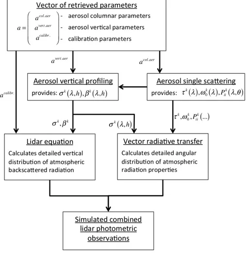
(10) Thèse de Valentyn Bovchaliuk, Lille 1, 2016. x 3.5.1 3.5.2 4. Methodologies to retrieve aerosol properties 4.1 Retrieval of optical properties . . . . . . . . . . . . . . . . . . . . . . . . . 4.1.1 Method which uses sun/sky-photometer primary measurements 4.1.2 Methods using LiDAR data . . . . . . . . . . . . . . . . . . . . . . a) Klett method . . . . . . . . . . . . . . . . . . . . . . . . . . . . . b) Raman method . . . . . . . . . . . . . . . . . . . . . . . . . . . . 4.1.3 Method combining sun-photometer and LiDAR measurements . 4.2 Retrieval of microphysical properties . . . . . . . . . . . . . . . . . . . . . 4.2.1 Inversion of sun/sky-photometer data . . . . . . . . . . . . . . . 4.2.2 Inversion of LiDAR data . . . . . . . . . . . . . . . . . . . . . . . . 4.2.3 Inversions based on synergy between sun/sky-photometer and LiDAR data . . . . . . . . . . . . . . . . . . . . . . . . . . . . . . . 4.3 GARRLiC algorithm . . . . . . . . . . . . . . . . . . . . . . . . . . . . . . 4.3.1 General description . . . . . . . . . . . . . . . . . . . . . . . . . . . Forward model . . . . . . . . . . . . . . . . . . . . . . . . . . . . . Numerical inversion . . . . . . . . . . . . . . . . . . . . . . . . . . 4.3.2 Enhancements implemented into the GARRLiC algorithm . . . . Molecular extinction and backscatter profiles . . . . . . . . . . . . New normalization procedure . . . . . . . . . . . . . . . . . . . . Conclusions and advantages . . . . . . . . . . . . . . . . . . . . .. 57 58 58 59 59 60 61 62 62 63 65 68 68 69 72 74 74 75 76. 5. Application of GARRLiC to data of SHADOW-2 (Phase 1) campaign 79 5.1 Comparison between Raman, LIRIC and Regularization retrievals . . . . 80 5.2 Conclusions . . . . . . . . . . . . . . . . . . . . . . . . . . . . . . . . . . . 96. 6. Water vapor mixing ratio profile. Calibration and application 6.1 Water vapor and Raman LiDAR measurements . . . . . . . . . . . . 6.2 LiDAR mixing ratio calibration . . . . . . . . . . . . . . . . . . . . . 6.2.1 Intercomparison with radiosonde measurements . . . . . . 6.2.2 Calibration by TWP using lunar-photometer measurements 6.2.3 Comparison of obtained calibration constants . . . . . . . . 6.3 Applications . . . . . . . . . . . . . . . . . . . . . . . . . . . . . . . . 6.3.1 Application to measurements over Lille site . . . . . . . . . 6.3.2 Application to measurements over Dakar site . . . . . . . . 6.4 Conclusions . . . . . . . . . . . . . . . . . . . . . . . . . . . . . . . .. 7. Conclusions and perspectives. Bibliography. © 2016 Tous droits réservés.. NMMB/BSC-Dust model . . . . . . . . . . . . . . . . . . . . . . . 54 HYSPLIT model . . . . . . . . . . . . . . . . . . . . . . . . . . . . . 54. . . . . . . . . .. . . . . . . . . .. . . . . . . . . .. 97 97 98 99 103 107 109 109 110 114 117 123. lilliad.univ-lille.fr.

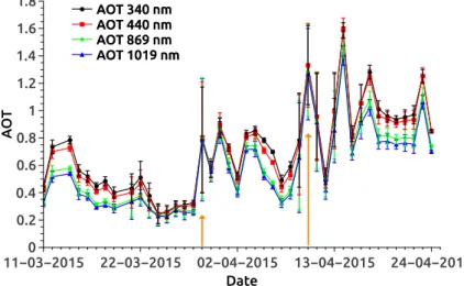
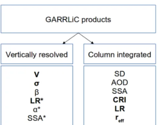
(11) Thèse de Valentyn Bovchaliuk, Lille 1, 2016. xi. List of Figures. © 2016 Tous droits réservés.. 1.1 1.2. Radiative forcing estimates by different constituents of the atmosphere . Aerosol influences on climate . . . . . . . . . . . . . . . . . . . . . . . . .. 2.1 2.2 2.3 2.4 2.5 2.6 2.7 2.8 2.9. Different aerosols collected at Lille and Dakar observational sites . . . Representation of differential solid angle . . . . . . . . . . . . . . . . . Spectral radiant flux . . . . . . . . . . . . . . . . . . . . . . . . . . . . . Solar spectrum on the top and bottom of the atmosphere . . . . . . . . Angular dependence of Rayleigh and Mie scattering . . . . . . . . . . . Schematic representation of light attenuation through the medium . . Representation of scattering phase function of the Rayleigh and Mie scattering . . . . . . . . . . . . . . . . . . . . . . . . . . . . . . . . . . . . Standard LiDAR setup . . . . . . . . . . . . . . . . . . . . . . . . . . . . Illustration of LiDAR geometry . . . . . . . . . . . . . . . . . . . . . . .. 3.1 3.2 3.3 3.4 3.5 3.6 3.7 3.8 3.9. LILAS photo at Lille site . . . . . . . . . . . . . . . . . . . . . . . . . . . . LILAS and CAML (CIMEL) beams at Dakar site during the observation LILAS optical scheme . . . . . . . . . . . . . . . . . . . . . . . . . . . . . . EARLINET check up: Rayleigh fit . . . . . . . . . . . . . . . . . . . . . . . EARLINET check up: telecover test . . . . . . . . . . . . . . . . . . . . . . Example of Volume Depolarization Ratio, quick look . . . . . . . . . . . Example of volume depolarization ratio, profile . . . . . . . . . . . . . . Example of LILAS data level 1.0 . . . . . . . . . . . . . . . . . . . . . . . . Example of LILAS data gluing . . . . . . . . . . . . . . . . . . . . . . . . .. 43 44 44 45 46 47 48 50 52. 4.1 4.2 4.3 4.4 4.5 4.6. Sun-photometer almucantar and principle plane geometries . . . . . . GARRLiC inversion structure . . . . . . . . . . . . . . . . . . . . . . . . GARRLiC products derived using single or two mode inversion . . . . Modeling of two aerosol components in GARRLiC algorithm . . . . . . GARRLiC general scheme . . . . . . . . . . . . . . . . . . . . . . . . . . GARRLiC assumption on aerosol volume concentration above and below trustworthy LiDAR altitude range . . . . . . . . . . . . . . . . . . .. 62 66 67 68 69. . . . . . .. 3 4 8 15 15 17 19 20. . 25 . 31 . 33. . . . . .. . 73. 5.1. AOD during SHADOW-2 Phase 1 . . . . . . . . . . . . . . . . . . . . . . . 80. 6.1 6.2 6.3 6.4 6.5 6.6. LILAS MR profile obtained using intercomparison calibration technique Calibration constants obtained using intercomparison technique . . . . . Calibration constants obtained using LP TPW calibration technique . . . LILAS MR profile obtained using LP TPW calibration technique . . . . . LILAS MR profiles obtained using both calibration techniques . . . . . . Height–temporal distribution of LILAS MR over Lille on 25 November 2014 . . . . . . . . . . . . . . . . . . . . . . . . . . . . . . . . . . . . . . . .. 101 102 106 106 108 109. lilliad.univ-lille.fr.

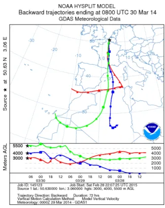
(12) Thèse de Valentyn Bovchaliuk, Lille 1, 2016. xii 6.7 6.8 6.9. Back trajectory for Lille site at 04:00 UTC, 25 November 2014 . . . . . . . 110 LILAS MR profile on 25 November 2014 . . . . . . . . . . . . . . . . . . . 110 Height–temporal distribution of AOT, mixing ratio, particle depolarization ratio, and LiDAR ratio over Dakar on 15–16 March 2015 . . . . . . . 112 6.11 Height–temporal distribution of LILAS MR over Dakar on 16 March 2015113 6.12 LILAS MR profile on 16 April 2015 . . . . . . . . . . . . . . . . . . . . . . 114. © 2016 Tous droits réservés.. lilliad.univ-lille.fr.

(13) Thèse de Valentyn Bovchaliuk, Lille 1, 2016. xiii. List of Tables. © 2016 Tous droits réservés.. 2.1. Typical properties for different wet and dry aerosol types . . . . . . . . . 12. 4.1. Typical Raman LR at 532 nm for different aerosol types . . . . . . . . . . 61. 6.1. Calibration constants and TPW obtained using intercomparison and LP TWP calibration techniques . . . . . . . . . . . . . . . . . . . . . . . . . . 107. lilliad.univ-lille.fr.


(15) Thèse de Valentyn Bovchaliuk, Lille 1, 2016. xv. List of Abbreviations LOA CaPPA SHADOW-2 LILAS LIRIC GARRLiC AERONET EARLINET MPLINET LALINET ADNET GAW GALION NDACC RF POM VOC OC BC CCN TOA MODIS PLASMA NMMB/BSC-Dust HYSPLIT GDAS NOAA LR LS AE SD CRI AOD SSA TWP WV RCS LSM. © 2016 Tous droits réservés.. Laboratoire d’Optique Atmosphérique Chemical and Physical Properties of the Atmosphere Study Saharan dust over the West Africa second campaign Lille LIDAR AtmosphereS LIDAR-Radiometer Inversion Code Generalized Aerosol Retrieval from Radiometer and LIDAR Combined data Aerosol Robotic Network European Aerosol Research LIDAR Network Micro-Pulse LIDAR Network Latin American LIDAR Network Asian Dust Network Global Atmosphere Watch Global Aerosol LIDAR Observation Network Network for the Detection of Atmospheric Composition Change Radiative Forcing Particles of organic matters Volatile organic compounds Organic carbon Black carbon Cloud condensation nuclei Top of Atmosphere Moderate Resolution Imaging Spectroradiometer Photométre Léger Aéroporté pour la Surveillance des Masses d’Air Non-hydrostatic Multiscale Model, Barcelona Supercomputing Center Hybrid Single-Particle Lagrangian Integrated Trajectory Global Data Assimilation System National Oceanic and Atmospheric Administration LIDAR ratio LIDAR signal Angström exponent Size distribution Complex refractive idex Aerosol optical depth Single scattering albedo Total precipitable water Water vapor Range corrected signal Least square method. lilliad.univ-lille.fr.

(16) Thèse de Valentyn Bovchaliuk, Lille 1, 2016. xvi. © 2016 Tous droits réservés.. lilliad.univ-lille.fr.

(17) Thèse de Valentyn Bovchaliuk, Lille 1, 2016. xvii. List of Symbols. © 2016 Tous droits réservés.. λ. wavelength. nm. σ ext. extinction coefficient. m−1. σ sca. scattering coefficient. m−1. σ sca,cs. scattering cross section coefficient. m2 sr−1. σ abs. absorption coefficient. m−1. Qabs. absorption efficiency factor. Qsca. scattering efficiency factor. β. backscatter coefficient. ω0. single scattering albedo. θ0. zenith angle. o , deg. θ. scattering angle. o , deg. P (θ). phase matrix. P11 (θ). scattering phase function. δ. depolarization ratio. α. Angström exponent. αext. extinction Angström exponent. τ. optical thickness. m0. relative air mass. ref f. effective radius. µm. Ω. solid angle. sr. Φe. radiant flux. W or J/s. Φλ. spectral flux. W/nm−1. Iλ. spectral intensity. W sr−1 nm−1. Lλ. spectral radiance. W/(m2 sr nm). x. size parameter. m. complex refractive index. n. real part of complex refractive index (RRI). k. imaginary part of complex refractive index (IRI). N (r). number particle size distribution. µm−2. S(r). surface particle size distribution. m2 µm−2. m−1 sr−1. lilliad.univ-lille.fr.

(18) Thèse de Valentyn Bovchaliuk, Lille 1, 2016. xviii volume particle size distribution. µm3 µm−2. V. volume of particles. µm3 µm−3. N. number concentration. m−3. TPW. total precipitable water content. cm, g cm−1. wnc (z). not calibrated mixing ratio profile. w(z). water vapor mixing ratio. g kg −1. e(z). profile of water vapor pressure. Pa. ew (z). profile of saturation water pressure. Pa. ρH2 O,air (z). water vapor and air densities. g m−3. C1. MR calibration constant using intercomparison technique. C2. MR calibration constant using LP TWP technique. P (R). power of backscattered radiation from distance R. K. factor of LiDAR performance. G(R). factor of range dependent geometry. T (R). atmosphere transmittance. Pbg. power of background noise. V dp. calibration constant of depolarization coefficient. V (r) =. dV d ln(r). mV. coefficients of beam-splitter cube:. © 2016 Tous droits réservés.. Tp. for parallel light transmittance. Ts. for perpendicular light transmittance. Rp. for parallel light reflectance. Rs. for perpendicular light reflectance. lilliad.univ-lille.fr.

(19) Thèse de Valentyn Bovchaliuk, Lille 1, 2016. 1. Chapter 1. Introduction 1.1. Introduction. The globally averaged surface temperature of the Earth calculated by the linear trend shows a warming of 0.85 o C over the period from 1880 to 2012, and global surface temperature change for the end of the 21st century is likely to exceed 1.5 o C (Stocker et al., 2013). Temperature can be critical as it influences our world, where everyhting is interconnected. The temperature increase has been attributed to changes in the concentrations of greenhouse gases (Stocker et al., 2013). These atmospheric constituencies are attributed to human activities; therefore it is possible to influence on their concentrations and globally "control" Earth’s atmosphere system. The Earth’s atmosphere consists of gases and particles. There are two groups of gases, with nearly steady and with variable concentrations. Gases with residence times greater than about a decade are considered to be long-lived. Through the mixing and circulation of the atmosphere, these gases have concentrations that are to some extent uniform. Gases with short residence times, such as water vapor and ozone, are considered to be short-lived. They have high concentrations near their sources and low ones near their sinks (Coakley Jr. and Yang, 2014). There is very high confidence that well mixed greenhouse gases positively contribute to radiative forcing estimates (Fig. 1.1), which is defined as a net change of incoming and outgoing energy in the Earth’s atmosphere system. Human activities are the main source of the additional greenhouse gases in the atmosphere, thus, by controlling emission of greenhouse gases we could warm up or cool down the atmosphere (Coakley Jr. and Yang, 2014).. © 2016 Tous droits réservés.. lilliad.univ-lille.fr.

(20) Thèse de Valentyn Bovchaliuk, Lille 1, 2016. 2. Chapter 1. Introduction. Atmospheric components such as clouds and aerosol particles are highly variable in space and time. Aerosols are solid/liquid particles suspended in the atmosphere. Because of a wide variety of aerosols, it differently interacts with radiation. That is the main reason why during last decade significance of aerosol studies stays very vital. Aerosol analysis is complex and requires a lot of resources due to a wide variety of particle types and theirs mixtures. That is why, according to Stocker et al., 2013 aerosol still contribute the largest uncertainties in total radiative forcing estimates. Many efforts have been devoted to aerosol studies for better understanding their impacts on a climate. According to Stocker et al., 2013, the radiative forcing of the total aerosol effect in the atmosphere, which includes cloud adjustments due to aerosols, is -0.9 [-1.9 to -0.1] W m−2 (medium confidence). As it is seen from Fig. 1.1, most of the aerosols have negative forcing, and only positive contribution comes from black carbon, which absorbs solar radiation. There is high confidence that aerosols and their interactions with clouds have offset a substantial portion of global mean forcing from well-mixed greenhouse gases. Radiative forcing due to anthropogenic activities estimates in 2011 relative to 1750 is 2.29 [1.13 to 3.33] W m−2 (Fig. 1.1). It has increased more rapidly since 1970, relative anthropogenic RF in 1970 to 1750 is 0.57 [0.29 to 0.85] W m−2 . RF estimates in 2011 is 43% higher than reported in 2007 (IPCC, 2007), it was reported 1.6 [0.6 to 2.4] W m−2 . It is explained by continuing growth of greenhouse gas concentration and due to improved RF estimate. Generally, it brings warming of the atmosphere and the ocean, in changes in the global water cycle, in reductions in snow and ice, etc. Aerosols influence on climate can be divided into direct, indirect, and semi-direct effects (Fig. 1.2). Aerosols directly interact with radiation by scattering and absorbing mechanisms, and therefore, may result in warming or cooling of the atmosphere. If the total RF is positive in the atmosphere column it warms up the atmosphere, and if the total radiative forcing is negative it cools off the atmosphere. Warming and cooling processes depend on aerosols single scattering albedo and on the albedo of underlying surface (Haywood and Boucher, 2000). Indirect effect consists in aerosols influence on cloud lifetime, height, albedo, and other cloud properties. The indirect influence can be divided into Twomey (Twomey,. © 2016 Tous droits réservés.. lilliad.univ-lille.fr.

(21) Thèse de Valentyn Bovchaliuk, Lille 1, 2016. 1.1. Introduction. 3. F IGURE 1.1: Radiative forcing estimates in 2011 relative to 1750 and aggregated uncertainties for the primary drivers of climate change. Values are global average radiative forcing, partitioned according to the emitted compounds or processes that result in a combination of drivers. The best estimates of the net radiative forcing are shown as black diamonds with corresponding uncertainty intervals. The numerical values are provided on the right of the figure, together with the confidence level in the net forcing (VH - very high, H - high, M - medium, L - low, VL - very low). Albedo forcing due to black carbon on snow and ice is included in the black carbon aerosol bar. Small forcings due to contrails (0.05 W m−2 , including contrail induced cirrus), and HFCs, PFCs and SF 6 (total 0.03 W m−2 ) are not shown. Concentration-based RFs for gases can be obtained by summing the like-colored bars. Volcanic forcing is not included as its episodic nature makes it difficult to compare to other forcing mechanisms. Total anthropogenic radiative forcing is provided for three different years relative to 1750. Figure is taken from the summary for policymakers (Stocker et al., 2013).. 1974; Twomey, 1977) and Albrecht (Albrecht, 1989) effects. In Twomey effect, the aerosols provide an additional nuclei for droplet or ice crystal growth (Twomey, 1974; Boucher, 1999; Lohmann, Kärcher, and Timmreck, 2003) and change the cloud albedo. In Albrecht effect, aerosols can change lifetime of clouds, liquid water content and top height of clouds (Albrecht, 1989; Pincus and Baker, 1994). Indirect effects depend on concentration and type of aerosols and clouds (Kaufman, Tanré, and Boucher, 2002;. © 2016 Tous droits réservés.. lilliad.univ-lille.fr.

(22) Thèse de Valentyn Bovchaliuk, Lille 1, 2016. 4. Chapter 1. Introduction. Lohmann and Feichter, 2005). Semi-direct effect consists in temperature profile modification by absorbing aerosols (Johnson, Shine, and Forster, 2004; Koch and Del Genio, 2010). Some tropospheric aerosols can absorb shortwave radiation and heat the atmosphere, it affects the relative humidity and stability of troposphere, and, thereby, influences on cloud formation and lifetime.. F IGURE 1.2: Schematic diagram showing the various radiative mechanisms associated with cloud effects that have been identified as significant in relation to aerosol (modified from Haywood and Boucher, 2000).. The uncertainties in estimation of the aerosols effects on RF are still high (Fig. 1.1) according to IPCC, 2007; IPCC, 2013. Improvements of observations, development of instrumentation and modeling are the main sources of enhancements in aerosol forcing estimations. Under conditions of high relative humidity, an aerosol particle may growth due to the water uptake (hygroscopic growth) modifying aerosols size distribution. Water vapor (WV) affects the direct scattering of radiation (Hänel, 1976) and especially the indirect effects, the aerosol water uptake is highly related to their ability to act as cloud condensation nuclei (CCN) (Charlson et al., 1992). Thus, a better knowledge of WV content and relative humidity are in high importance of aerosol studies, in particular, their vertical distribution.. © 2016 Tous droits réservés.. lilliad.univ-lille.fr.

(23) Thèse de Valentyn Bovchaliuk, Lille 1, 2016. 1.2. Objectives and outline of the thesis. 1.2. 5. Objectives and outline of the thesis. Hence, during the thesis newly developed multi-wavelength Raman-polarization LiDAR called LILAS (LIlle LiDAR AtmosphereS) was built, set up and used for measurements. Observations were carried out in West Africa and the adjacent oceanic region (SHADOW-2 campaign - a study of SaHAran Dust Over West Africa) which is very consequential location for studying dust properties. Some improvements have been implemented into the GARRLiC algorithm (Generalized Aerosol Retrieval from Radiometer and LiDAR Combined data) which were used for data analyses. Therefore, the first objective of the thesis was to build, set up and characterize a new multiwavelength Raman-polarization LiDAR system. The second objective of the thesis consisted in an implementation of several improvements into the GARRLiC algorithm and in analyses of aerosol retrievals in terms of aerosol optical and microphysical properties. LILAS direct measurements provide water vapor mixing ratio profile, which is a suitable tracer that indicates the boundary between dry air masses transported over the continent and moist air masses coming from the ocean. As we already mentionned it, WV vertical distribution is of high importance for aerosol studies. Therefore, last part of the thesis concerns the developed LILAS calibration techniques for water vapor mixing ratio measurements. The thesis report is organized as followed: • Chapter 2 is devoted to the description of basic concepts of aerosols, light scattering theory and fundamentals of lidar technique. • Chapter 3 describes instruments which were used for the thesis and the observational sites in which measurements were carried out. Particular emphasis is made on LILAS LiDAR, its general description, its quality assurance procedures, its operation, and measurements. The procedure for processing the level 1.0 data from the raw data developed during the thesis, is described.. © 2016 Tous droits réservés.. lilliad.univ-lille.fr.

(24) Thèse de Valentyn Bovchaliuk, Lille 1, 2016. 6. Chapter 1. Introduction • Chapter 4 describes the methodologies which were used to obtain aerosol properties. Special emphasis is made on GARRLiC algorithm and on its enhancements implemented during the thesis. • Chapter 5 presents the results of an application of the various methods described in Chapter 4. Results of GARRLiC application on LiDAR data which were carried out during SHADOW 2 campaign are presented and included as a paper (Bovchaliuk et al., 2016) published in Atmospheric Measurements Technique journal. • Chapter 6 presents and discusses calibration techniques for LILAS measurements of water vapor mixing ratio. These calibration techniques were developed considering observational sites specification (distance between LiDAR and radiosonde measurements and lunar-photometer observation). The derived calibration constants were used in the application on LILAS measurements and are presented in the end of the chapter. • The manuscript ends with conclusions and perspectives.. © 2016 Tous droits réservés.. lilliad.univ-lille.fr.

(25) Thèse de Valentyn Bovchaliuk, Lille 1, 2016. 7. Chapter 2. Fundamentals 2.1. Aerosols and climate. Science and society are interested in aerosols for many reasons. High aerosol concentration can cause serious health hazard and have been linked to increasing in morbidity and mortality rates, and degradation of environmental quality concerning of air quality (Amiridis et al., 2012), acid rain and reduction of visibility (Lenoble, Remer, and Tanré, 2013). The decrease of visibility due to high attenuation by the aerosols is a grave concern for some military or civil sighting. Volcanic ash emissions can cause breakage of jet engines and disruption of air traffic (Kienle et al., 1990). In the polar regions aerosols play a major role in the heterogeneous atmospheric chemistry, in stratospheric clouds, they can depress ozone concentration (Andreae and Crutzen, 1997). However, one of the main reason of interest is aerosols influence on Earth’s climate. They influence the energy budget and cause climate changes on the regional and global scales (Lenoble, Remer, and Tanré, 2013; IPCC, 2007; IPCC, 2013). As was mentioned above, their impacts can be divided in direct, indirect and semi-direct effects. By these effects aerosols increase/decrease energy budget and cause the Earth’s atmosphere warming/cooling. Huge efforts are being performed to study aerosol effects on Earth’s climate. The total aerosol effect in the atmosphere is -0.9 [-1.9 to -0.1] W m−2 (IPCC, 2013), the uncertainties in the aerosol radiative forcing have been reduced with respect to IPCC, 2007. However, aerosol forcing continues contribute the largest uncertainties to the total radiative forcing estimate.. © 2016 Tous droits réservés.. lilliad.univ-lille.fr.

(26) Thèse de Valentyn Bovchaliuk, Lille 1, 2016. 8. Chapter 2. Fundamentals. Aerosols are solid and/or liquid particles suspended in the atmosphere with the exception of clouds. We notice their presence because they scatter and absorb the sunlight. In case of high concentration, they can be seen as haze, smoke from fires, dust storm, etc. Most aerosols are concentrated in boundary layer near production sources. However, they can be lifted by air-masses up to 4-6 km in altitude and transported over long distances. In case of volcanic eruption or huge forest fires they can reach 10-12 km, and even higher altitudes in the stratosphere. Aerosol particles can be divided into two categories: (i) natural, formed by wind, erosion, volcanic eruptions and other natural processes; and (ii) anthropogenic, caused by human activities (Lenoble, Remer, and Tanré, 2013). Particles are removed from the atmosphere by dry deposition, evaporation, and settling with precipitation. Those, which have been emitted directly into atmosphere are called primary aerosol, and the ones formed by gas to particle conversion processes are called secondary aerosols. The size range of aerosol particles varies from few nanometers to tens of micrometers in diameter (Seinfeld and Pandis, 2006). Liquid particles are approximately spherical, whereas solid aerosols have different shapes (see Fig. 2.1). The time of the aerosol residence in the atmosphere varies from minutes for smallest particles that are coagulating rapidly to years for stratospheric particles.. F IGURE 2.1: Wide variety of aerosol and their shapes, from left to right: soot collected at Lille, 29 March 2014; metallic (Iron) surrounded by a shell gathered at Lille, 13 March 2014; dust (Aluminum silicate) received at M’Bour at 2 km altitude during the flight, 10 April 2015; fresh sea salt (NaCl) collected at M’Bour during SHADOW-2 campaign at 3 km altitude during the flight, 10 April 2015 (Pictures from Choël Marie and Florin Unga, LASIR/LOA, 2015).. © 2016 Tous droits réservés.. lilliad.univ-lille.fr.

(27) Thèse de Valentyn Bovchaliuk, Lille 1, 2016. 2.1. Aerosols and climate. 2.1.1. 9. How to observe aerosols?. In situ and remote sensing measurements are two ways to observe the aerosols. The former is by means through direct interaction with particles at the point of observation. The latter allows measure aerosol properties from a distant point without direct interaction. Remote sensing can be categorized into "active" and "passive" techniques depending on instrumental design. Instruments used for passive remote sensing measures the properties of radiation scattered by particles and molecules whereas active instruments measure the scattered radiation emitted by themselves (the radiation source is a part of the system). Ground based remote sensing techniques provide accurate results for aerosol characterization (Dubovik and King, 2000; Dubovik et al., 2011; Olmo et al., 2006; Klett, 1981; Ansmann, Riebesell, and Weitkamp, 1990). They provide aerosol properties at local scale. Observing networks have been established using systems with the same or similar measurement techniques to be more efficient and aiming to provide global coverage. Among such networks are EARLINET (European Aerosol Research Lidar Network, www.earlinet.org) (Pappalardo et al., 2014), MPLINET (MicroPulse Lidar Network) (Welton et al., 2001; Welton et al., 2005), LALINET (Latin American Lidar Network, www.lalinet.org) (Guerrero-Rascado et al., 2014), ADNET (Asian Dust Network) (Murayama et al., 2001), SKYNET (Takamura, Nakajima, et al., 2004) and AERONET (Aerosol Robotic Network, http://aeronet.gsfc.nasa. gov/) (Holben et al., 1998). Also, there is one global aerosol LiDAR network of networks, the GAW (Global Atmosphere Watch) Aerosol Lidar Observation Network (GALION). GALION does not consist of a uniform set of LiDAR systems which are sparsed through the Earth at different stations, but makes use of existing systems in already established stations, of the experienced operators of these systems, and of existing network structures. GALION includes EARLINET, NDACC (Network for the Detection of Atmospheric Composition Change), ADNET and MPLNET (Bösenberg et al., 2007). Aerosol vertical distribution is important for radiative forcing estimation, especially for accounting indirect and semi-direct aerosol effects (Claquin et al., 1998; Meloni et. © 2016 Tous droits réservés.. lilliad.univ-lille.fr.

(28) Thèse de Valentyn Bovchaliuk, Lille 1, 2016. 10. Chapter 2. Fundamentals. al., 2005; Samset et al., 2013). LiDAR instruments are very useful tool for the determination of the aerosol vertical distribution. Such systems are widely used, and variety of LiDAR techniques have been developed for aerosol studies (Klett, 1981; Ansmann, Riebesell, and Weitkamp, 1990; Shipley et al., 1983; Weitkamp, 2005). Depending on LiDAR capabilities, optical and/or microphysical aerosol properties can be derived. Extinction (σ), backscatter (β) and extinction to backscatter ratio (σ/β), so called LiDAR ratio (LR), coefficients refer to optical aerosol properties, whereas aerosol effective radius (ref f ), size distribution (SD), volume (V), mass, surface-area (S), number (N) concentrations and complex refractive index (CRI) are belonging to microphysical properties. There are several methods used to retrieve aerosol properties from LiDAR measurements. However, in general, they can be divided into three main groups (Weitkamp, 2005). The methods from the first group are combining measurements from several different instruments. A preferred approach is to combine lidar and sun-photometer observations. In this case, the treatment of the data is more straightforward, the latter delivers integrated optical depths of the atmospheric column at multiple wavelengths. In the second group, the optical properties like σ and β are calculated by Mie-theory and then are compared with the corresponding properties obtained from Raman LiDAR technique (Wandinger et al., 1995; Barnaba and Gobbi, 2001). Optical properties are calculated using a priori assumptions. The application of these methods has been restricted to special cases (polar stratospheric clouds, ejecta from volcanic eruptions and other atmospheric processes with well-known type of particles) because of the uncertainties associated with such a priori assumptions. The third group, derived from the second one, aims at (i) reducing number of a priori constraints, and (ii) improving the ability to retrieve aerosol properties in the highly variable tropospheric conditions. These retrieval approaches consist of mathematical methods that use spectral LiDAR information (Uthe, 1982; Müller, Wandinger, and Ansmann, 1999; Veselovskii et al., 2002; Veselovskii et al., 2012; Shcherbakov, 2007). More detailed descriptions will be presented in Chapter 4.. © 2016 Tous droits réservés.. lilliad.univ-lille.fr.

(29) Thèse de Valentyn Bovchaliuk, Lille 1, 2016. 2.1. Aerosols and climate. 2.1.2. 11. Aerosol types. The term "aerosols" by itself is not well defined because of a wide variety of substances by which aerosols are presented. Even sub-classifications of aerosols such as dust or smoke are themselves generic terms because of many combinations of minerals or organics respectively (Lenoble, Remer, and Tanré, 2013). That is why, aerosols can be classified in many terms, according to their chemical composition, mechanism of formation, origin or size of particles. According to aerosols origin, they can be devided into natural and anthropogenic. Natural aerosols includes sea salt, desert dust, volcanic and biogenic emissions, a smoke of wildfires, and biomass burning. Anthropogenic aerosols caused by a human activity, which includes industrial emission, biomass burning for agriculture, land erosion and evaporation of lakes caused by human. According to formation mechanisms, particles which have been emitted directly into atmosphere are called primary aerosols, and the ones formed by a gas to particle conversion processes are called secondary aerosols. Regarding particle size, they can be divided in fine and coarse mode particles. Fine mode particles have diameter <1 µm, and consist of nucleation or Aitken mode, formed with particles in diameter range from 0.001 to 0.1 µm, and accumulation mode with diameters between 0.1 and 1 µm (Eck et al., 2010). Coarse mode particles have diameter in range from 1 to 100 µm, but most of coarse aerosol mass contained in range from 1 to 10 µm (Lenoble, Remer, and Tanré, 2013). Aerosol optical properties, which are radiative characteristics, depend on the chemical composition of particles, their sizes and shapes. The composition is represented by the complex refractive indices (CRI), with the real (RRI) and imaginary (IRI) parts contributing to the determination their scattering and absorption properties. These properties can be measured in the laboratory or by in situ instrumentation during a campaign or at observational sites. In this case, such measurements will represent dry aerosol properties and not necessarily the ambient properties of aerosol layer, since several substances are hygroscopic. Some types of aerosols are easily combined with water vapor forming liquid particles with new optical and microphysical properties. At best, aerosol can be divided into such types: (i) Sulfates; (ii) Black Carbon (BC); (iii). © 2016 Tous droits réservés.. lilliad.univ-lille.fr.

(30) Thèse de Valentyn Bovchaliuk, Lille 1, 2016. 12. Chapter 2. Fundamentals. Particles of Organic Matters (POM); (iv) Dust; and (v) Sea Salt. These aerosol types are also used in climatological models, which form aerosol from estimates of source emissions, then allow the particles to be transported by modeled meteorology, transformed from modeled chemical processes and removed from the atmosphere by modeled wet and dry deposition. In Table 2.1 presented physical properties of dry and wet particles (Lenoble, Remer, and Tanré, 2013). In the following subsection anthropogenic pollution, biomass burning and mineral dust are described with more details. Physical property. Sulfate. BC. POM. Dust. Sea salt. Real part of refractive index (dry) Imaginary part of refractive index (dry). ∼1.53. ∼1.75. ∼1.53. ∼1.53. ∼1.50. ∼0.005. ∼0.440. ∼0.006. ∼0.008. ∼0.000. Real part of refractive index (wet) Imaginary part of refractive index (wet). 1.35–1.45. 1.35–1.45. 1.48. 1.35-1.45. ∼0.002. ∼0.003. ∼0.005. ∼0.000. Effective radius in µm Shape. 0.1–0.2 sphere. 0.1–0.2 sphere. 1.5–3.0 not sphere. ∼1 sphere. *not sphere. TABLE 2.1: Approximate typical physical properties for different aerosol types. Refractive index presented to 550nm, table taken from (Lenoble, Remer, and Tanré, 2013). *Black carbon (BC) originated as long non-spherical chains, but those chains collapse and are often incorporated in other organic matters (POM) that adds coating over the collapsed BC chains. Rarely BC is seen in its pure state in the real atmosphere.. Anthropogenic pollutions Traffic and industrial emissions are the greatest sources of anthropogenic pollution, as well as particles originated from precursor gases (SO2 , N O, N H4 and volatile organic compounds or VOC). According to the size, they belong to fine mode particles and present spherical shape. These particles are small and that is why they can be transported far from their sources. Particles lifetime, in the atmosphere, varies from several to 15 days.. © 2016 Tous droits réservés.. lilliad.univ-lille.fr.

(31) Thèse de Valentyn Bovchaliuk, Lille 1, 2016. 2.1. Aerosols and climate. 13. Primary anthropogenic aerosols compound from Organic Carbon (OC, generates during decaying vegetation, bacterial growth, and other natural processes) and Black Carbon (BC, forms by fossil flues, biomass burning, mainly from anthropogenic origin) (Bond et al., 2007). Secondary aerosol particles, which are originated from precursor gases, mainly compounds from sulfates and nitrates. Sulfates are generated from the oxidation of SO2 (thermal power plants and industrial activities are emitting sulfates), and nitrates are formed from oxidation of N Ox (traffic and industrial activities are emitting nitrates).. Biomass Burning aerosols Biomass burning describes the burning of living and dead vegetation. Burning can be caused by anthropogenic (land clearing for further use) and natural (wildfires are also frequent) reasons. Biomass burning aerosols consist of two major chemical components: BC which primarily absorbs solar radiation and OC which primarily scatters solar radiation. Both usually have a high fine mode contribution. Black carbon originated as long nonspherical chains, but those chains collapse and are often incorporated in other organic matters that adds coating over the collapsed BC chains. Hence, particle properties of both OC and BC are strongly varied depending on the burning process or the processes during the transport (hygroscopic growth, coagulation or photochemical mechanisms, etc.) (Amiridis et al., 2009a; Ancellet et al., 2016; Müller et al., 2007).. Mineral Dust Mineral dust particles are non-spherical with highly irregular shapes (Fig. 2.1). The size of particles can vary from 0.4 µm to tens of micrometers. Dust particles are picked up by wind erosion and can be transported at huge distances. For instance, the Saharan dust has formed the coast of Florida (Prospero, 1996; Joseph, 1999; Muhs et al., 2007). But in the same time, because of high weight, the lifetime of the dust aerosols is small, and most of the particles are settling down in few days (up to 7) (Lenoble, Remer, and Tanré, 2013; Freudenthaler et al., 2009). Besides the natural sources, dust. © 2016 Tous droits réservés.. lilliad.univ-lille.fr.

(32) Thèse de Valentyn Bovchaliuk, Lille 1, 2016. 14. Chapter 2. Fundamentals. emission is assumed to have a significant anthropogenic component mainly originating from agricultural and industrial practices. Some authors estimate the contribution of anthropogenic dust into annual dust emission about 50-70% (Washington et al., 2003), the annual emission is about 1600 [700-4000] Tg/year. There are a lot of mineral dust sources around the word, among them are Sahara desert in Northern Africa, Wahiba Sands in the Middle East, Makran coastal zone and a broad area of central Pakistan in Southwest Asia, Tarim Basin, Gobi and Mongolia region in China, Mojave and Colorado deserts in North America, etc. In view of the fact that mineral dust has high annual emission and global coverage, it has global climate effect. This effect is complex, because of wide variety of particle sizes and theirs chemical composition (Al, Si, Fe, Ti, non-sea-salt (nss) Ca, nssNa, and nssK) which scatter and absorb long-wave terrestrial radiation (Marconi et al., 2014; Tanré et al., 2003). The magnitude and the sign of dust RF strongly depend on a composition of particle mixture, but, generally, the mineral dust has a cooling effect. Depending on the season, dust may be mixed with biomass burning aerosols; it results in single scattering albedo that states the sign of the direct RF effect. An important role on dust radiative estimates also plays vertical distribution of particles (Sokolik et al., 2001). Because of their irregular shapes, the application of randomly oriented spheroids is usually used to describe dust particles (Mishchenko et al., 1997; Mishchenko, 2014; Veselovskii et al., 2010).. 2.2. Basic radiometric quantities. Radiative energy transfer is the physical phenomenon of energy transfer in the form of electromagnetic radiation. This phenomenon is responsible for radiative transfer in the atmosphere. The analysis of a radiation field often requires the consideration of radiant energy within one elementary solid angle dΩ. A differential solid angle is defined as a ratio of the differential area dS of a spherical surface intercepted to the square of the radius r: dΩ = dS/r2 = sinθ0 dθ0 dϕ, θ0 and ϕ denote to zenith and azimuthal angles (see Fig. 2.2).. © 2016 Tous droits réservés.. lilliad.univ-lille.fr.

(33) Thèse de Valentyn Bovchaliuk, Lille 1, 2016. 2.2. Basic radiometric quantities. 15. F IGURE 2.2: Illustration of a differential solid angle dΩ. Also shown for demonstrative purpose an element of area dA in directions confined to an element of solid angle dΩ.. Radiant flux (Φe ) is defined by total radiant energy per unit time. It does not contain any information on spectral or directional distribution of radiation. Radiant flux is measured in the watts (W ). Spectral flux (Φλ ) is radiant flux (Φe ) per unit of wavelength (Fig. 2.3). Spectral flux is defined by the radiant energy within wavelength interval (λ, λ + dλ) and the unit is W nm−1 . Radiant flux can be obtained through integration of spectral flux within all wavelengths:. Z Φe =. Φλ (λ)dλ. (2.1). F IGURE 2.3: Relation between spectral radiant flux Φλ and radiant flux Φe , visualized at a hypothetical example. Radiant flux emitted in the wavelength interval (λ, λ + dλ) is given by the area of the rectangle, which amounts to Φλ (λ)dλ. The total amount of radiant flux Φe emitted over the whole spectrum is given by the area under the curve. Figure taken from http://light-measurement.com/ basic-radiometric-quantities/.. © 2016 Tous droits réservés.. lilliad.univ-lille.fr.

(34) Thèse de Valentyn Bovchaliuk, Lille 1, 2016. 16. Chapter 2. Fundamentals. Spectral intensity (Iλ ) is spectral flux per unit solid angle (dΩ), the unit of spectral intensity is W sr−1 nm−1 :. dΦλ dΩ. Iλ =. (2.2). Hence, spectral flux can be defined regarding spectral intensity:. Z Iλ dΩ. Φλ =. (2.3). Ω. Spectral radiance (Lλ ) is spectral intensity which is passing through unit surface dA in direction confident to solid angle dΩ which is oriented to the normal of dA in an angle θ0 (Fig. 2.2):. Lλ =. dIλ cos(θ0 ) dA. (2.4). In terms of spectral flux, spectral radiance can be written as:. Lλ =. dΦλ cos(θ0 ) dA dΩ. (2.5). The unit of spectral radiance is W m−2 sr−1 nm−1 .. 2.3. Light scattering and absorption by atmospheric molecules and aerosols. There are two processes (scattering and absorption) by which electromagnetic radiation interacts with atmospheric aerosol particles and molecules. As it was mentioned above, these two processes form direct aerosol effect on RF estimate in the Earth’s atmosphere, and the net aerosol effect indicate negative influence. As a result of absorption, the energy of incident light becomes part of the internal energy of particle/molecule. In case of molecules, absorption process is quantized. © 2016 Tous droits réservés.. lilliad.univ-lille.fr.

(35) Thèse de Valentyn Bovchaliuk, Lille 1, 2016. 2.3. Light scattering and absorption by atmospheric molecules and aerosols. 17. because it depends on rotational, vibrational of electronic energies of the molecule. Hence, we should have discrete absorption lines of atmosphere molecules, but there are number of effects which are shifting or broadening the line, such as thermal Doppler effect, pressure broadening effect and others. There are a variety of gases in Earth’s atmosphere and, therefore, not all solar energy reach the Earth’s surface. Solar spectrum on the top of the atmosphere and at sea level are presented in Fig. 2.4. The main molecular absorber are H2 O (water vapor), CO2 , O3 , N2 O, CO, O2 , CH4 , N2 . Most of them absorb solar energy in near- and far-infrared wavelength regions as it shown in Fig. 2.4, except ozone which absorbs mainly in near-ultraviolet wavelengths.. F IGURE 2.4: Solar spectrum on the top of atmosphere (1) and at the sea level (2). Absorption bands of various of gases are presented with identification of molecule; the shaded area correspond to the energy absorbed by various gases in a clear atmosphere. Figure is taken from Chapter 15 (Brasseur, Orlando, Tyndall, et al., 1999).. As a result of scattering, the incident light elastically or inelastically interacts with a particle/molecule. During this interaction, an energy of incident light is redistributed by scattering process. The term elastic scattering means that there is no difference between the wavelengths of the incident and scattered light. During the inelastic scattering some of the particle energy is lost or gained. It is, for example, the so called Raman scattering, by which rotational, vibrational and/or rotational-vibrational energy level of particle changes. For the Stokes Raman scattering, particle gains the energy. © 2016 Tous droits réservés.. lilliad.univ-lille.fr.

(36) Thèse de Valentyn Bovchaliuk, Lille 1, 2016. 18. Chapter 2. Fundamentals. (absorbed energy is higher than emitted one), and for anti-Stokes Raman scattering, particle loses the energy (absorbed energy is lower than emitted one). Consequently, for Stokes and anti-Stokes Raman scattering incident photon loses and gains the energy respectively. Wave-number shift caused by inelastic scattering can be calculated as (Weitkamp, 2005).. ∆ν =. ∆E hc0. (2.6). where ∆E is the difference between energy levels of the scattering molecule before and after the scattering, ∆ν = 1/λ = ν/c0 - wave-number of the scattered radiation, h and c0 - Planck constant and speed of light, respectively. For LiDAR observations, Raman effect is widely used to obtain concentration profiles of specific molecules. The process of scattering is highly depends on refractive index (m = n + ik) and size parameter (x), which characterized by the ratio of particle radius (r, particle length) and wavelength of incident light (λ), if particles are spherical:. x = 2πr/λ. (2.7). Rayleigh theory is used if size parameter and real part of refractive index (n) meets the requirement x < 0.6/n. This theory is used to describe molecular scattering. Rayleigh theory is based on the assumption that all particles are spherical and their radii are much smaller than the wavelength of incident light. Rayleigh scattering coefficient depends on wavelength, and in general form like ∼ λ−4 . Mie theory is used when the size parameter and real part of the refractive index (n) satisfy the requirement 0.6/n < x < 5. This theory is used when radii of particles are comparable with the wavelength of incident light. Scattered light has strong angular dependency, which is prominent in forward direction. Mie scattering is a more general theory and it is converges into Rayleigh theory with size parameter decreasing. Rayleigh theory is much simpler in computational implementation. It should be noted, Mie theory is applied only to spherical particles.. © 2016 Tous droits réservés.. lilliad.univ-lille.fr.

(37) Thèse de Valentyn Bovchaliuk, Lille 1, 2016. 2.3. Light scattering and absorption by atmospheric molecules and aerosols. 19. Geometric optics approximation is used if size parameter is larger than 5 (x > 5). Such type of scattering is mainly a process of reflection and refraction. Geometrical optics is associated with "real" rays, but their analytic continuation to complex values of some associated parameters enables the concept of "complex rays" to be used, often in connection with surface or "evanescent" rays traveling along a boundary while penetrating the less dense medium in an exponentially damped manner (Adam, 2015). Light scattering strongly depends on scattering angle θ. It is the angle between incident and scattered direction. In case of θ = 0o , scattered light propagates in the same direction as incident light (forward direction). In the event of θ = 180o , scattered light propagates in a backward direction. LiDARs measure the light which is backward scattered. Figure 2.5 shows differences between Rayleigh and Mie scattering. Rayleigh scattering is symmetric scattering in respect to a plane which is perpendicular to the direction of propagation, it finds its minimum at θ = ±90o and maximums at θ = 0o and θ = 180o . Mie scattering is an asymmetric scattering. In Fig. 2.5 are presented angular dependence of Rayleigh and Mie scattering, larger particles prefer to scatter in a forward direction.. F IGURE 2.5: Rayleigh and Mie scattering. Also it is shown how Mie scattering changes with particle size. Figure is taken from: http://hyperphysics.phy-astr.gsu.edu/hbase/atmos/ blusky.html. Hence, molecules and particles redistribute the electromagnetic energy that is propagating from the top of the atmosphere to the surface by scattering and absorption processes. Scattering (σ sca ) and absorption (σ abs ) cross section coefficients have been defined to quantify these processes. Together they form the extinction coefficient (σ ext = σ sca + σ abs ), which quantified the total attenuation of the atmosphere. Attenuation of the radiative energy can be represented as shown in Fig. 2.6 and defined as:. © 2016 Tous droits réservés.. lilliad.univ-lille.fr.

(38) Thèse de Valentyn Bovchaliuk, Lille 1, 2016. 20. Chapter 2. Fundamentals. dIλ = −Iλ σλext ds. (2.8). F IGURE 2.6: Schematic representation of attenuation of light propagating through the medium, black circles are particles or molecules which absorb radiative energy, green circles are particles and molecules which scatter radiative energy. Mie scattering on large particles are shown by red arrows.. Scattering and absorption coefficients of spherical particles distributed in size from r1 to r2 following N (r) can be defined as:. σλsca. Z. r2. =. π r2 Qsca (r, λ, m) N (r) dr. (2.9). π r2 Qabs (r, λ, m) N (r) dr. (2.10). r1. σλabs. Z. r2. = r1. where Qsca and Qabs are scattering and absorption efficiency factors of particle mixture, N (r) is number size distribution of a particle mixture. As was mentioned above, a summation of coefficients gives extinction coefficient at specific wavelength. A full description of Rayleigh and Mie theories applied to atmospheric molecules could be found in Bohren and Huffman, 2008. Except the size parameter x and refractive index m , scattering and absorption of atmospheric aerosols highly depend on particles shape. The optical properties of such. © 2016 Tous droits réservés.. lilliad.univ-lille.fr.

(39) Thèse de Valentyn Bovchaliuk, Lille 1, 2016. 2.4. Aerosol properties. 21. particles must be either computed using an advanced theory of electromagnetic scattering or measured experimentally. In this thesis, for the non-spherical particle properties retrieval, the method of T-matrix is used (Mishchenko et al., 1997). This method defines the single-scattering properties as a function of the volume size distribution of randomly oriented, polydisperse spheroids (Dubovik et al., 2002a). More information about absorption and scattering non-spherical particles and different techniques used nowadays could be found in Mishchenko et al., 1997; Mishchenko, 2014; Dubovik et al., 2002a; Moosmüller, Chakrabarty, and Arnott, 2009; Lenoble, Remer, and Tanré, 2013; Babenko, Astafyeva, and Kuz’min, 2003.. 2.4. Aerosol properties. To accurately compute radiative forcing, aerosol optical and microphysical properties should be known precisely. Description of the main aerosol properties is presented in this section.. 2.4.1. Optical properties. Aerosol Optical Depth Aerosol Optical Thickness (AOT) of the medium is defined as the integral of the extinction coefficient between two separated points (z10 , z20 ) within the medium in the direction of the propagation of the radiation:. Z AOTλ =. z20. σ ext (z) dz 0. (2.11). z10. Aerosol Optical Depth (AOD, τ ext ) is more general term, defined as aerosol optical thickness which is measured vertically (distance z between the planes in the parallelplane medium), it can be written as:. τλext (z1 , z2 ). Z. z2. =. σ z1. © 2016 Tous droits réservés.. ext. Z dz =. T OA. σ ext dz. (2.12). 0. lilliad.univ-lille.fr.

(40) Thèse de Valentyn Bovchaliuk, Lille 1, 2016. 22. Chapter 2. Fundamentals. The relationship between AOT and AOD in Earth’s atmosphere is:. AOTλ = AODλ mo. (2.13). where mo is the relative solar air mass, which is a function of solar zenith angle (θ0 ). Solar zenith angle is defined as an angle between the direction of the propagation of the radiation and zenith direction. If we assume parallel-plane atmosphere with refractive index equal one, we have:. mo =. 1 cos(θ0 ). (2.14). Other approximation should be used for the zenith angles higher than 80o (Kasten and Young, 1989). Total atmospheric optical depth can be divided into optical depths of atmosphere constituents: molecules and aerosol particles. Hence, total OD can be written as:. τλ = τmol,λ + τaer,λ. (2.15). where τmol,λ and τaer,λ optical depths of molecules and aerosols for the given wavelength λ. At the same time, OD of the molecules can be separated according to different molecules, taking into consideration absorption and scattering processes of each constituent:. τmol,λ = τH2 O,λ + τN O2 ,λ + τO3 ,λ + τCO2 ,λ + . . .. (2.16). where τH2 O,λ , τN O2 ,λ , τO3 ,λ , τCO2 ,λ correspond to water vapor, nitrogen dioxide, ozone and carbon dioxide optical depths. The OD of other constituents are usually neglect due to their very small concentration in atmosphere. Aerosol optical depth can also be divided into several AODs regarding aerosol types or fractions, but because of a complexity of aerosol mixtures by which atmosphere is characterized it is commonly defines to a full aerosol mixture in the atmosphere. © 2016 Tous droits réservés.. lilliad.univ-lille.fr.

(41) Thèse de Valentyn Bovchaliuk, Lille 1, 2016. 2.4. Aerosol properties. 23. column. The spectral dependence of the AOD can be parametrized by means of Angstrom law (Ångström, 1964):. τλ = τ1µm λ−α. (2.17). where τ1µm and α are the aerosol optical depth at 1µm and Angstom exponent. The α characterizes AOD spectral dependence, and it is related to the size of particles. High value of α indicates a predominance of fine particles (anthropogenic pollution, biomass burning, etc.), and the low value of α indicates a predominance of coarse particles (dust and sea salt).. Single Scattering Albedo Single scattering albedo (ω0 (λ)) is the ratio of scattering efficiency to total extinction efficiency. It indicates the dominant process (scattering or absorption) in the atmosphere and can be written:. ω0 (λ) =. σλsca σλsca = σλext σλabs + σλsca. (2.18). This parameter shows how much radiative power is scattered over total extinction. Absorption of solar radiation by atmospheric aerosols mainly results from elemental carbon originated from biomass burning and fuel combustion, that absorbs in visible spectrum, and from the hematite in a mineral dust, that absorbs in the ultraviolet range.. Phase matrix and scattering phase function One of the possible formulations commonly referred as Stokes parameters ˜ I (Hulst and Van De Hulst, 1957):. © 2016 Tous droits réservés.. lilliad.univ-lille.fr.

(42) Thèse de Valentyn Bovchaliuk, Lille 1, 2016. 24. Chapter 2. Fundamentals.   I    Q   I˜ =   U      V. (2.19). The Stokes vector element I is the radiant intensity, Q and U are the vector elements which describe the magnitude and direction of linearly polarized intensity, V component describes the circular polarization. The angular distribution of the scattered electromagnetic wave in the far field, where the distance between the scattering particle and the observation location is much ˜ larger than the wavelength, is characterized by the phase matrix P(θ). The phase matrix specifies the directionality of the scattering, it allows to perform the transformation from the incident Stokes vector ˜ Ii to the scattered vector ˜ Is :. I˜s ∝ P˜ (θ) I˜i. . .   Is  P11    Qs  σsca    P21   =  U  4 π r2 P  s  31    Vs P41. (2.20). . . P12 P13 P14   Ii      P22 P23 P24   Qi      P32 P33 P34    Ui    P42 P43 P44 Vi. (2.21). where θ is the scattering angle, σsca is the scattering cross-section for unpolarized incident light and r is the distance from the scattering particles. The first element of the phase matrix, P11 (θ, λ), is called the scattering phase function. It describes the angular distribution of scattered intensity for incident unpolarized light. Angular distribution is defined by the angle θ between incident and scattered radiation, representation is shown in Fig. 2.7.. © 2016 Tous droits réservés.. lilliad.univ-lille.fr.

(43) Thèse de Valentyn Bovchaliuk, Lille 1, 2016. 2.4. Aerosol properties. 25. F IGURE 2.7: Representation of scattering phase function of the Rayleigh (top) and Mie (bottom) scattering (see Fig. 2.5).. LiDAR and depolarization ratios The LiDAR community often use extinction to backscatter ratio, also called LiDAR ratio, as defined:. LR(λ, z) =. σ ext (λ, z) β(λ, z). (2.22). Backscatter coefficient can be defined from scattering phase function in 180o and σ sca :. β(λ, z) =. LR(λ, z) =. σ sca P11 (180o , λ) 4π. (2.23). 4π ω0 (λ) P11 (180o , λ). (2.24). The LR is given in sr. This parameter is very useful for aerosol type identification (Amiridis et al., 2011; Josset et al., 2011). Typical LR obtained by LiDAR measurements can be found in Table 4.1. Commonly, LiDAR emits linearly polarized light. Non-spherical particles change the polarization of light during the scattering process. Thus, polarization sensitive measurements are connected to the amount and shape of non-spherical particles in the atmosphere. The increase of the "contrast" between the parallel and perpendicular. © 2016 Tous droits réservés.. lilliad.univ-lille.fr.

(44) Thèse de Valentyn Bovchaliuk, Lille 1, 2016. 26. Chapter 2. Fundamentals. components of the backscattered light indicate increase of amount of non-spherical particles. This contrast is called depolarization ratio:. δ(λ) =. P11 (180o , λ) − P22 (180o , λ) P11 (180o , λ) + P22 (180o , λ). (2.25). As LiDAR ratio, the depolarization ratio (δ) helps to identify aerosol type as well. For example, typical depolarization ratio for mineral dust is in range between 30-35% (Müller et al., 2007; Müller et al., 2010), while marine particle δ is close to 5% (Groß et al., 2011). More information about depolarization ratio presented in Chapter 2.6.3.. 2.4.2. Microphysical properties. Because of large size ranges (particle sizes are in range from 0.001 to 100 µm in radius) it is useful to represent distribution in the logarithmical scale, which will be used. Size distribution can be described regarding number, surface and volume size distributions. The former represents the number of particles within specific radii [ ln(r), ln(r) + d ln(r)]:. N (r) =. dN d ln(r). (2.26). The surface size distribution represents the surface of particles per unity of volume for particles within specific radii, can be defined as:. S(r) =. 4πr2 dN dS = = 4πr2 N (r) d ln(r) d ln(r). (2.27). Volume size distribution represents aerosol volume in column of unity cross section, it can be defined similarly to previous:. dV V (r) = = d ln(r). 4πr3 3. dN 4πr3 N (r) = d ln(r) 3. (2.28). Total number, surface and volume of particles are obtained by integration within all radii:. © 2016 Tous droits réservés.. lilliad.univ-lille.fr.

(45) Thèse de Valentyn Bovchaliuk, Lille 1, 2016. 2.4. Aerosol properties. 27. Z. ∞. N (r) d ln(r). N = 0. Z. ∞. S =. S(r) d ln(r). (2.29). 0. Z V =. ∞. V (r) d ln(r) 0. The column integrated number and volume size distributions are defined by integrating the vertically resolved number and volume particle concentrations. This parameters can be expressed as:. Z. ∞. N (r, z) dz. Ncolumn (r) = 0. Z Vcolumn (r) = 0. ∞. 4πr3 V (r, z) dz = Ncolumn (r) 3. (2.30). As it was mentioned previously, size distribution is one of the properties which defines total AOD, it can be written similarly to Eq. 2.9-2.10:. Z. r2. τλ =. πr2 Qext (r, λ, m) Ncolumn (r) dr. (2.31). r1. Commonly, particle size distribution is reproduced by several log-normal distributions (Heintzenberg, 1994), such mathematical representation can be used in inversion algorithms which retrieve aerosol optical and microphysical properties. Effective radius defines from number size distributions (Eq. 2.32) and can be used as an indicator of particle type, typical effective radii of main aerosol types were presented in Table 2.1. Effective radius defines as:. ref f. © 2016 Tous droits réservés.. R∞ r (r2 Ncolumn (r)) dr = R0 ∞ 2 0 (r Ncolumn (r)) dr. (2.32). lilliad.univ-lille.fr.

(46) Thèse de Valentyn Bovchaliuk, Lille 1, 2016. 28. 2.5. Chapter 2. Fundamentals. Water vapor, mixing ratio and relative humidity. Water vapor is one of the most important constituents in the Earth’s atmosphere due to its high spatial and temporal variability and its involvement in many atmospheric processes (e.g. formation and development of clouds, affecting on the size, shape and chemical composition of aerosol particles (Reichardt et al., 1996). Hence, it plays a key role in the global radiation budget and in energy transport mechanisms in the atmosphere (Whiteman, Melfi, and Ferrare, 1992; Ferrare et al., 1995). Hence, low uncertainties in both observations and modeling of water vapor are needed for the accurate representation of clouds and precipitation in climate models and predictions. To achieve a comprehensive understanding of the role of water vapor on local and global scales, systematic and highly accurate observations with high spatial and temporal resolution are required. Among the in situ techniques, radiosonde is extensively used due to its high spatial resolution, but the temporal resolution depends on the launch frequency. There are additional disadvantages: it is an expensive technique, the verticality of the sounding depends on the wind regime and its changes with altitude (balloons drift with the wind), and it is difficult to make accurate water vapor measurements in conditions of low relative humidity. Several methods and techniques can help to obtain the water vapor in the column of atmosphere, including sun/sky-photometer and direct radiosonde measurements, LiDAR and GPS observations, etc. (Schläpfer et al., 1998; Gao and Goetz, 1990; Schmid et al., 1996; Rocken et al., 1995; Ferrare et al., 1995). Satellite observations, such as MODIS (http://modis-atmos.gsfc.nasa.gov/index.html), takes advantage in case of global coverage of water vapor content. Total Precipitable Water, given in g cm−2 , in the atmosphere column can be found as (Lenoble, 1993):. Z TPW =. 1 TPW = − g. © 2016 Tous droits réservés.. ρH2 O (z) dz. Z. (2.33). 0. q(p) dp. (2.34). p0. lilliad.univ-lille.fr.