https://doi.org/10.5194/amt-10-3697-2017 © Author(s) 2017. This work is distributed under the Creative Commons Attribution 3.0 License.
Comparison of the GOSAT TANSO-FTS TIR CH
4
volume mixing
ratio vertical profiles with those measured by ACE-FTS, ESA
MIPAS, IMK-IAA MIPAS, and 16 NDACC stations
Kevin S. Olsen1, Kimberly Strong1, Kaley A. Walker1,2, Chris D. Boone2, Piera Raspollini3, Johannes Plieninger4, Whitney Bader1,5, Stephanie Conway1, Michel Grutter6, James W. Hannigan7, Frank Hase4, Nicholas Jones8, Martine de Mazière9, Justus Notholt10, Matthias Schneider4, Dan Smale11, Ralf Sussmann4, and Naoko Saitoh12
1Department of Physics, University of Toronto, Toronto, Ontario, Canada 2Department of Chemistry, University of Waterloo, Waterloo, Ontario, Canada
3Istituto di Fisica Applicata “N. Carrara” (IFAC) del Consiglio Nazionale delle Ricerche (CNR), Florence, Italy 4Institut für Meteorologie und Klimaforschung, Karlsruhe Institute of Technology, Karlsruhe, Germany 5Institute of Astrophysics and Geophysics, University of Liège, Liège, Belgium
6Centro de Ciencias de la Atmósfera, Universidad Nacional Autónoma de México, Mexico City, Mexico 7Atmospheric Chemistry Division, National Center for Atmospheric Research, Boulder, CO, USA 8Centre for Atmospheric Chemistry, University of Wollongong, Wollongong, Australia
9Belgisch Instituut voor Ruimte-Aëronomie-Institut d’Aéronomie Spatiale de Belgique (IASB-BIRA), Brussels, Belgium 10Institute for Environmental Physics, University of Bremen, Bremen, Germany
11National Institute of Water and Atmospheric Research Ltd (NIWA), Lauder, New Zealand 12Center for Environmental Remote Sensing, Chiba University, Chiba, Japan
Correspondence to: Kevin S. Olsen (ksolsen@atmosp.physics.utoronto.ca) Received: 8 January 2017 – Discussion started: 27 March 2017
Revised: 27 July 2017 – Accepted: 21 August 2017 – Published: 9 October 2017
Abstract.The primary instrument on the Greenhouse gases Observing SATellite (GOSAT) is the Thermal And Near infrared Sensor for carbon Observations (TANSO) Fourier transform spectrometer (FTS). TANSO-FTS uses three short-wave infrared (SWIR) bands to retrieve total columns of CO2
and CH4along its optical line of sight and one thermal
in-frared (TIR) channel to retrieve vertical profiles of CO2and
CH4 volume mixing ratios (VMRs) in the troposphere. We
examine version 1 of the TANSO-FTS TIR CH4 product
by comparing co-located CH4 VMR vertical profiles from
two other remote-sensing FTS systems: the Canadian Space Agency’s Atmospheric Chemistry Experiment FTS (ACE-FTS) on SCISAT (version 3.5) and the European Space Agency’s Michelson Interferometer for Passive Atmospheric Sounding (MIPAS) on Envisat (ESA ML2PP version 6 and IMK-IAA reduced-resolution version V5R_CH4_224/225), as well as 16 ground stations with the Network for the Detec-tion of Atmospheric ComposiDetec-tion Change (NDACC). This work follows an initial inter-comparison study over the
Arc-tic, which incorporated a ground-based FTS at the Polar Environment Atmospheric Research Laboratory (PEARL) at Eureka, Canada, and focuses on tropospheric and lower-stratospheric measurements made at middle and tropical lat-itudes between 2009 and 2013 (mid-2012 for MIPAS). For comparison, vertical profiles from all instruments are inter-polated onto a common pressure grid, and smoothing is ap-plied to ACE-FTS, MIPAS, and NDACC vertical profiles. Smoothing is needed to account for differences between the vertical resolution of each instrument and differences in the dependence on a priori profiles. The smoothing operators use the TANSO-FTS a priori and averaging kernels in all cases. We present zonally averaged mean CH4differences between
each instrument and TANSO-FTS with and without smooth-ing, and we examine their information content, their sensitive altitude range, their correlation, their a priori dependence, and the variability within each data set. Partial columns are calculated from the VMR vertical profiles, and their corre-lations are examined. We find that the TANSO-FTS
verti-cal profiles agree with the ACE-FTS and both MIPAS re-trievals’ vertical profiles within 4 % (± ∼ 40 ppbv) below 15 km when smoothing is applied to the profiles from in-struments with finer vertical resolution but that the relative differences can increase to on the order of 25 % when no smoothing is applied. Computed partial columns are tightly correlated for each pair of data sets. We investigate whether the difference between TANSO-FTS and other CH4 VMR
data products varies with latitude. Our study reveals a small dependence of around 0.1 % per 10 degrees latitude, with smaller differences over the tropics and greater differences towards the poles.
1 Introduction
The Greenhouse gases Observing SATellite (GOSAT) was developed by Japan’s Ministry of the Environment (MOE), National Institute for Environmental Studies (NIES), and the Japan Aerospace Exploration Agency (JAXA), and it was launched in 2009 with an inclination of 98◦ (Yokota
et al., 2009). The objectives of the GOSAT mission include monitoring the global distribution of greenhouse gases, es-timating carbon dioxide (CO2) source and sink locations
and strengths, and verifying the reduction of greenhouse gas emissions as mandated by the Kyoto Protocol. GOSAT car-ries two instruments: the Thermal And Near infrared Sensor for carbon Observations (TANSO) Fourier transform spec-trometer (FTS) and the TANSO Cloud and Aerosol Imager (TANSO-CAI). In this work we compare TANSO-FTS mea-surements with those made by similar instruments in order to validate its quality. Any biases in the data product need to be well understood for it to be used by other researchers, and their discovery may lead to improvements of future versions. TANSO-CAI is a radiometer with four spectral bands that is able to measure the cloud fraction in the field of view of TANSO-FTS (Ishida and Nakajima, 2009; Ishida et al., 2011). TANSO-FTS is a nadir-viewing double-pendulum FTS, whose technical details are described in Sect. 2.1. TANSO-FTS makes observations of infrared radiation emit-ted from the Earth’s atmosphere in four bands. Three bands are in the short-wave infrared region and are used to measure total columns of CO2and methane (CH4). The fourth
chan-nel is in the thermal infrared (TIR) to provide GOSAT with sensitivity to the vertical structure of CO2and CH4.
This work follows Holl et al. (2016), who compared At-mospheric Chemistry Experiment (ACE) FTS version 3.5 (v3.5) and TANSO-FTS TIR version 1 (v1) vertical profiles with those measured by a ground-based FTS at the Polar Environment Atmospheric Research Laboratory (PEARL) at 80◦N in Eureka, Canada (Batchelor et al., 2009). We
em-ploy a similar methodology, extend that study globally, and include multiple ground-based FTSs that are part of the Net-work for the Detection of Atmospheric Composition Change
(NDACC; Kurylo and Zander, 2000). Holl et al. (2016) ob-served that, after smoothing the ACE-FTS profiles using the TANSO-FTS averaging kernels and a priori profiles, the dif-ference is close to 0 above 15 km but that there is a bias at lower altitudes, where TANSO-FTS retrieves more CH4,
with a mean excess of 20 ppbv in the troposphere. The data analyzed by Holl et al. (2016) are limited to a single loca-tion characterized by cooler temperatures and lower humid-ity than lower latitudes, and limited latitudinal transport. Our objective is to investigate whether the results of Holl et al. (2016) are local or hold at all latitudes and to provide ad-ditional global validation of the TANSO-FTS v1 CH4 data
product.
In this manuscript, we examine the TIR data product from TANSO-FTS, specifically, CH4volume mixing ratio (VMR)
vertical profiles, by determining when TANSO-FTS TIR re-trievals of CH4were made in coincidence with those of other
satellite-borne and ground-based FTS instruments. Compar-isons of satellite instruments are made with the ACE-FTS on SCISAT, described in Sect. 2.2, and the Michelson Interfer-ometer for Passive Atmospheric Sounding (MIPAS) on the Environmental Satellite (Envisat), described in Sect. 2.3. The NDACC InfraRed Working Group (IRWG) has a network of ground-based FTSs; we used 16 that retrieve vertical profiles of CH4 VMR to compare with the TANSO-FTS TIR data.
The NDACC data are described in Sect. 2.4. A summary of the instruments used in this study is given in Table 1.
The question we are asking in this validation study is not, what is the magnitude of the difference between retrieved CH4 vertical profiles from TANSO-FTS and other
instru-ments, but: given the vertical resolution, information content, and a priori dependence of TANSO-FTS, would CH4
verti-cal profile retrievals derived from another co-located instru-ment’s measurements agree with those for TANSO-FTS? To answer this question, a smoothing operator is applied to the vertical profiles of the instruments with finer vertical reso-lution (and therefore finer structure in the vertical profiles). This smoothing operator, described by Rodgers and Connor (2003) and presented in Sect. 6.1, uses the a priori profiles and averaging kernels from TANSO-FTS. In this study, re-sults with and without smoothing are presented (Sect. 6.3).
For each comparison pair, the averaging kernels, informa-tion content, and variability of the retrievals are examined in Sects. 3 and 5. The instrument with finer vertical resolution is smoothed using the averaging kernels of the instrument with coarser vertical resolution (TANSO-FTS in all cases presented here) in order to account for the structure intrin-sic to a finer-resolution instrument. For each coincident pair, the absolute and relative differences of the smoothed and un-smoothed VMR vertical profiles are found, and their means, correlation coefficients, R2, and numbers of coincident pairs are computed at each pressure level. For each vertical profile in a coincident pair, an overlapping vertical extent is selected using the sensitivity, or response, of the TANSO-FTS re-trieval (area of the averaging kernel matrix), partial columns
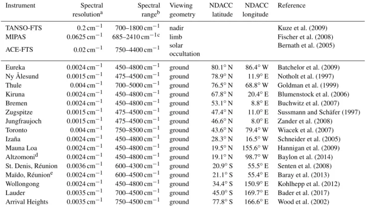
Table 1.FTS instruments used in the CH4VMR vertical profile comparisons presented herein.
Instrument Spectral Spectral Viewing NDACC NDACC Reference
resolutiona rangeb geometry latitude longitude
TANSO-FTS 0.2 cm−1 700–1800 cm−1 nadir Kuze et al. (2009)
MIPAS 0.0625 cm−1 685–2410 cm−1c limb Fischer et al. (2008)
ACE-FTS 0.02 cm−1 750–4400 cm−1 solar Bernath et al. (2005)
occultation
Eureka 0.0024 cm−1 450–4800 cm−1 ground 80.1◦N 86.4◦W Batchelor et al. (2009) Ny Ålesund 0.0015 cm−1 475–4500 cm−1 ground 78.9◦N 11.9◦E Notholt et al. (1997) Thule 0.004 cm−1 700–5000 cm−1 ground 76.5◦N 68.8◦W Goldman et al. (1999) Kiruna 0.0024 cm−1 450–4800 cm−1 ground 67.8◦N 20.4◦E Blumenstock et al. (2006) Bremen 0.0024 cm−1 450–4800 cm−1 ground 53.1◦N 8.8◦E Buchwitz et al. (2007) Zugspitze 0.0015 cm−1 475–4500 cm−1 ground 47.4◦N 11.0◦E Sussmann and Schäfer (1997) Jungfraujoch 0.0015 cm−1 475–4500 cm−1 ground 46.6◦N 8.0◦E Zander et al. (2008)
Toronto 0.004 cm−1 750–8500 cm−1 ground 43.6◦N 79.4◦W Wiacek et al. (2007) Izaña 0.0024 cm−1 450–4800 cm−1 ground 28.3◦N 16.5◦W Schneider et al. (2005) Mauna Loa 0.0024 cm−1 450–4800 cm−1 ground 19.5◦N 155.6◦W Hannigan et al. (2009) Altzomonid 0.0024 cm−1 450–4800 cm−1 ground 19.1◦N 98.7◦W Baylon et al. (2014) St. Denis, Réunion 0.0036 cm−1 600–4300 cm−1 ground 20.9◦S 55.5◦E Senten et al. (2008) Maïdo, Réunione 0.0024 cm−1 600–4500 cm−1 ground 21.1◦S 55.4◦E Baray et al. (2013) Wollongong 0.0024 cm−1 450–4800 cm−1 ground 34.4◦S 150.9◦E Kohlhepp et al. (2012) Lauder 0.0035 cm−1 700–4500 cm−1 ground 45.0◦S 169.7◦E Bader et al. (2017) Arrival Heights 0.0035 cm−1 750–4500 cm−1 ground 77.8◦S 166.6◦E Wood et al. (2002) aFor NDACC instruments, the best achievable spectral resolution is listed here. Operationally achieved spectral resolutions for NDACC instruments may be coarser. bNDACC instruments use optical filters that reduce the effective spectral range when making measurements.cMIPAS’ spectral resolution is divided into four narrower
bands.
dThe Altzomoni site came online in late 2012.eThe Maïdo, Réunion site came online in early 2013.
are computed over this range, and their correlations are ex-amined. Finally, this altitude range is used to estimate the mean VMR difference taken over the vertical range for each coincident pair of profiles. This data set shows any biases re-lated to latitude, or any other parameters of the TANSO-FTS retrieval, such as incidence angle or surface type (land or wa-ter).
Section 4 describes the methods and criteria for deter-mining coincident measurements between TANSO-FTS and each instrument. Section 6.1 provides a detailed descrip-tion of the comparison methodology. Comparison results for each instrument are presented in Sect. 6.2. The satellite in-struments are zonally averaged, and each NDACC site is shown. Partial column calculation methodology is presented in Sect. 7.1, and correlation results are shown in Sect. 7.2. A discussion follows in Sect. 8, focusing on our investigation of biases within the TANSO-FTS retrievals related to latitude and other parameters.
2 Data sets 2.1 TANSO-FTS
TANSO-FTS makes measurements of radiance in four bands; the TIR band is between 700 and 1800 cm−1and is used to
retrieve vertical profiles of CH4 VMRs. TANSO-FTS has
a spectral resolution of 0.2 cm−1 and operates in a
nadir-or near-nadir-viewing geometry (Kuze et al., 2009). To im-prove coverage, its field of view sweeps longitudinally, and TANSO-FTS makes several measurements along each cross track: five measurements prior to August 2010 and three since then (Kuze et al., 2012). This leads to TANSO-FTS having the highest density of measurements and greatest spa-tial coverage among the instruments considered herein.
Retrievals of v1 CH4follow the nonlinear maximum a
pos-teriori method used for v1 CO2 presented in Saitoh et al.
(2009, 2016). They are performed on a fixed pressure grid, and the pressure levels are adjusted based on the averaging kernels for the retrieval. In the v1 retrieval algorithm, wa-ter vapour, nitrous oxide, ozone concentrations, temperature, surface temperature, and surface emissivity were retrieved si-multaneously with CH4concentration from V161.160 L1B
spectra. A priori data are based on simulated data from the NIES transport model (TM; Maksyutov et al., 2008; Saeki et al., 2013), and the retrievals use the HITRAN 2008 line list (Rothman et al., 2009) with several updates up to 2011 (Saitoh et al., 2009).
An initial comparison of TANSO-FTS v1 to a single NDACC station, Eureka, and to ACE-FTS measurements made in the Arctic within a quadrangle surrounding PEARL
(60–90◦N and 120–40◦W) has been recently made (Holl
et al., 2016). The v1 CH4product was also compared
glob-ally with the version 6 CH4 data product from the
Atmo-spheric Infrared Sounder (AIRS) on Aqua (Zou et al., 2016). 2.2 ACE-FTS
ACE-FTS was launched into low Earth orbit in 2003 on board the Canadian Space Agency’s (CSA’s) SCISAT. The scientific objectives of ACE are to study ozone distribution in the stratosphere, the relationship between atmospheric chem-istry and climate change, the effects of biomass burning on the troposphere, and the effects of aerosols on the global en-ergy budget (Bernath, 2017).
ACE-FTS is a high-resolution, double-pendulum FTS with a spectral resolution of 0.02 cm−1that covers a broad spectral
range between 750 and 4400 cm−1. It operates in solar
oc-cultation mode, making a series of measurements for tangent altitudes down to 5 km (or cloud tops) at local sunrise and sunset along its orbital path (Bernath et al., 2005). Its Level 2 data products are vertical profiles of temperature, pressure, and the VMRs of 36 trace gases, as well as isotopologues of major species, reported on an altitude grid at the measure-ment tangent altitudes or interpolated onto a 1 km grid. Re-trievals of the version 2.2 (v2.2) data product are described in Boone et al. (2005), and updates regarding the latest re-lease, version 3.5 (v3.5), are described in Boone et al. (2013). V3.5 retrievals, with the data quality flags (v1.1) described in Sheese et al. (2015), are used herein.
When performing trace gas retrievals, tangent altitudes for each observation and vertical profiles of temperature and pressure are also retrieved using spectral fitting (not simul-taneously). Comparisons with TANSO-FTS are made on a pressure grid using the retrieved pressure values at the ACE-FTS measurement heights. A priori temperature and pressure for ACE-FTS are derived from the NRLMSISE-00 model (MSIS; Picone et al., 2002) and from meteorological data provided by the Canadian Meteorological Centre with their Global Environmental Multiscale (GEM) model (Côté et al., 1998). Fitted spectra are computed using the HITRAN 2004 spectral line list (Rothman et al., 2005) with modifications described in Boone et al. (2013).
Validation of v2.2 CH4VMR vertical profiles is presented
in de Mazière et al. (2008) and was performed using sev-eral ground-based FTSs that are part of NDACC, as well as one at Poker Flat. For that comparison, partial columns were computed from the ACE-FTS CH4 profiles, and the
correlation between partial columns computed from ground-based FTSs and from ACE-FTS was investigated. Validation was also done against the balloon-borne SPIRALE (Spec-troscopie Infra-Rouge d’Absorption par Lasers Embarqués), the Halogen Occultation Experiment (HALOE) on the Up-per Atmosphere Research Satellite, and MIPAS. de Maz-ière et al. (2008) determined that the ACE-FTS v2.2 CH4
data are accurate to within 10 % in the upper troposphere
and lower stratosphere and to within 25 % at high altitudes. More recently, Jin et al. (2009) compared CH4 from the
Canadian Middle Atmosphere Model (CMAM) with mea-surements from ACE-FTS, the Sub-Millimeter Radiometer (SMR) on Odin, and the Microwave Limb Sounder (MLS) on Aura, and they found agreement with ACE-FTS within 30 %. Updates to the ACE-FTS validation effort using v3.0 data and a description of the differences between v2.2 and v3.0 are presented in Waymark et al. (2013). Waymark et al. (2013) found a slight reduction in CH4VMR in the v3.0 data
near 23 km and a larger reduction of around 10% between 35 and 40 km.
2.3 MIPAS
MIPAS is a limb-sounding FTS that was placed in polar low Earth orbit in 2002 on board the European Space Agency’s (ESA’s) Envisat. MIPAS aimed to provide global observa-tions, during both night and day, of changes in the spatial and temporal distributions of long- and short-lived species, temperature, cloud parameters, and radiance. The instru-ment was intended to have a maximum spectral resolution of 0.025 cm−1(Fischer et al., 2008), but the slide system for the
interferometer mirrors encountered a problem in 2004, and observations used in this study were made with a reduced effective spectral resolution of 0.0625 cm−1 but with finer
vertical sampling. Further complications arose in 2012, and ESA lost communication with Envisat, ending the mission.
The spectral range of MIPAS is 685–2410 cm−1,
allow-ing the retrieval of multiple trace gases. MIPAS spectra are processed independently by four research groups (Raspollini et al., 2014). In this paper, we consider two: the ESA opera-tional analysis and the Karlsruhe Institute of Technology In-stitute of Meteorology and Climate Research (IMK) and the Instituto de Astrofísica de Andalucía (IAA) analysis, both described in the following subsections.
2.3.1 ESA MIPAS
We use MIPAS Level 2 Prototype Processor version 6 (ML2PP v6) of the ESA operational analysis. Early ver-sions of the ESA MIPAS gas retrievals are described in Raspollini et al. (2006) (full-resolution Instrument Process-ing Facility version 4.61; IPF v4.61), and the ML2PP v6 up-grades and reduced-resolution adaptations are described in Raspollini et al. (2013). Retrievals are made using a global fitting scheme followed by a posteriori Tikhonov regulariza-tion with self-adapting constraints (Raspollini et al., 2013). The ML2PP v6 data provide retrieved VMR vertical pro-files of 10 atmospheric gases between approximately 6 and 70 km. Temperature and pressure are retrieved from the spec-tra at each tangent point of a limb scan, and a correspond-ing altitude grid is built from the lowest engineercorrespond-ing tangent altitude using the equation of hydrostatic equilibrium. Ini-tial guesses for vertical profiles of a target trace gas,
tem-perature, and interfering species are the weighted average of the results from the previous scan, an appropriate merg-ing of IG2 (initial guess 2) climatological profiles (Remedios et al., 2007) and, if available, data from the European Centre for Medium-range Weather Forecasts (ECMWF). Spectra are computed using a specialized line list derived from HITRAN 1996 (Rothman et al., 1998).
The IPF v4.61 CH4 data product has been validated by
Payan et al. (2009) against four balloon instruments; includ-ing SPIRALE; three aircraft instruments; six ground-based FTSs (all are considered herein), and HALOE. They found good agreement with a 5 % positive bias in the lower strato-sphere and upper tropostrato-sphere. ML2PP v6 CH4 was
com-pared with BONBON air sampling measurements by En-gel et al. (2016). The reduced-resolution CH4measurements
(2005–2012) agree with in situ data within 5–10 %. CH4(and
N2O) from ESA MIPAS has been assimilated by the
BAS-COE code, and the assimilated products have been compared with MLS and ACE-FTS (Errera et al., 2016). The analysis has proven the high quality of the MIPAS data, but it has also identified the presence of some outliers, especially in the tropical lower stratosphere, and some discontinuities due to issues in the measurements.
2.3.2 IMK-IAA MIPAS
The IMK-IAA MIPAS retrieval algorithm has been devel-oped to include and account for deviations from local thermal equilibrium. The data presented here are IMK-IAA reduced-resolution version V5R_CH4_224/225. The early retrieval algorithms are described by von Clarmann et al. (2009), and the updates made to the current version are described by Plieninger et al. (2015). Temperature and tangent altitude are retrieved from the spectra, and pressure is computed from the equation of hydrostatic equilibrium. V5R_CH4_224/225 uses the HITRAN 2008 line list (Rothman et al., 2009). Tem-perature a priori profiles are determined from ECMWF anal-yses and MIPAS engineering information. The IMK-IAA re-trieval uses Tikhonov first-order regularization in combina-tion with an all-zero CH4 a priori profile, which serves to
smooth the profiles.
Validation of the IMK-IAA MIPAS V5R_CH4_222/223 data has been presented in Laeng et al. (2015). They compare data against ACE-FTS, HALOE, the MkIV balloon FTS, the Solar Occultation For Ice Experiment (SOFIE) on the Aeron-omy of Ice in the Mesosphere (AIM) satellite, the SCan-ning Imaging Absorption spectroMeter for Atmospheric CHartographY (SCIAMACHY) on Envisat, and a cryogenic whole-air sampler (collects gas bottle samples during aircraft flights). They found an agreement within 3 % in the upper stratosphere with other satellite instruments, but in the lower stratosphere (below 25 km) a high bias was found in the MI-PAS retrievals of up to 14 %. The V5R_CH4_224/225 has more recently been validated by Plieninger et al. (2016), us-ing ACE-FTS, HALOE, and SCIAMACHY. They found
MI-PAS CH4 retrievals to be larger by around 0.1 ppmv below
25 km, or around 5 %. 2.4 NDACC
NDACC is a global network of a variety of instruments that provides measurements of tropospheric and stratospheric gases that are directly self-comparable (Kurylo and Zander, 2000). The network consists of over 70 stations sparsely dis-tributed at all latitudes. Information about NDACC is avail-able at www.ndacc.org. In this work, we only consider a small subset of NDACC stations that feature high-resolution FTSs and provide a CH4 VMR vertical profile data
prod-uct via the NDACC database. Sepúlveda et al. (2012, 2014) demonstrated the good quality of CH4profiles that can be
retrieved from the NDACC FTS measurements. The stations are listed in Table 1, along with their locations, spectral range and resolution, and references.
The stations do not use identical instruments, spectro-scopic lines, or retrieval methods. All but one station use a version of a Bruker 120/5 M or HR and have predomi-nantly adopted, or upgraded to, the Bruker 125HR. Some sta-tions have more than one instrument, and the type of instru-ment has changed over time at many of the stations. Toronto, 43.6◦N, uses a Bomem DA8.
Retrievals are generally performed using either PROFFIT (Hase et al., 2004) or SFIT4 (Pougatchev et al., 1995) fol-lowing harmonized retrieval settings recommended by the NDACC IRWG (Sussmann et al., 2011, 2013). Data used herein are from the NDACC database. A summary of re-trieval settings is provided by Bader et al. (2017). Lauder and Arrival Heights, at 45.0 and 77.8◦S, respectively, use a
re-trieval strategy that adheres to that defined in Sussmann et al. (2011), with a relaxed Tikhonov regularization constraint at Arrival Heights due to the characteristic atmospheric dynam-ics over Antarctica. Jungfraujoch, at 46.6◦N, uses SFIT2. It
has been established within the NDACC IRWG that the reg-ularization strength of the CH4retrieval strategy should be
optimized so that the number of degrees of freedom for sig-nal (DOFS) is limited to approximately 2 (Sussmann et al., 2011).
3 Data set variability
To provide context for the VMR differences found when comparing each instrument to TANSO-FTS, shown in Sect. 6, we have examined the variability of retrievals made for each instrument. We are interested in determin-ing whether the mean differences found when compardetermin-ing TANSO-FTS to another instrument are comparable to the differences found when comparing pairs of retrievals for a single instrument. Each pair of observations compared in this study is made at different times and locations and subject to instrument noise and analysis errors. Examining the
variabil-ity within each data set provides an indication of the mag-nitude of these effects. Because the observation geometries and rates of spectral acquisition are different for each instru-ment, our internal comparisons differ for each instrument. For example, TANSO-FTS and MIPAS have a much higher data density than ACE-FTS, which only makes two sets of observations per orbit.
Following Holl et al. (2016), we are aware that TANSO-FTS CH4 retrievals are dependent on the a priori used,
es-pecially at high altitudes. TANSO-FTS vertical profiles tend to be similar to their a priori and, therefore, to each other. To provide context for our validation results, we computed the magnitude of the mean differences between the TANSO-FTS retrievals and their a priori. This is indicative of the in-strument sensitivity discussed in Sect. 5 and shows by how much the retrievals deviate from the a priori. We examined 3000 randomly selected TANSO-FTS measurements by in-terpolating the a priori and retrieved profiles to the pressure grid used in our comparisons (Sect. 6.1) and then computed the difference between the retrieval and the a priori at each pressure level, and their mean and standard deviation. Fig-ure 1 shows the mean ±1 standard deviation of the differ-ence between the TANSO-FTS CH4retrievals and their
cor-responding a priori profiles. The peak value is 30 ppbv near 10 km (∼ 1.5 %) with a standard deviation of the same mag-nitude.
To examine the variability of the ACE-FTS CH4 data
product, we compared each retrieved profile from an ACE-FTS sunset/sunrise (occultation direction) to that from the next orbit, taking care to avoid a comparison between sun-set and sunrise occultations (which are in different hemi-spheres), or when an acquisition was not recorded during a subsequent orbit. Considering all sunset occultations in 2011, there were 1402 retrieved vertical profiles,and 820 sequential pairs. These pairs are separated by 97 min and have a mean spatial separation of 1180 ± 20 km, depending on the lati-tude of the measurement. For each pair, we computed the VMR difference on the ACE-FTS 1 km tangent altitude grid and then found the mean and standard deviation, which are shown in Fig. 1. Within the ACE-FTS data, the largest sys-tematic variability (−4 ppbv) occurs around 30 km, with ex-treme outliers being observed at the lowest tangent altitudes. The mean magnitude of the ACE-FTS variability is 2 ppbv (0.1 %) at all altitudes and 9 ppbv below 15 km (0.4 %).
To examine the variability of the MIPAS data sets, we compared the vertical profiles retrieved by IMK-IAA and ESA that were made from the same MIPAS limb observa-tions and within our coincident data set. This provides an indication of the impact of different retrieval algorithms on retrieved profiles. For each pair of retrieved vertical profiles from a single set of MIPAS spectra, we interpolated the ESA retrieval to the IMK-IAA 1 km grid and computed their dif-ference (IMK-IAA − ESA), and then found the mean and standard deviation. Figure 1 shows the mean ±1 standard de-viation for this comparison. The two retrievals show good
−0.15 −0.10 −0.05 0.00 0.05 0.10 0.15 CH4VMR differences (ppmv) 101 102 Pressure (hP a) TANSO-FTS ACE-FTS MIPAS NDACC 5 10 15 20 25 30 Mean altitude (km)
Figure 1. Results for investigating the variability within each CH4VMR profile data set. Shown are the following comparisons: TANSO-FTS retrievals compared to their a priori (green), pairs of sequential ACE-FTS retrievals (red), ESA MIPAS retrievals com-pared to IMK-IAA MIPAS retrievals made for the same limb obser-vations (blue), and pairs of NDACC retrievals made on the same day (orange). All retrieved profiles used are coincident with TANSO-FTS. Dashed lines are 1 standard deviation.
agreement above 30 km (not shown), while the IMK-IAA data have a positive bias relative to the ESA data product of around 0.15 ppmv between 20 and 30 km. This bias is con-sistent with the validation results presented in Laeng et al. (2015). The ESA and IMK-IAA comparison exhibits the largest variability, with a mean magnitude (mean of abso-lute values) of 50 ppbv (2 %) for the altitude range consid-ered (9–34 km). Since the two products use the same spectra, it is possible that part of the internal instrument variability is hidden in this approach.
To investigate the variability of the NDACC data, we com-pared pairs of observations made at an NDACC site on the same day. We considered only NDACC CH4 VMR
verti-cal profiles that were in coincidence with TANSO-FTS. For each pair of NDACC measurements, we computed the CH4
VMR differences on the standard NDACC retrieval grid (ear-lier profile minus later profile; if there are multiple coinci-dences in a day, differences are found relative to the earli-est). The mean and standard deviation of these differences are also shown in Fig. 1. When examining several measurements from the same day, the NDACC differences show a system-atic mean increase in tropospheric CH4 with time during a
of −4 ppbv below 30 km and a peak at 12 km of −6 ppbv (0.3 %).
Our variability investigation found that the ACE-FTS data exhibit the smallest variability between measurements, that MIPAS exhibits the largest, and that NDACC and TANSO-FTS are of similar magnitudes. The magnitude of the in-ternal variability of the data sets is between ±2 ppbv (e.g., for NDACC and ACE-FTS in the upper troposphere) and ±3 ppbv, or around 2 % (e.g., for TANSO-FTS and the lower limits of ACE-FTS).
4 Coincidences
Due the coverage and data collection rates of each instru-ment, different coincidence criteria were used. ACE-FTS has an inclination of 74◦ and operates in solar occultation
mode, recording only two occultations per orbit, predomi-nantly at high latitudes; the NDACC sites are stationary; MI-PAS makes frequent observations at all latitudes; and the spa-tial distribution of TANSO-FTS observations is enhanced by its cross-track observation mode. In the case of ACE-FTS and NDACC stations, the objective of the coincidence crite-ria was to maximize the number of measurements used. Con-versely, in the case of MIPAS, the objective was to reduce the number of potential coincident measurements. For ACE-FTS and NDACC, we sought measurements made within 12 h and within 500 km of each TANSO-FTS measurement (spatial separation calculated using the Vincenty method (Vincenty, 1975)). For the MIPAS data sets, we sought measurements made within 3 h and 300 km. When searching for MIPAS– TANSO-FTS coincidences within 12 h and 500 km, we find approximately 180 000 coincidences per month.
The criteria used in this study are comparable to previous CH4studies. For example, de Mazière et al. (2008) used
cri-teria of 24 h and 1000 km when comparing ACE-FTS CH4to
ground sites, and 6 h and 300 km when comparing ACE-FTS to MIPAS. Payan et al. (2009) used criteria of 3 h and 300 km when comparing MIPAS CH4to ground- and satellite-based
spectrometers. Laeng et al. (2015) used criteria of 9 h and 800 km when comparing MIPAS CH4to ACE-FTS, and 24 h
and 1000 km when comparing MIPAS to HALOE.
TANSO-FTS CH4 VMR vertical profiles tend not to be
sensitive above the upper troposphere (see Sect. 5), while ACE-FTS and MIPAS retrievals have a limited vertical ex-tent in the troposphere. To ensure that measurements made by each instrument overlap, a restriction was placed on ACE-FTS and MIPAS measurements: that their retrieved vertical profiles extend to low enough altitudes, after applying data quality criteria. For ACE-FTS, this requirement was 10 km. For MIPAS, this requirement was relaxed to less than 12 km. IMK-IAA MIPAS CH4VMR vertical profile retrievals do not
extend as low as those made by ESA, to the extent that hav-ing the same restriction on altitude range results in only a quarter as many coincidences as the ESA data product.
Re-laxing the constraint to only 12 km maintains the assurance that retrieved VMRs will overlap with the TANSO-FTS al-titude range, though there are only 60 % as many IMK-IAA coincidences as ESA coincidences.
TANSO-FTS makes nadir observations in a grid pattern by sweeping its line of sight across its ground-track. This re-sults in a high density of vertical profiles, such that – for a single observation made by ACE-FTS, MIPAS, or NDACC – there are an average of 11 coincident TANSO-FTS mea-surements. The subsequent measurement made by MIPAS or an NDACC station will be coincident with a similar number of TANSO-FTS measurements, and most of those will also be coincident with the previous MIPAS or NDACC measure-ment. A common way to deal with multiple coincidences is to take the mean of the VMR vertical profiles from each in-strument and to compute the difference of the means (e.g., Holl et al., 2016). When comparing MIPAS to TANSO-FTS, however, this results in some measurements contributing to the analysis more times than others, biasing the computed VMR difference profiles. Furthermore, this leads to using a mean TANSO-FTS VMR vertical profile that is strongly smoothed, while a coincident ACE-FTS (or NDACC, de-pending on the station’s rate of acquisition at the time) VMR vertical profile is not.
To reduce biases caused by over-counting, when compar-ing TANSO-FTS to MIPAS, and by smoothcompar-ing, when com-paring TANSO-FTS to ACE-FTS, we reduced the number of coincident measurements by seeking a set of one-to-one coincidences for unique measurements in the sparser data set (which is always ACE-FTS, MIPAS, or NDACC). For each measurement that is being compared to TANSO-FTS, we find the TANSO-FTS measurement with the minimum of the sum of ratios of distance in space and time to the co-incidence criteria, giving equal weight to both parameters as min(dx/xcrit+dt/tcrit), where dx and dt are the distance and time between a given measurement and a TANSO-FTS coincidence, and xcrit and tcrit are the coincidence criteria.
This method is similar to using a standard score to compare the spatial and temporal separation, but the sample size of the set of TANSO-FTS measurements coincident with an-other measurement is on the order of only 10. Furthermore, the mean and standard deviations of dx and dt reflect the time and distance between each consecutive TANSO-FTS measurement, rather than the time and spatial separation be-tween each TANSO-FTS measurement and those from MI-PAS, ACE-FTS, or NDACC.
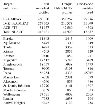
Table 2 shows the total number of coincidences found be-tween TANSO-FTS and each validation target instrument, as well as the subsets of unique TANSO-FTS measurements and the one-to-one coincidences used in this paper (equiv-alent to the number of unique measurements made by each target instrument). Figure 2 shows an example of the global distribution of coincident measurements. Shown are the first 200 one-to-one coincidences after 1 January 2012. For the ESA and IMK-IAA MIPAS data products, this number of
Table 2.Number of coincident CH4VMR vertical profile measure-ments that were found between TANSO-FTS retrievals and those from ESA MIPAS, IMK-IAA MIPAS, ACE-FTS, and NDACC sta-tions. The three columns show the total number of coincidences found, the number of unique TANSO-FTS measurements within those coincidences, and the size of the reduced one-to-one coin-cidences used.
Target Total Unique One-to-one
instrument coincident TANSO-FTS profiles
profiles profiles used
ESA MIPAS 450 230 358 267 85 386 IMK-IAA MIPAS 267 065 210 573 51 099 ACE-FTS 51 937 47 560 4302 Total NDACC 213 181 44 920 17 637 Eureka 11 843 2447 1009 Ny Ålesund 5445 1300 349 Thule 6997 3359 513 Kiruna 4595 2056 529 Bremen 2610 1452 211 Zugspitze 47 512 5743 3469 Jungfraujoch 18 757 5938 1493 Toronto 9909 5195 816 Izaña 56 254 4336 4501∗ Mauna Loa 4338 2381 379 Altzomoni 4746 854 486 St. Denis, Réunion 12 270 3161 1507 Maïdo, Réunion 3139 868 383 Wollongong 27 781 4808 2365 Lauder 7083 2638 704 Arrival Heights 5042 3122 258
∗The Izaña NDACC coincidence data set is the only one in which TANSO-FTS
measurements are more sparse. For consistency, Izaña was not treated as a special case.
coincidences is found in around 2 weeks. For ACE-FTS and the NDACC stations (combined), these coincidences occur over several months.
5 Averaging kernels
The averaging kernels of a profile retrieval provide informa-tion about the contribuinforma-tions of the retrieval from a priori in-formation and the measurements. In this study, the retrieval methods for each data set differ, and the averaging kernel ma-trices are differently defined. In general, the rows of the av-eraging kernel matrix are peaked functions whose full width at half maximum (FWHM) can be used to define the vertical resolution of the measurement. The sum of the rows of the matrix gives the sensitivity, or response, of the retrieval. A sensitivity close to 1 indicates that most of the information in the retrieval comes from the measurement, while sensitivities less than 1 indicate increased reliance on the a priori in the solution.
The rows of the averaging kernel matrices for the ESA MIPAS, IMK-IAA MIPAS, TANSO-FTS, and the Eureka NDACC station are shown in Fig. 3. Each panel shows the mean from 30 retrievals. Vertical profiles of pressure
associ-ated with each retrieval’s averaging kernel matrix are, in gen-eral, unique, so a common pressure grid was selected for each instrument, and averaging kernels were interpolated prior to averaging.
In this study, we treat TANSO-FTS retrievals as having the coarser vertical resolution in all cases, despite the widths of the kernel functions shown in Fig. 3a, which are comparable to MIPAS and narrower than NDACC. The peak locations of the TANSO-FTS averaging kernels do not match the corre-sponding pressure level of each kernel. Therefore the FWHM values when considering the location of the appropriate pres-sure level are much larger than the FWHM values for the averaging kernels of the other instruments.
In the NDACC retrievals, the a priori has a large role, and information coming from the measurements can hardly dis-tinguish the contribution coming from the different altitudes. This leads to wide, overlapping averaging kernels. The IMK-IAA MIPAS retrievals use a form of Tikhonov regulariza-tion without an a priori. The ESA MIPAS retrievals use the regularizing Levenberg–Marquardt approach (where the pa-rameter setting has been chosen to leave results largely in-dependent from the initial-guess profiles) and a posteriori Tikhonov regularization without an a priori. The ACE-FTS retrievals do not use a regularized matrix inverse method. Consequently, the ACE-FTS and IMK-IAA MIPAS averag-ing kernels are very narrow, their peak values are close to 1 at each altitude where a spectrum was acquired, and the solutions do not rely on a priori information. Very similar averaging kernel are obtained also for ESA MIPAS, with wider widths at lower altitudes where the retrieval grid used is coarser than the measurement grid. The sensitivity of both ACE-FTS and MIPAS, shown in Fig. 3e, is close to 1 at all altitudes, falling off above 60 or 70 km. ACE-FTS averag-ing kernels are under development, and preliminary work is shown in Sheese et al. (2016).
The typical sensitivity of an NDACC retrieval is close to unity until above 20 km, falling off towards 0 through 60 km. The sensitivity of TANSO-FTS only reaches 0.2–0.3 between 5 and 10 km. The implication of such low values for sensitivity is that the TANSO-FTS retrievals are highly dependant on their a priori.
The trace of the averaging kernel matrix gives the DOFS. For example, DOFS for retrievals made by TANSO-FTS, IMK-IAA MIPAS, ESA MIPAS, and NDACC from obser-vations over the Arctic, above 60◦N, are shown in Fig. 4.
The IMK-IAA MIPAS and TANSO-FTS data are in coinci-dence with one another. The NDACC data come from Eu-reka, Ny Ålesund, and Thule. The NDACC and ESA MI-PAS data shown are the TANSO-FTS one-to-one coinci-dences used throughout this study (but are not coincident with the TANSO-FTS data shown in the top panel of Fig. 4). The trends visible are seasonal and are related to opacity and water vapour content. Recreating this figure over mid-latitudes or the tropics reveals a flat trend over time, while over Antarctica the trends are reversed in DOFS space.
80◦S 60◦S 40◦S 20◦S 0◦ 20◦N 40◦N 60◦N 80◦N 120◦W 60◦W 0◦ 60◦E 120◦E TANSO-FTS ACE-FTS IMK-IAA MIPAS ESA MIPAS NDACC
Figure 2.Locations of the first 200 observations of 2012 used in this study for TANSO-FTS (green), ACE-FTS (red), IMK-IAA MIPAS (blue), and ESA MIPAS (purple). The NDACC stations are shown in orange.
0.000 0.015 0.030 TANSO-FTS 101 102 Pressure (hP a) (a) 870.7 hPa 502.5 hPa 216.5 hPa 63.0 hPa 7.8 hPa 0.0 0.2 0.4 IMK-IAA MIPAS (b) 461.1 hPa 190.9 hPa 73.2 hPa 33.0 hPa 15.2 hPa 0.0 0.3 0.6 ESA MIPAS (c) 222.3 hPa 110.9 hPa 54.7 hPa 34.2 hPa 0.00 0.05 0.10 Eureka NDACC (d) 734.7 hPa 288.2 hPa 66.7 hPa 9.0 hPa 0.3 hPa 0.0 0.5 1.0 1.5 Sensitivity (e) 5 10 15 20 25 30 Mean altitude (km)
Figure 3.Example of averaging kernels for (a) TANSO-FTS, (b) IMK-IAA MIPAS, (c) ESA MIPAS, and (d) NDACC. Each kernel shown is the mean from 30 averaging kernel matrices from measurements made over the Arctic, interpolated to a common pressure grid. Panel (d)shows the mean averaging kernels from the Eureka station. Panel (e) shows the sensitivity for the mean averaging kernels shown in each panel: TANSO-FTS (green), IMK-IAA MIPAS (blue), ESA MIPAS (purple), and NDACC (orange).
The mean of the DOFS for the three NDACC stations over the Arctic is 1.98 with a standard deviation, σ , of 0.50. Over the tropics, considering data from Izaña, Réunion St. De-nis, Altzomoni, and Mauna Loa (Réunion Maïdo only has data from 2013 onward, not shown here), the mean is 2.39 with σ = 0.37. The mean DOFS for IMK-IAA MIPAS are slightly larger than those for ESA MIPAS. Over the Arctic,
their means and standard deviations are 17.05 and σ = 1.06 for IMK-IAA, and 15.76 and σ = 0.93 for and ESA, respec-tively. Over the tropics, they are 16.10 and σ = 0.33, and 15.88 and σ = 1.20.
The TANSO-FTS DOFS are larger at low latitudes, with a mean over the tropics of 0.72 and σ = 0.08, and means over the Arctic and Antarctic of 0.32 and 0.20, respectively
0.0 0.2 0.4 0.6 0.8 TANSO-FTS 2010 2011 2012 14 15 16 17 18 19 20 IMK MIP AS 2010 2011 2012 8 10 12 14 16 18 20 ESA MIP AS 2010 2011 2012
Feb Mar Apr May Jun Jul Aug Sep Oct Nov Dec
Month of year 0.5 1.0 1.5 2.0 2.5 3.0 3.5 4.0 ND A CC 2010 2011 2012
Figure 4.Degrees of freedom for signal for, from top to bottom, TANSO-FTS, IMK-IAA MIPAS, ESA MIPAS, and NDACC. Each satellite (and panel) uses a different symbol and colour, but the colour shades indicate the year the measurement was made in. The TANSO-FTS and IMK-IAA MIPAS measurements shown are in coincidence. The ESA MIPAS and NDACC data are from our analyzed data set but not in coincidence with the TANSO-FTS data in the top panel. All data are from the Arctic, 90–60◦N, with the NDACC measurements from Eureka, Ny Ålesund, and Thule.
(σ = 0.13 and 0.12). The DOFS for a TANSO-FTS retrieval rarely go above unity. Conversely, in the coincident NDACC data discussed above, over the tropics and Arctic, the DOFS never fall below unity. Note that the averaging kernel matri-ces for TANSO-FTS, and therefore the DOFS, cover a much smaller altitude range than for NDACC and MIPAS, which can extend above 100 km.
6 VMR vertical profile comparisons 6.1 Methodology
Retrievals made by an instrument with fine vertical resolution may result in structure over its vertical range that is not dis-tinguishable in retrievals made by an instrument with coarser vertical resolution. In order to make the best comparison be-tween two instruments with differing vertical resolution, it is necessary to smooth the vertical profiles retrieved from the finer-resolution instrument, in order to simulate what we could infer from it if it had a sensitivity similar to that of the other instrument. Smoothing is done using the a priori CH4
VMR vertical profiles and averaging kernel matrices of the instrument with lower vertical resolution (Rodgers and Con-nor, 2003):
ˆ
xs=xa+A( ˆx − xa), (1)
where ˆx is original higher-resolution retrieved profile, ˆxs is
the smoothed profile, xais the a priori profile of the
lower-resolution retrieval, and A is the averaging kernel matrix of
the lower-resolution retrieval. xaand A are from the
TANSO-FTS retrieval in all cases presented here. The smoothed pro-file, ˆxs, approximates the a priori, xa, when either the rows
of A are close to 0, or when the retrieval is close to xa. As
can be inferred from Fig. 3a, above 20–25 km ˆxs∼xa. In order to apply Eq. (1), all the variables on the right-hand side must be interpolated to a common grid. TANSO-FTS retrievals are done on a retrieved pressure grid. Determining the altitude of its VMR vertical profiles requires applying the equation of hydrostatic equilibrium and incorporating a pri-ori temperature and water vapour. Since pressure is retrieved by ACE-FTS and MIPAS, and the tropospheric a priori pres-sure profiles and meapres-sured surface prespres-sure are accurate for NDACC (Sepúlveda et al., 2014), all comparisons here have been done on a common pressure grid, as opposed to an alti-tude grid.
The data products do not always overlap over the entire pressure range of the common grid. Extrapolation is needed to ensure that the length of ˆx matches the dimensions of A in Eq. (1). For ACE-FTS and MIPAS, we use xato extend their
retrieved profiles below their altitude range to cover the full pressure range of the TANSO-FTS averaging kernels. The averaging kernels at these non-overlapping pressure levels do not contribute to the smoothed retrieval at higher, overlap-ping levels. The following steps are taken to compute vertical profiles of the mean CH4VMR differences:
1. appropriate instrument data quality flags are applied to each VMR vertical profile in the coincidence pair;
2. TANSO-FTS a priori and validation target VMR verti-cal profiles are interpolated to the TANSO-FTS retrieval pressure grid;
3. the interpolated validation target profile is extended as needed to match the TANSO-FTS pressure range (and vector length) using the TANSO-FTS a priori;
4. the interpolated validation target profile is smoothed using the TANSO-FTS averaging kernel matrix using Eq. (1);
5. TANSO-FTS-retrieved and validation-target-smoothed VMR vertical profiles are interpolated to a standard pressure grid, and levels outside the pressure range of the target’s VMR profile are discarded;
6. the piecewise difference between the TANSO-FTS and the smoothed validation target VMR vertical profiles is found;
7. the means, standard deviations, and correlation coeffi-cients of the VMR differences are calculated at each level of the standard pressure grid for all coincidences within a latitude zone.
For comparison, mean VMR vertical profile differences were also computed without smoothing by using only steps 1, 5, 6, and 7. Zonally averaged VMR difference pro-files are presented in Sect. 6.2, and results obtained with-out applying smoothing to the validation targets are shown in Sect. 6.3. The data quality flags in step 1, referring to variables in the data product files, were, for TANSO-FTS, CH4ProfileQualityFlag must be 0; for ACE-TANSO-FTS, qual-ity_flag must be 0 and cannot be equal to 4, 5, or 6 at any alti-tude; for ESA MIPAS, ch4_vmr_validity must be 1, and pres-sure_error cannot be NaN (not a number); and for IMK MI-PAS, visibility must be 1, and akm_diagonal must be greater than 0.03.
Holl et al. (2016) found that identifying and removing co-incident CH4VMR vertical profile pairs that may have one
or both profile locations within a polar vortex, and then fil-tering these events, had little effect on their vertical profile comparisons below 25 km. Polar vortex event will have a much smaller effect on this study since it uses global and year-round data sets. For these two reasons, our method does not filter for profiles located within a polar vortex. Ar-rival Heights may be differently affected by a much stronger Antarctic polar vortex, but comparison results from this site are not anomalous and only account for 1.5 % of the NDACC data set, so they are treated in a consistent manner.
6.2 Zonally averaged VMR profile differences
Following Holl et al. (2016), we are trying to determine whether there are any zonal biases in the TANSO-FTS data or zonal dependencies when making comparisons to other
instruments. The mean CH4 VMR differences, averaged
zonally, between the TANSO-FTS vertical profiles and the smoothed vertical profiles from ACE-FTS, IMK-IAA MI-PAS, ESA MIMI-PAS, and each NDACC station are show in Fig. 5. Each row in Fig. 5 shows the results from five latitudi-nal zones: 90–60◦N, 60–30◦N, 30◦N–30◦S, 30–60◦S, and
60–90◦S. The left-most column shows the mean differences
between the retrievals from TANSO-FTS and those from the other instruments, always calculated as TANSO-FTS minus target. One standard deviation is shown for each instrument comparison with dotted lines. The middle-left column shows the mean differences as a percentage of the mean CH4VMR
vertical profile taken for the target validation instrument in each zone. The number of VMR measurements used in the mean at each altitude, for each comparison, is shown in the right-most panel, with ESA MIPAS always having the most. At each altitude, we also calculated the Pearson correlation coefficient between the set of TANSO-FTS CH4VMR
mea-surements and the coincident set from each validation instru-ment. These are shown in the middle-right column for each panel in Fig. 5.
For each zone, the mean difference tends towards 0, and the standard deviation falls off above 100 hPa. This is a re-flection of the TANSO-FTS sensitivity. Above this altitude, the TANSO-FTS averaging kernels tend to 0, as shown in Fig. 3, and the smoothed profiles from each target instru-ment begin to approximate the TANSO-FTS a priori. Like-wise, the TANSO-FTS retrieval above this pressure level is also close to its a priori. Conversely, the number of CH4
VMR measurements in the mean falls off sharply below 10– 12 km, or around 80–90 hPa, for the comparisons to the satel-lite instruments. For the satelsatel-lite instruments and many of the NDACC stations we see the same trend: a positive bias (TANSO-FTS VMRs are greater than those of the valida-tion instruments) decreasing with increasing altitude, with a tropospheric mean of around 20 ppbv, or 1 %. The bias is smallest for the two MIPAS data products in the tropics, be-tween 30◦N and 30◦S. The bias relative to ACE-FTS is
con-sistent in all the zones. For three of the NDACC stations – Ny Ålesund, Bremen, and Toronto – there is a negative bias (TANSO-FTS retrieves less CH4than these stations), and for
Eureka and Jungfraujoch the bias is close to 0.
There is a notable feature just below 100 hPa in all the zones except 30–60◦S. This feature is a pronounced increase
in the mean difference in the northern zones 60–30◦N and
90–60◦N, while it is a decrease in the mean difference
be-tween 30◦N and 30◦S and between 60 and 90◦S. It is around
this pressure level, or altitude, that the VMR of CH4
be-gins to fall off rapidly from between 1.8 and 2 ppmv in the troposphere towards 0 ppmv in the upper stratosphere and mesosphere. This feature indicates that the altitude at which this VMR decrease occurs differs between instruments. In the Northern Hemisphere this decrease in CH4 VMR
oc-curs at higher altitudes for TANSO-FTS than for the other instruments, and in the tropics and Southern Hemisphere
−40 −20 0 20 40 60 102 Pressure (hP a) 90–60◦N −3 −2 −1 0 1 2 3 4 0.00 0.25 0.50 0.75 1.00 Eureka Kiruna Ny Alesund Thule 0 10000 20000 5 10 15 20 25 Mean altitude (km) −40 −20 0 20 40 60 102 Pressure (hP a) 60–30◦N −3 −2 −1 0 1 2 3 4 0.00 0.25 0.50 0.75 1.00 Bremen Jungfraujoch Toronto Zugspitze 0 6000 12000 180005 10 15 20 25 Mean altitude (km) −40 −20 0 20 40 60 102 Pressure (hP a) 30◦N to 30◦S −3 −2 −1 0 1 2 3 4 0.00 0.25 0.50 0.75 1.00 Réunion St. Denis Réunion Maïdo Altzomoni Mauna Loa Izana 0 4000 8000 120005 10 15 20 25 Mean altitude (km) −40 −20 0 20 40 60 102 Pressure (hP a) 30–60◦S −3 −2 −1 0 1 2 3 4 0.00 0.25 0.50 0.75 1.00 Lauder Wollongong 0 5000 10000 5 10 15 20 25 Mean altitude (km) −40 −20 0 20 40 60 ∆ CH4VMR (ppbv) 102 Pressure (hP a) 60–90◦S −3 −2 −1 0 1 2 3 4 CH4VMR rel. diff. (%) 0.00 0.25 0.50 0.75 1.00 Correlation coefficient Arrival heights 0 10000 20000 No. coincidences 5 10 15 20 25 Mean altitude (km) 0.0 0.2 0.4 0.6 0.8 1.0
ACE-FTS IMK-IAA MIPAS ESA MIPAS
Figure 5.Zonally averaged comparison results. The rows present results for each zone, from top to bottom: 90–60◦N, 60–30◦N, 30◦N– 30◦S, 30–60◦S, and 60–90◦S. In each row, the four panels show, from left to right, the mean CH
4VMR difference between retrievals from TANSO-FTS and the validation target at each pressure level; the mean CH4VMR differences relative to the mean CH4VMR vertical profile of the validation target; the correlation coefficients R2of the CH4VMR differences for each coincident pair at each pressure level; and the number of coincidences at each pressure level. Differences are calculated as TANSO-FTS minus target for each data set compared. In all frames, ACE-FTS is shown in red, ESA MIPAS is purple, IMK-IAA MIPAS is blue, and NDACC stations are shades of orange. Each individual NDACC station with a zone is shown, and their shades indicated.
this decrease occurs more rapidly and at lower altitudes for TANSO-FTS.
For all instruments and in all zones, the correlation coef-ficients, R2, at each altitude fall off very sharply, to around
0.2, below the 90 hPa level (and remain higher in the trop-ics). This indicates that biases seen in the mean differences are not uniform across the coincident data set and that there is significant variability in the magnitudes of the differences
for individual vertical profile pairs and in the direction of the difference. This is related not only to the increasing standard deviation of the differences with decreasing altitude but also to the standard deviations of each data product in the com-parison. The sharpness and altitude of the decrease are di-rectly related to the TANSO-FTS averaging kernels. Above the 100 hPa level, the standard deviations of the TANSO-FTS and the smoothed validation target fall off very sharply as they both begin to approximate the a priori (which also ex-plains why R2is close to 1).
6.3 Impact of smoothing
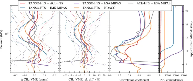
This study was also performed without applying any smooth-ing to the vertical profiles of the target validation instruments. These results are shown in Fig. 6, which has the same panels as Fig. 5. The data have not been separated zonally, and the plots show means for all latitudes. No zonal biases were ob-served in the unsmoothed data. The 16 NDACC stations have been combined into a single data set.
Figure 6 shows the mean differences between the TANSO-FTS data product and those of other instruments, and the behaviour of the comparisons at higher altitudes when the validation targets are unaffected by the TANSO-FTS aver-aging kernels. Without the smoothing applied, the difference profiles in Fig. 6 show more consistent behaviour over the pressure, or altitude, range shown. While the magnitude of the differences is much greater without smoothing, it is not consistently biased high or low for all the data products at all altitudes. When comparing to the satellite instruments in the upper troposphere, we find that the TANSO-FTS retrieval has greater CH4VMRs by around 50 ppbv, or around 3 %.
For context, a comparison between the ACE-FTS and ESA MIPAS data products, using profiles that were coincident with the same TANSO-FTS observation, is shown in grey. The mean differences between these two data products are smaller than those relative to TANSO-FTS but have compa-rable standard deviations and a slightly smaller correlation, with R2=0.5 and 0.6 in the upper troposphere.
The comparison between TANSO-FTS and NDACC ex-tends below the range of ACE-FTS and MIPAS. NDACC and TANSO-FTS agree very well in this region, between ±30 ppbv, or between ±2 %. In this case, the NDACC stations retrieve more CH4, on average. The low-altitude
NDACC and TANSO-FTS data are also more closely linearly correlated, between 50 and 60 %. It should also be noted that the standard deviation of the TANSO-FTS and NDACC dif-ferences is also less than those for ACE-FTS and MIPAS at all altitudes.
7 Partial column comparisons 7.1 Methodology
For each CH4 VMR vertical profile in a pair of coincident
measurements, we computed a partial column and compared those from TANSO-FTS to each of the other instruments to investigate how well correlated the derived CH4abundances
are. For consistency, each pair of partial columns must be calculated over the same pressure range, as the number of molecules in the column strongly depends on the altitude range (length of the column) of the integral. To determine the pressure range over which to compute partial columns for each coincident pair of profiles, we considered the TANSO-FTS averaging kernels.
We investigated the sensitivity of the TANSO-FTS re-trievals, as defined in Sect. 5 to find an altitude range which minimizes the partial column dependence on a pri-ori information, ensuring our investigation is focused on re-trieved information from TANSO-FTS. Figure 7 shows a two-dimensional histogram of the number of TANSO-FTS profiles, for all validation targets combined for two criteria: setting a requirement that the sensitivity must be greater than some threshold and the resulting number of usable pressure levels in the integral for each profile. We see that the max-imum number of usable levels falls off in an approximately linear manner with increasing sensitivity threshold, and that for any sensitivity threshold there will be a large number of TANSO-FTS CH4VMR vertical profiles that never meet the
sensitivity criteria. Increasing the sensitivity cutoff by 0.05 causes approximately 10 000 additional TANSO-FTS verti-cal profiles, or around 6 % of the total data set combining all validation targets, to fail to meet the requirement at any alti-tude. The number of usable pressure levels given a restriction on sensitivity is not normally distributed, as can be inferred from the empty area in the upper right of Fig. 7.
For this study, we have selected a sensitivity threshold of 0.2 and require a minimum of three integrable pressure lev-els. Approximately 23 % of the TANSO-FTS retrievals do not meet these criteria. In such a case, partial columns are still computed using three pressure levels surrounding the level with the maximum sensitivity that are within the range of the target profile (e.g., not below 10 km when comparing to ACE-FTS). These excluded data do not exhibit a broader distribution, but their computed partial columns are all very small due to the integration range. Because the overlapping altitude regions for NDACC and TANSO-FTS measurements extend much lower in the atmosphere than for ACE-FTS and MIPAS, the number of TANSO-FTS profiles that do not meet the sensitivity criteria is much smaller for NDACC.
Partial columns are computed as
column = z2 Z z1 P (z) kT (z)χ (z)dz, (2)
−0.2 −0.1 0.0 0.1 0.2 ∆ CH4VMR (ppmv) 102 Pressure (hP a) −20 −15 −10 −5 0 5 10 15 20 CH4VMR rel. diff. (%) 0 30000 60000 90000 No. coincidences 5 10 15 20 25 Approximate Altitude (km) 0.0 0.2 0.4 0.6 0.8 1.0 Correlation coefficient TANSO-FTS − ACE-FTS
TANSO-FTS − IMK MIPAS
TANSO-FTS − ESA MIPAS TANSO-FTS − NDACC
ACE-FTS − ESA MIPAS
Figure 6.Averaged comparison results, as in each panel of Fig. 5, for all latitudes, without applying smoothing to the validation instruments’ CH4VMR vertical profiles. Differences are calculated as TANSO-FTS minus target for each data set compared (and ACE-FTS-ESA MIPAS for that case).
0.1 0.2 0.3 0.4 0.5 Sensitivity threshold s 0 5 10 15 Number of usable TANSO-FTS le vels 101 102 103 104 Number of TANSO-FTS profiles
Figure 7. Two-dimensional histogram showing the number of TANSO-FTS CH4VMR profiles within our data set (z axis) that have some number of usable pressure levels (y axis) with a sen-sitivity greater than some given threshold, s (x axis). The data set shown here consists of all TANSO-FTS observations that are one-to-one coincident with a target validation data set. The threshold chosen for this study was s = 0.2.
where z1and z2bound the integration range over altitude z,
P is pressure, T is temperature, χ is the CH4VMR, and k is the Boltzmann constant. For each instrument, χ(z) is the
retrieved quantity, and either retrievals were performed on a pressure grid or pressure was retrieved simultaneously. We compute partial columns from vertical profiles after step 5 in Sect. 6.1, so both the TANSO-FTS and the smoothed val-idation target profiles have the same pressure at each level in the integration. Since TANSO-FTS retrievals do not have an altitude grid, we use that of the coincident measurement, which corresponds to the pressure levels and should be very accurate within the altitude range considered in this study (upper troposphere to lower stratosphere). Thus, we are in-tegrating over the same altitude range for both instruments. Since ACE-FTS and both MIPAS data products include re-trieved temperatures, we use their rere-trieved temperature. For TANSO-FTS and NDACC, we use their corresponding a pri-ori temperatures.
Several methods of integration were investigated, and the results presented in Sect. 7.2 are derived by simple summa-tion of the integrand multiplied by the bin width of each data point in kilometers. We also used numerical integration tech-niques, variations of Newton–Cotes and Gaussian quadrature formulas. These did not provide significantly different results due the large size of our sample (i.e., our results are statistics found from the least-squares method, and small differences in the individual partial columns due to different integration methods do not introduce bias). Since the analytic function being integrated is not well defined, neither is the uncertainty of the derived partial column. Propagating reported retrieval uncertainties of temperature and VMR provides the most ap-propriate estimate of uncertainty, which is shown in Fig. 8.
7.2 Partial column correlation
The computed partial columns from TANSO-FTS are plotted against those from each validation instrument in Fig. 8. The
0.2 0.4 0.6 0.8 1.0 1.2 1.4 1.6 1.8 2.0 ACE-FTS PC (molec. cm )– 2 0.4 0.8 1.2 1.6 2.0 TA N SO -F T S PC ×1024 ×1024 y = mx + b m = 1.011 ± 0.001 b = 1.8e+21 ± 1.0e+21 R2= 0.9986 0.3 0.4 0.5 0.6 0.7 0.8 0.9 1.0 IMK MIPAS PC 0.3 0.4 0.5 0.6 0.7 0.8 0.9 1.0 ×1024 y = mx + b m = 1.001 ± 0.002 b = 2.6e+21 ± 7.7e+20 R2= 0.9965 ×10²³ 0.2 0.4 0.6 0.8 1.0 1.2 1.4 1.6 1.8 2.0 ESA MIPAS PC 0.4 0.8 1.2 1.6 2.0 ×1024 ×1024 y = mx + b m = 0.989 ± 0.000 b = 1.0e+22 ± 2.4e+20 R2= 0.9968 0.5 1.0 1.5 2.0 2.5 3.0 3.5 4.0 NDACC PC 0.5 1.0 1.5 2.0 2.5 3.0 3.5 4.0 ×1024 ×1024 y = mx + b m = 0.989 ± 0.001 b = 2.6e+22 ± 1.6e+21 R2= 0.9958
(molec. cm )– 2 (molec. cm )– 2 (molec. cm )– 2
(m ol ec . c m ) – 2
Figure 8.Partial column (PC) correlation plots comparing TANSO-FTS CH4to each validation instrument. Comparisons to ACE-FTS are red, to IMK-IAA MIPAS are blue, to ESA MIPAS are purple, and to NDACC are orange. The vertical range of partial column integration varies for each pair of coincident profiles based on the criteria described in Sect. 7.1. The statistics for weighted linear least-squares regression are shown, with weights equal to 1/(δx2+δy2).
panels for ACE-FTS, ESA MIPAS, and IMK-IAA MIPAS contain measurements for all latitudes, and that for NDACC combines results from all 16 stations. Since IMK-IAA re-trievals do not extend as low as those of ESA generally, the altitude range of the partial column integral is often smaller than those of the other instruments, resulting in smaller CH4
abundances. Conversely, abundances when comparing to the NDACC stations are the largest.
The Pearson correlation coefficients, R2, are 0.9986,
0.9965, 0.9968, and 0.9958 for ACE-FTS, IMK-IAA MI-PAS, ESA MIMI-PAS, and NDACC, respectively. The slopes of the fitted correlation lines are all close to unity, and a small bias is seen in the y intercept corresponding to be-tween 0.4 and 2.8 % relative to the mean partial columns of the validation targets, with the greatest corresponding to the NDACC data. Among the individual NDACC stations, those with the largest correlation function intercept are Mauna Loa, Jungfraujoch, Bremen, Izaña, and Zugspitze (1.2 × 10²³–
7.5 × 10²³). TANSO-FTS has a negative intercept only with
respect to two stations: the correlation coefficients for each station are all greater than 0.96, except for Mauna Loa, Izaña, and Réunion Maïdo, which all happen to be islands and for which a large number of coincident TANSO-FTS measure-ments would have been made over water (see Sect. 8).
Statistics regarding the distribution of the integration ranges over altitude are given in Table 3. This table gives the number of coincident pairs for each validation instrument for which the TANSO-FTS CH4VMR vertical profile passed the
sensitivity requirements. It also gives the mean and standard deviation of the lower bound of the integral (lower altitude), the width of the interval (highest altitude minus the lowest al-titude), and the number of pressure levels used. As expected, the NDACC stations have the widest altitude range, while the IMK-IAA MIPAS retrievals have the smallest. Note that the column in Table 3 showing number of levels used does not correspond to the mode in Fig. 7 since Fig. 7 considers only
the TANSO-FTS averaging kernels and does not reflect the lack of available comparison data at lower altitudes.
Repeating the analysis using unsmoothed data from ACE-FTS, ESA and IMK-IAA MIPAS, and NDACC, the spread in the correlation plots increases and the biases observed in the intercepts increase, while the correlation coefficients remain very close to unity. Figure 9 shows derived partial column correlation plots for each validation target instrument. The intercept without smoothing is between 2 and 6 %. The cor-relation coefficient for the MIPAS instruments is reduced to 0.97.
8 Discussion
The objective of this study was to quantitatively assess TANSO-FTS CH4VMR vertical profile retrievals compared
with other FTS instruments and to further investigate whether there were any biases with latitude or other retrieval param-eters. As shown in Sect. 6.2, we did not find a significant difference in mean CH4 VMR profile differences between
latitudinal zones.
To investigate further, we consider the CH4VMR
differ-ences averaged over altitude for each coincident pair, for each validation instrument. To choose the altitude range over which to find the mean, we use the same sensitivity crite-ria developed in Sect. 7.2. The resulting mean differences between TANSO-FTS and ACE-FTS, MIPAS, and NDACC are shown as a function of latitude in Fig. 10. Weighted least-squares regression of the combined data sets for each hemi-sphere reveals a bias at all latitudes of 13.30 ± 0.06 ppbv. There is also a small slope in the data from each hemisphere, decreasing from the poles to the tropics. Linear fit parame-ters for the combined data sets in each hemisphere are given in Table 4. This leads to a bias of around 4 ppbv in the trop-ics (0.25 % of a tropical tropospheric VMR value of 1.8– 2 ppmv) and of 0.014 and 0.020 ppmv at the North and South