UNIVERSITÉ DE MONTRÉAL
NEW ALGORITHM TO LOCALIZE MAGNETIC ANOMAL Y SOURCES
CHONGLIU
DÉPARTEMENT DES GÉNIES CIVIL, GÉOLOGIQUE ET DES MINES ÉCOLE POLYTECHNIQUE DE MONTRÉAL
MÉMOIRE PRÉSENTÉ EN VUE DE L'OBTENTION DU DIPLÔME DE MAÎTRISE ÈS SCIENCES APPLIQUÉES
(GÉNIE MINÉRAL) JUIN 2014
UNIVERSITÉ DE MONTRÉAL
ÉCOLE POLYTECHNIQUE DE MONTRÉAL
UNIVERSITÉ DU QUÉBEC EN ATIBITI-TÉMISCAMINGUE
Ce mémoire intitulé:
NEW ALGORITHM TO LOCALIZE MAGNETIC ANOMAL Y SOURCES
présenté par : LIU Chong
en vue de l' obtention du diplôme de : Maîtrise ès sciences appliquées a été dûment accepté par le jury d'examen constitué de :
M. MARCOTTE Denis, Ph.D., président
Mme CHENG Li Zhen, Ph.D., membre et directeur de recherche M. CLOUTIER Vincent, Ph.D., membre et codirecteur de recherche M. CHOUTEAU Michel, Ph.D., membre et codirecteur de recherche M. MARESCHAL Jean-Claude, Ph.D., membre
Mise en garde
La bibliothèque du Cégep de l’Témiscamingue et de l’Université du Québec en Abitibi-Témiscamingue a obtenu l’autorisation de l’auteur de ce document afin de diffuser, dans un but non lucratif, une copie de son œuvre dans Depositum, site d’archives numériques, gratuit et accessible à tous.
L’auteur conserve néanmoins ses droits de propriété intellectuelle, dont son droit d’auteur, sur cette œuvre. Il est donc interdit de reproduire ou de publier en totalité ou en partie ce document sans l’autorisation de l’auteur.
Warning
The library of the Cégep de l’Témiscamingue and the Université du Québec en Abitibi-Témiscamingue obtained the permission of the author to use a copy of this document for non-profit purposes in order to put it in the open archives Depositum, which is free and accessible to all.
The author retains ownership of the copyright on this document. Neither the whole document, nor substantial extracts from it, may be printed or otherwise reproduced without the author's permission.
111
ACKNOWLEDGEMENTS
I would like to thank Professor Li Zhen CHENG, my director, whom I am grateful for assisting and contributing to the completion of this thesis; especially for teaching me the fundamental theory, helping me with my research, and giving me precious time to discuss academie problems and invaluable guidance to analyze problems. I would like to thank my co-directors, Professor Vincent CLOUTIER at UQAT and Professor Michel CHOUTEAU at Polytechnique Montréal, for teaching me professional and theoretical knowledge and patiently guiding me in my research. I would also like to thank Professor Xuben WANG at ChengDu University ofTechnology for giving me help and guidance in my master's research.
I would like to thank Professor Jean-claude MARESCHAL at University of Québec in Montréal (UQAM), having accepted to review my thesis as extemal member of the jury. I would like to thank also Professor Denis MARCOTTE at Polytechnique Montréal, having been the president of jury committee for my the sis defense.
I would like to thank my colleagues, Xueping DAI, and Nacim FOUDIL-BEY, for helping me, providing me with advices, and to have discussed the problems corresponding to my research.
Last, but not least, I would like to thank my family, m y parents and younger brother, for providing me with support throughout my past two years when I needed it the most.
lV
RÉSUMÉ
L'un des défis dans l'interprétation des données du champ potentiel (magnétiques et gravimétriques) est de déterminer la profondeur de sources différentes superposées verticalement. Jusqu'à maintenant, il n'existe pas de méthode efficace pour les distinguer. En nous basant sur la théorie du spectre, nous avons défini une formule mathématique pour exprimer la relation entre la profondeur d'enfouissement de la source de l'anomalie magnétique et la longueur d'onde maximale au spectre de puissance, pms développé une nouvelle méthode d'imagerie de profondeur. Cette nouvelle méthode a une résolution spatiale élevée pour une répartition horizontale des sources. Pour les corps superposés verticalement, la précision d'estimation de la profondeur augmente lorsque le corps est enfoui profondément. Lorsqu'un petit corps recouvre un grand corps, nous pouvons facilement les séparer par la discontinuité du spectre entre les deux. Cependant, lorsque le plus gros corps recouvre le petit, nous ne pouvons les séparer que s'ils sont espacés d'une distance suffisamment grande.
Nous avons ensuite analysé l'impact du bruit sur la méthode d'imagerie de profondeur. Le bruit peut provoquer une déformation grossière au résultat de la transformée de Fourier. Comme le NSR augmente, les composantes de DC deviennent ainsi plus évidentes.
Pour ce qui est du problème de l'équivalence des sources pour les corps 2D ou 3D, nous avons conclu que plusieurs corps ayant une géométrie différente pourraient générer une même anomalie, mais leur centre se situe à la même profondeur. Cette équivalence ne cause aucun problème dans l'interprétation des données magnétiques ou gravimétriques parce que la localisation du centre de la source est la même. Si nous tentons de simuler certains corps équivalents qui sont plus profonds que le corps causal pour compenser 1 'effet d'atténuation de l'anomalie, la valeur de susceptibilité magnétique doit être au moins huit fois plus élevée que le corps causal dans notre exemple, ce qui est non réaliste dans la nature. Finalement, nous avons appliqué la méthode à un cas géologique réel - la région du gisement de la mine Galien en Abitibi. Les résultats de l' interprétation et les 19 profils n'ont pas seulement démontré des caractéristiques géologiques connues, mais ont aussi donné de nouvelles informations sur la structure souterraine.
v
Mots clés: Anomalie magnétique, L'analyse spectrale, La méthode Imagerie de profondeur, Modèle géologique tridimensionnel.
Vl
ABSTRACT
One of the challenges in potential field (magnetic and gravity) data interpretation is to determine the depth of different superimposed sources. Until now there is no effective method to distinguish them. Based on the spectrum theory, we deduced a mathematical formula to express the relationship between the depth of the source of the magnetic anomal y and the wave-number of the maximum power, and then developed a depth imaging method. The method has high spatial resolution for a horizontal distribution of sources. For vertical superimposed bodies, higher accuracy is obtained for the estimation of their depth when the depth increases. When a small body overlays on larger body, we can easily separate them by the discontinuity of power spectrum at the depth; however, when the bigger body hides a small body, the top depth of the deepest body can be clearly determined only if they are separated by a certain distance.
We then analyzed the impact of noise on the depth imaging method. The noise can cause a gross distortion to the result of Fourier transform as the NSR increases, also the DC components become more significant.
As regarding the problem of equivalent source, we conclude that several similar bodies having different geometries can generate similar magnetic anomalies but they are at the same depth. This sort of equivalence does not cause problems in the interpretation of magnetic or gravity because the source location is the same. If we try to find sorne equivalent bodies that are deeper than the causative body, to compensate for the attenuation of the magnetic anomal y the magnetic susceptibility must be at least 8 times higher than that of the causative body in our example, this which is not realistic in nature. Finally, we applied the method to an actual geological case - Galien massive sulphide deposit in Abitibi region. The depth imaging results from the airbome magnetic data did not only show sorne known geological features but also gave sorne new information about underground structure according to the amplitude of power spectrum, its spacing and continuity.
Vll
CONDENSÉ EN FRANÇAIS
1
Introduction
Le champ magnétique terrestre est généré par des sources électriques internes (principalement par le noyau externe de la terre et l'aimantation des roches dans la croûte) de l'ionosphère et de la magnétosphère. Nous pouvons approximativement simuler le champ magnétique de la terre par un aimant dipolaire (William Gilbert, 1600) qui est défini par ces angles de déclinaison (par rapport au nord) et d'inclinaison (par rapport à l'horizon). Nous l'appelons le champ géomagnétique qui est un champ potentiel.
L'un des défis dans l'interprétation des données du champ potentiel (magnétique et gravité) est de déterminer la profondeur des sources superposées verticalement. Bo Holm Jacobsen (1987) a appliqué un filtre pour séparer des formations géologiques en fonction de la profondeur. Beaucoup d'auteurs ont utilisé le prolongement du champ potentiel vers le haut et vers le bas pour mettre en évidence différentes caractéristiques des sources peu profondes et profondes (Jacobsen, 1987; Trompat, et al., 2003; Gordon Cooper, 2004; Chen Long-wei, et al. , 2007). Jusqu'à présent, il n 'y a pas de méthode efficace pour les distinguer.
L' objectif de notre étude est de développer un nouvel outil d'interprétation afin de séparer les sources superposées verticalement, et aussi pour essayer de distinguer les anomalies avec des volumes différents (taille du corps géologique) et des niveaux de magnétisations différents (nature du corps de l'anomalie causal).
Ce mémoire comporte quatre parties :
1. L'introduction présente la problématique, les objectifs de l 'étude et une revue des travaux antérieurs.
2. La deuxième partie est le noyau de ce mémoire. Après un résumé de la théorie fondamentale sur la méthode magnétique et l'analyse du spectre, nous avons décrit, étape par étape, la dérivation d'une nouvelle méthode de l'imagerie profonde (Depth imaging). Par une série de tests sur les données synthétiques, nous avons validé cette méthode. Nous avons aussi discuté en détail de l'impact des bruits sur la qualité d' interprétation et de «l ' ambiguïté» dans le résultat d'interprétation.
V111
3. Dans la troisième partie du mémoire, nous avons appliqué la méthode de l'imagerie profonde à 1 'étude de la structure du dépôt de la mine Gall en. En nous basant sur les résultats d'interprétation des 19 profils, nous avons proposé un modèle complexe tridimensionnel pour le dépôt de la mine Galien et des zones adjacentes.
4. La conclusion permet de faire le point sur les résultats les plus significatifs des travaux réalisés dans le cadre de ce mémoire et des pistes de recherche possibles pour le futur.
lX
2
DÉVELOPPEMENT
DE
LA
MÉTHODE
DE
L'IMAGERIE
PROFONDE SUR LA BASE DE L'ANALYSE DU SPECTRE
Nous partons de plusieurs modèles physiques simples et de leurs expressions analytiques du champ magnétique, puis nous les transformons en domaine de fréquences afin d'étudier la relation entre le spectre de puissance et la profondeur de différents modèles. Trois modèles physiques simples (sphère, plaque épaisse, cylindre, et une superposition de ces modèles) sont impliqués dans la procédure de calcul. De l'anomalie magnétique au spectre de puissance, la variation de la profondeur d'enfouissement affecte visiblement l'amplitude et la largeur d'anomalie qui est caractérisée par une variation de longueur d'onde dans le domaine de fréquence. Nous avons constaté que la plus grande profondeur d'enfouissement correspond à la plus petite valeur de la longueur d'onde de spectre. Peu importe la géométrie du corps magnétique, la plus grande profondeur d'enfouissement correspond toujours à la plus petite longueur d'onde de la bande principale du spectre associé à la valeur maximale de la puissance. Nous nous demandions si nous pouvions quantifier cette fonction par l'attribut de l'anomalie liée à la profondeur d'enfouissement.
2.1 Relation entre le nombre d'ondes et la profondeur d'enfouissement
Pour une source ponctuelle comme une sphère ou une plaque épaisse en 3D, ou une source allongée horizontale comme le cylindre dans la section 2D, ils ont les mêmes propriétés de la transformée de Fourier, selon la transformée de Fourier de 1 'anomalie magnétique (Zhining Guan, 2005; Richard J. Blakely, 1995; Changli Yao, 2009) dans une dimension (nous considérons seulement un profil le long de l'axe x) :
x
Orientations de magnétisation :
1\
=
(l,m,n) and ~ =(l0,m0,n0) sont la direction de magnétisation et la direction du champ magnétique terrestre normale sur le profil de mesure, respectivement :Facteur de transfert : D(kx, ~, 17) = e i k,s+' k, TJ
La constante A se rapporte à n: et à la susceptibilité de l'espace libre. Si nous notons que kx pour la longueur d'onde le long de la ligne d'observation, ky est nul, S(kx,a,b)est 1 pour le cylindre horizontal et la plaque épaisse. En général, l'intervalle entre les stations de mesure le long de la ligne d'observation est n* 10 ou plus, de sorte que pour le facteur scalaire horizontal, nous pouvons le remplacer par une valeur approximative ( S(kx, kY, a, b)
= 1 ).
Nous calculons le déterminant de la composante verticale :
(3) Où h est la profondeur du centre du corps équivalent, c une constante. Au point d'extrémité du spectre de puissance, la première dérivée
Ji" J
doit être zéro :=Ü (4)
Alors, nous obtenons une relation entre la profondeur d' enfouissement et le nombre d' ondes en suivant :
1
h center = 1rk
x max
(5)
Où kxmax est le nombre d'ondes correspondant à la valeur maximale du spectre, nous ne considérons que le nombre d 'ondes positives, hcentre est la profondeur du centre du corps équivalent.
Xl
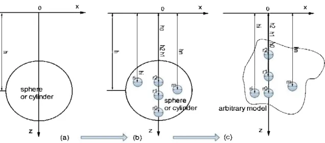
Ensuite, nous généralisons l'eq.5 en divisant le modèle de la sphère en un nombre infini de petites sphères. Leur centre de profondeur d'enfouissement et leurs rayons sont ho, h1, h2, ... hi, ... , hn et r0, r1, r2, ... ri, ... rn, respectivement (figures 2.6b et 2.6c). Basées sur le principe de superposition, les anomalies magnétiques de différents corps aux différentes profondeurs peuvent être considérées comme différents signaux de fréquence; et la réponse du nombre infini de petites sphères est :
n
za(x)
=
L
zi(x) (6)l ~O
Son spectre de transformée de Fourier est également la somme des spectres de la transformée de Fourier de Z1 (x) :
n
Za(kx)= L:Z,(kx) (7)
J~O
Où Z, (kx ) est le spectre de transformée Fourier de zi (x) .
Selon l'éq.l et l'éq.7, nous pouvons obtenir une formule liant le centre de la profondeur d' enfouissement et le nombre d'onde maximale pour une petite sphère arbitraire ou un cylindre horizontal arbitraire. Et si nous considérons ri comme infiniment petit, lorsque n~o, les petites sphères deviennent des points, nous pouvons donc simplifier l'éq.6 comme suit :
(8)
Dans la nature, une véritable source d'anomalie comme une sphère n'existe pas. Les anomalies magnétiques sont principalement générées par des corps irréguliers comme le montre la figure 2.6c dans le Chapitre II de ce mémoire. Nous supposons qu' il existe une anomalie magnétique en un point arbitraire dans l 'espace, et que c'est un certain nombre de petites sphères qui génère cette anomalie. Vu que le spectre de puissance Zi(kxi) obtenu à partir de la réponse magnétique de chaque sphère a une valeur maximale de puissance, et que sa profondeur d'enfouissement h et le nombre d'ondes maximales kxmax sont liées par l ' éq.5, par conséquent, nous pouvons déterminer la profondeur d'enfouissement de chaque sphère par l'analyse de leur spectre de puissance à des positions arbitraires spatiales. Ultimement, nous pouvons déterminer
Xll
une distribution de la source des anomalies magnétiques. Nous appelons cette dernière Imagerie de profondeur.
Nous avons généré les anomalies de 14 petites sphères et ensuite utilisé l'eq.8 pour estimer leur profondeur d'enfouissement. Les résultats sont présentés au tableau 2.2 dans le Chapitre II de ce mémoire. L 'erreur relative moyenne de l'estimation des sources profondes et peu profondes est de 21 %. Cependant 1 'erreur relative est de seulement 5 % pour les sources qui se trouvent à une profondeur supérieure à 150 mètres. Il semble que plus la profondeur d'enfouissement de la source augmente, plus l ' erreur d' estimation diminue (figure 2.7). La méthode d' imagerie de profondeur sera donc utile pour localiser des corps enfouis profondément.
2.2 Analyse du spectre de puissance pour les modèles complexes
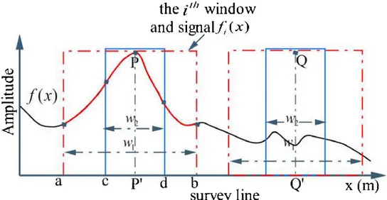
Les amplitudes du spectre de puissance représentent les intensités de susceptibilité ou de magnétisation à des fréquences différentes pour chaque station. Le long d'une ligne d'observation du champ magnétique, nous avons une série de données
fz
(x) qui se trouvent dans la ie fenêtre comme le m ontre la figure 2.8 dans le Chapitre II. En utilisant la m éthode de transformée de Fourier rapide (FFT), nous obt enons un ensemble de donnéesF;
(kx) qui est considéré comme la distribution des amplitudes correspondant à des fréquences différentes à une st ation (P ). Cette m ême procédure est répète N fois pour chaque station. N ous avons résumé cette procédure de calcul de façon schématique à la section 2.5 dans le Chapitre IL La série de données {F; (kx)} est dans le dom aine espace-nombre d'ondes. Les méthodes STFT (Short-time Fourier Transform; Jont B . Allen, 1977), W T (Wavelet Transform; Morlet, 1982; Chui, Charles K., 1992) et ST (S Transform; Stockwell R. G., Mansinha L. , Lowe R. P., 1996 ; Stockwell, 1999) peuvent être utilisées pour transformer les données spatiales dans le dom aine de fréquence :f( ) x -~--~ Transfo rm tools F( k ) x ,
x (9)
En intégrant l' eq.8 dans l 'eq.9, nous obtenons les données d 'imagerie dans le domaine spatial :
F(x,h)
(10) Où:
x est la ligne d'observation;
h représente la profondeur d'enfouissement du corps causatif de l'anomalie;
kx représente la longueur d'onde ;
f(x) représente la réponse du champ magnétique (courbe noire);
fi(x) représente les données interceptées par laie fenêtre (segment de la courbe rouge).
X111
Nous considérons que l'amplitude (spectre de puissance) est un attribut pertinent de l'anomalie magnétique pour chaque longueur d'onde (ou chaque profondeur) à une station. Donc, cet attribut inclut des informations de l'intensité de la magnétisation et de la profondeur du corps magnétique.
Nous avons appliqué la nouvelle méthode aux six modèles de sphère. Pour chaque modèle, l'azimut de la ligne d'observation est rrl2. Les sphères sont dans un champ magnétique aimanté verticalement. Elles ont le même niveau de magnétisation et la susceptibilité est de 0.2 SI pour chaque sphère. La force du champ magnétique incité est de 50 000 nT. Différents paramètres géométriques sont présentés par les figure s 2.32-2.37 dans le Chapitre II du mémoire.
Modèle 1 : Telles que présentées à la figure 2.32, deux sources d'anomalies sont très bien
définies par leur spectre de puissance, et leur position dans l'espace estimé par l'imagerie de profondeur est identique à celle du modèle. La profondeur du centre de la sphère correspond à la profondeur de la partie supérieure du spectre de puissance (partie inférieure de la figure 2.32).
Modèle 2 : Nous ajoutons une sphère plus profonde en dessous d'une des deux sphères du
modèle 1 (panneau supérieur de la figure 2.33), à la position x=O. Ces deux sphères empilées verticalement génèrent une zone rubanée du spectre de puissance élevée (partie inférieure de la figure 2.33). Nous ne pouvons pas distinguer les deux corps facilement, mais nous pouvons deviner qu'il y a deux sources parce que la largeur du spectre de puissance change avec la profondeur et parce que la zone de puissance élevée ne se ferme pas à la profondeur. L'estimation de la position latérale de source peu profonde à l'emplacement de x=250 rn correspond exactement à la position du modèle; c'est aussi le cas pour la position latérale des deux modèles à
XlV
x=O m. Pour la précision sur la profondeur des sphères, celle qui est enfouie à 100 mètres de profondeur est marquée par le début de l'amincissement de spectre.
Modèles 3 et 4 : Ces modèles sont composés d'un cylindre horizontal au-dessus d'une plaque épaisse (modèle 3), ou sous la plaque épaisse (modèle 4); ils s'étendent à l'infini le long de l'axe y. L'inclinaison du champ magnétique est de 300 et l'azimut du profil d'observation est zéro. Les positions du modèle et leurs paramètres géométriques sont présentés à la figure 2.34 dans le Chapitre II. Pour le modèle 3, les emplacements du centre du cylindre sont (0, 0, 50) et (0, 0, -150) respectivement, l'emplacement du centre de la plaque épaisse est (0, 0, -1 00) pour les deux modèles.
Selon la forme du spectre habituel des sphères (centré et fermé), le spectre de puissance du modèle 3 implique qu'il existe une autre source profonde qui a une géométrie différente de sphère ou de cylindre. Nous pouvons voir que le haut du spectre de puissance (figure 2.34) définit très bien la profondeur de la sphère. En plus, il y a une discontinuité de spectre qui correspond à la profondeur du centre de la plaque épaisse, ce qui est cohérent avec les modèles 1 et 2. Nous avons distingué ces deux corps superposés verticalement avec succès puisque la plaque épaisse a un grand volume par rapport à la sphère. Si cette plaque épaisse se positionne au-dessus d'un cylindre ou d'une sphère qui est caché plus profond (figure 2.35), elle pourrait engendrer une fausse interprétation et laisser croire que la zone d' anomalie du spectre de puissance représente un seul corps allongé verticalement (figure 2.35). Toutefois, la zone d'anomalie du spectre est estimée entre 100 et 200 mètres de profondeur. Celle-ci récupère les deux corps et représente toujours une interprétation raisonnable.
Modèle 5 : Comme nous ne sommes pas en mesure de distinguer le cylindre profond à partir du prisme dans le modèle 4, nous mettons le cylindre en lieu profond (200 mètres), et nous augmentons son rayon à 50 mètres afin d'obtenir sa réponse (figure 2.36a). L'inclinaison du champ magnétique est de 30 degrés.
À la figure 2.36b-c, nous pouvons clairement distinguer deux zones irrégulières du spectre de puissance. C'est définitivement prouvé que la méthode d'imagerie de profondeur peut séparer les sources superposées verticales si elles sont à part à une certaine distance.
xv
Mais la position du centre de la source dévie de 1 'emplacement (x=O); nous nous demandons si elle peut être causée par l'inclinaison magnétique. Ainsi, nous avons modifié l'inclinaison à 90 degrés (aimantation verticale) comme dans le modèle 6 suivant.
Modèle 6 : Pour le modèle 6, tous les paramètres géométriques et physiques sont les mêmes que pour le modèle 5, à l'exception de l'inclinaison du champ magnétique est de 90 degrés.
Nous avons toujours les mêmes conclusions avec le modèle 5. Le modèle 6 a montré que la déviation de position n'est pas provoquée par l'inclinaison.
2.3 Analyse du bruit
Nous avons analysé l'impact du bruit sur la méthode d'imagerie de profondeur en utilisant le bruit aléatoire et le bruit blanc Gaussien. Le bruit peut provoquer une déformation grossière au résultat de la transformée de Fourier. Comme le NSR augmente, les composants de DC deviennent ainsi plus évidents.
Une discontinuité se produit lors de l'utilisation de la transformation de Fourier, il s'appelle le phénomène de Gibbs (effet du bord). Souvent, nous devons choisir une fenêtre pour lisser les points discontinus. Afin d'obtenir des fonctions appropriées de la fenêtre, nous avons étudié une série de fonctions et leur impact sur le signal, y compris la fenêtre gaussienne, la fenêtre de Blackman, la fenêtre Hamming, la fenêtre de Hanning et la fenêtre de Bartlett. Pour un même nombre d'échantillonnages, le spectre de signal lissé par la fenêtre gaussienne, la fenêtre de Hamming et la fenêtre de Bartlett est meilleur que par la fenêtre de Hanning et de Blackman. Pour une même fenêtre, un grand nombre d'échantillonnages correspond à un spectre plus lisse; cependant le nombre d'échantillonnage n'est pas assez grand pour affecter la vitesse de calcul.
2.4 Problème de source équivalente
Afin d'analyser le problème d'équivalence de la source (plusieurs sources peuvent produire une anomalie similaire), nous avons fait une série de modélisations utilisant des modèles de prismes, de sphères, de corps polygonaux 2D.
Le principe d'équivalence de sources a été utilisé pour des transformations du champ potentiel, par exemple, pour les dérivations directionnelles, continuation vers le haut ou vers le
XVl
bas. Nous avons discuté de ce problème en citant deux types de sources d'équivalence : source des points confinés à une surface et des corps ayant une géométrie différente ou se situant à différente profondeur. Selon les résultats de modélisations, nous concluons que : 1) le premier type d'équivalence de source ne contient aucune information de la géologie; 2) plusieurs corps ayant une géométrie différente peuvent générer une anomalie magnétique vraisemblable, mais ils doivent se situer à la même profondeur. Cette équivalence ne pose pas de problème dans l'interprétation des données magnétiques ou gravimétriques, car la résolution spatiale de l'interprétation consiste à la localisation réelle de sources. En tentant de simuler certains corps équivalents qui sont plus profonds que le corps causal, nous avons démontré que ce type de source équivalente n'existe pas en réalité.
XVll
3
ÉTUDE DE CAS
Nous avons appliqué la méthode d'imagerie de profondeur aux données réelles recueillies à la mine Galien, dans la ceinture de roches vertes de l'Abitibi, au Québec.
3.1 Contexte géologique
Le dépôt de la mine Galien des sulfures massifs volcanogènes et des roches volcaniques forme une inclusion dans la granodiorite du lac Dufault (figures 3.1 et 3.2). Les contacts de la granodiorite du Lac Dufault avec les roches encaissantes sont partiellement connus. Le contact nord s'incline vers le sud et il recoupe gisement Galien. La lentille principale de la minéralisation recouvre une séquence volcanique falisque nommée Formation rhyolitique Sud du lac Dufault, dont la composition varie de tacite à andésite.
Du stockwerk à pyrite est présent dans les roches du plancher du dépôt; ici, l'altération est caractérisée par la séricitisation et la silicification. La déformation progressive est plus intense dans cette zone, celle-ci est marquée par une schistosité pénétration parallèle au contact inférieur de la lentille minéralisée. Les sulfures massifs sont hébergés dans ce qu'on appelle un «horizon de tuf contenant des phénocristaux de quartz» (Riopel, 2001).
La lentille principale de la mine Galien a environ 250 mètres de longueur et 80 mètres de largeur, avec une petite lentille profonde située au sud-ouest à plus de 200 mètres de profondeur (figure 3.2). La lentille principale se compose principalement de pyrite, mais contient jusqu'à 20% de sphalérite (Guimont et Riopel, 1998). Les deux lentilles sont associées à une vaste minéralisation disséminée dans la Formation rhyolitique sud du lac Dufault.
3.2 Description des données magnétiques
Les données magnétiques utilisées dans cette étude proviennent principalement d'un levé aéroporté de MEGATEM en 2003 (Fugro airbome surveys). Le Scintrex CS-2 monté sur un avion Tash-12 mesure l'intensité totale du champ magnétique de la terre à une altitude de 70 mètres au-dessus du sol. Les données magnétiques sont ensuite traitées à 1 'aide du logiciel Geosoft. Un champ linéaire est également supprimé en utilisant Geosoft pour éliminer l'effet régional; les anomalies résiduelles sont réduites au pôle.
xvm
La réponse magnétique du dépôt de la mine Galien sur la carte des anomalies résiduelles est relativement petite, environ de 300 à 700 nT. Mais au sud du dépôt de la mine Galien, les valeurs de la réponse magnétique sont élevées ce qui attiennent un maximum de 2800 nT dans le sud-ouest de la zone d'étude (figure 3.4 dans le Chapitre III).
3.3
Résultats et interprétations
À la figure 3.1, nous pouvons observer que le dépôt de la mine Galien est dans un contexte géologique complexe. Nous avons appliqué la méthode d'imagerie de profondeur pour recouvrir une distribution de la susceptibilité magnétique en profondeur à l'intérieur d'une petite zone autour du dépôt de la mine Galien. Un modèle géologique 3D a été construit par l'interprétation des données de trous de forage pour cette zone (figure 3.5). Nous voyons à la figure 3.2 que les intrusions felsiques porphyriques ont perturbé la séquence de rhyolite, ce qui implique que la géologie réelle du dépôt de la mine Galien serait beaucoup plus complexe que le modèle géologique 3D montré.
Nous avons procédé au calcul d'imagerie de profondeur le long de dix profils orientés 0-E et de neuf profils orientés S-N (la localisation de ces lignes est indiquée à la figure 3.4). En comparant les résultats d'imagerie de profondeur avec la géologie comme de la surface (figure 3.7), il semble que l'amplitude du spectre de puissance de la Formation rhyolitique est inférieure à celui des intrusions felsiques porphyriques (à la gauche de la figure 3.7). Selon l'image du spectre de puissance, les intrusions felsiques porphyriques s'étendent vers l'est.
Le contact nord entre la rhyolite et la granodiorite est clairement démontré par la discontinuité du spectre de puissance (figures 3. 7 et 3. 8). Il est possible que le contact nord soit incliné vers le sud au niveau peu profond, mais on ne peut pas ignorer l'existence d'une source profonde qui se situe dans le sud-ouest de la zone d'étude. Cette source s'étendait vers le nord-est en profondeur (figure 3. 7). Son spectre de puissance a une amplitude élevée de 80000 à 100000 nT. Il pourrait être la source des intrusions felsiques porphyriques. La figure 3.7 nous montre une fois de plus la discontinuité du spectre de puissance dans le nord (à gauche) et la direction du pendage de contact nord vers le SW à faible profondeur (à droite).
Nos résultats d'interprétation par la méthode d'imagerie de profondeur ont montré que la structure souterraine dans la zone de la mine Galien est très hétérogène, ce qui est conforme à la
Xl X
carte géologique détaillée (figure 3.2). Notre étude a proposé une nouvelle approche pour l'interprétation des données magnétiques.
xx
4
CONCLUSIONS
Nous avons étudié les caractéristiques du spectre de puissance du champ magnétique dans le domaine de fréquence, ce qui nous a permis de constater qu 'il y a une corrélation entre la puissance de spectre et la profondeur d'enfouissement de la source de l'anomalie. Nous avons développé une nouvelle formule mathématique pour exprimer la relation entre la profondeur d'enfouissement et le nombre d'ondes du spectre de puissance. Nous avons ensuite généralisé cette formule à une situation générale et développé une nouvelle méthode d'imagerie en profondeur pour l'interprétation des données magnétiques.
En utilisant des modèles synthétiques, nous avons testé cette nouvelle méthode. Pour les sources horizontales, nous pouvons estimer leur profondeur et leur localisation latérale à haute précision. Lorsque la profondeur d'enfouissement des sources augmente, nous obtenons une plus grande précision de l'estimation par l'analyse de leur spectre de puissance. Pour les corps superposés verticalement, nous pouvons estimer précisément la profondeur de la source peu profonde. Si un petit corps recouvre un corps plus grand, nous pouvons facilement les séparer par une discontinuité du spectre. Toutefois, lorsque le corps plus grand cache un petit en dessous, nous ne pouvons les distinguer que s'ils sont suffisamment espacés.
Pour les anomalies magnétiques, le bruit peut provoquer une déformation grossière au résultat de la transformée de Fourier comme le NSR augmente ; ainsi les composants de DC deviennent plus évidents. L'effet du bruit sur les composants avec un petit nombre d'ondes est plus petit que ceux avec un grand nombre d'ondes pour le même rapport de signal-bruit.
À propos du problème d'équivalence de la source, selon nos études, il est possible que plusieurs corps magnétiques à la même profondeur puissent produire une seule anomalie. Cependant, il n ' affecte que la forme du corps causal sans affecter le positionnement précis de la source, ce qui est le plus important facteur dans l' exploration minière. Pour un empilage vertical de plusieurs corps magnétiques, l'effet d'augmentation de la profondeur d'enfouissement sur la forme d'anomalie est non compensable par la variation de la susceptibilité. Par conséquent, il est donc possible de distinguer les corps à différentes profondeurs par notre nouvelle méthode.
L' effet du bord dans la transformation de Fourier (le phénomène de Gibbs) est considéré dans notre calcul. En utilisant des fenêtres pour lisser le signal, les résultats de la transformée de
X Xl
Fourier sont bien meilleurs que ceux du signal d'origine. Le principe de choisir une fenêtre est qu'un nombre suffisant de points d'échantillonnage, en ajustant les paramètres de la fonction de fenêtre, fait le signal original lisse de zéros.
À travers l'étude de cas de la mine Galien, nous démontrons également que la méthode d'imagerie de profondeur peut produire un modèle complexe sans aucune contrainte de discrétisation du modèle. Nous allons continuer à travailler vers des situations géologiques plus complexes. L'ajout d'informations connues, comme la contrainte dans la procédure de calcul, permettra d'améliorer la résolution spatiale. Nous continuerons également à trouver le lien intrinsèque entre le spectre de puissance et les propriétés physiques, comme la susceptibilité magnétique.
XXll
TABLE OF CONTENTS
ACKNOWLEDGEMENTS ... ... ... ... ... III RÉSUMÉ ... ... ... ... ... ... IV ABSTRACT ... VI CONDENSÉ EN FRANÇAIS ... VII TABLE OF CONTENTS ... XXII LIST OF TABLES ... XXIV LIST OF FIGURES ... XXV LIST OF SYMBOLS AND ABBREVIATIONS ... XXIX CHAPTER 1 INTRODUCTION ... ... ... ... ... 1
1.1 Magnetic field ... ... ... ... ... 1 1.2 Methodological development and research hypotheses ... 2 1.3 Objectives ... ... ... ... ... ... 5
CHAPTER2 THE DEVELOPMENT OF DEPTH IMAGING METHOD BASED ON
SPECTRUM ANALYS IS ... ... ... ... ... 6 2.1 Magnetic anomal y of a sphere mo del ... 6 2.2 Power spectrum analysis of single or multiple spheres ... ... ... 7 2. 3 Magnetic anomal y of a thick prism mo del.. ... ... ... 11
2.4 The relationship between wave-number and depth ... ... ... 13 2. 5 Power spectrum analysis for complex models ... 18 2. 6 Analysis of noise and t he Gibbs phenom enon ... ... ... 21 2. 6.1 Noise analysis ... 21 2. 6.2 Gibbs phenomenon and the choice ofsmooth w indow ... 3 1 2.7 Modeling t est ... 36
XX111
2.8 Problem of equivalent source ... 47 2.8.1 Equivalent surface or layer. ... ... ... ... 47 2. 8. 2 Equivalent bodies ... 48 CHAPTER3 CASE STUDY ... 54 3.1 Geology of the Galien Volcanogenic Massive Sulfide Deposit ... 54 3.2 Magnetic data description ... 56 3.3 Data processing results and interpretation ... 58 CONCLUSION ... 64 REFERENCES ... ... ... ... ... ... 66
XXlV
LIST OF TABLES
Table 2.1: Parameters of three sets of sphere mo dels ... ... ... ... 9 Table 2.2: Estimation ofthe depth of 14 spheres ... 17 Table 2.3: List ofparameters oftwo spheres ... 22 Table 2.4: Parameters of prism 1 - 3 ... 50 Table 2.5: Parameters ofprism 6, sphere and 2D polygonal body ... 52 Table 3.1: Magnetic susceptibilites of rocks and minerais ... 60 Table 3.2: Koenigs berger rations (Q) for sorne rocks ... 60
xxv
LIST OF FIGURES
Figure 2.1: Geomagnetic field elements ... ... ... ... 6 Figure 2.2: a) two sphere models; b) upper panel, magnetic anomalies of the model 1 calculated from eq. 1 and eq. 2 on the upper panel c) and those ofthe model2 on the lowerpane1.. ... 8 Figure 2.3: vertical magnetic anomalies (left) and their Power spectrum (right) of three sets of
models. The results of Power spectrum are normalized by the ir own maxima ... ... 11 Figure 2.4: Elements ofthick prism ... 12 Figure 2. 5: Vertical magnetic anomalies (upward) of thick prisms and the ir Power spectrum at different depths ... 13 Figure 2.6: Discretization from sphere model to an arbitrary model ... ... ... 16 Figure 2.7: Correlation between depth and wave-number ... 18 Figure 2.8: Sketch of space-wavenumber-domain analysis ... ... ... 19 Figure 2.9: Complex models with three (al) and two spheres (a2); STFT spectrum of their
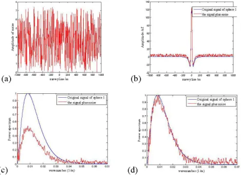
magnetic anomalies (bl and b2) ... ... ... ... ... 21 Figure 2.10: NSR=l%, (a) Random noise (NSR=l %), (b) original signal and the signal plus noise
and ( c) spectrum of FFT of shallow sphere 1 ... 23 Figure 2.11: NSR=3%, (a) Random noise (NSR=3%), (b) original signal and the signal plus noise, (c) spectrum of FFT and (d) spectrum of FFT deleted DC component of shallow sphere 1 ... ... ... ... ... ... 23 Figure 2.12: NSR=5%, (a) Random noise (NSR=5%), (b) original signal and the signal plus noise, (c) spectrum of FFT and (d) spectrum of FFT deleted DC component of shallow sphere 1 ... 24 Figure 2.13: NSR=lO%, (a) Random noise (NSR= lO%), (b) original signal and the signal plus noise, (c) spectrum of FFT and (d) spectrum of FFT deleted DC component of shallow sphere 1 ... 24 Figure 2.14: NSR= l %, (a) Random noise (NSR= l %), (b) original signal and the signal plus noise and ( c) spectrum of FFT of deep sphere 2 ... 25
XXVl
Figure 2.15: NSR=3%, (a) Random noise (NSR=3%), (b) original signal and the signal plus noise, ( c) spectrum of FFT and of deep sphere 2 .... ... ... ... 25 Figure 2.16: NSR=5%, (a) Random noise (NSR=5%), (b) original signal and the signal plus noise, ( c) spectrum of FFT and ( d) spectrum of FFT deleted DC component of deep sphere 2 ... 26 Figure 2.17: NSR= 10%, (a) Random noise (NSR= 10%), (b) original signal and the signal plus noise, ( c) spectrum of FFT and ( d) spectrum of FFT deleted DC component of deep sphere 2 ... 26 Figure 2.18: NSR=1%, (a) WGN (NSR=1%), (b) original signal and the signal plus noise, (c) spectrum of FFT of shallow sphere 1 ... 28 Figure 2.19: NSR=3%, (a) WGN (NSR=3%), (b) original signal and the signal plus noise, (c) spectrum of FFT of shallow sphere 1 ... 28 Figure 2.20: NSR=5%, (a) WGN (NSR=5%), (b) original signal and the signal plus noise, (c) spectrum of FFT of shallow sphere 1 ... ... ... ... 28 Figure 2.21: NSR=8%, (a) WGN (NSR=8%), (b) original signal and the signal plus noise, (c) spectrum of FFT of shallow sphere 1 ... 29 Figure 2.22: NSR= 1%, (a) WGN (NSR= 1%), (b) original signal and the signal plus noise, (c) spectrum of FFT of deep sphere 2 ... ... ... ... 29 Figure 2.23: NSR=3%, (a) WGN (NSR=3%),(b) original signal and the signal plus noise, (c) spectrum of FFT of deep sphere 2 ... ... ... ... 29 Figure 2.24: NSR=5%, (a) WGN (NSR=5%), (b) original signal and the signal plus noise, (c) spectrum of FFT of deep sphere 2 ... ... ... ... 30 Figure 2.25: NSR=8%, (a) WGN (NSR=8%), (b) original signal and the signal plus noise, (c) spectrum of FFT of deep sphere 2 .... ... 30 Figure 2.26: Signal with a constant signal with zero frequency ... 32 Figure 2.27: Analysis for the impact of Gaussian window on signal: w indow functions (left), spectrum ofFouriertransform about original signais and signais smoothed (right) ... 33
XXVll
Figure 2.28: Analysis for the impact of Blackman window on signal: window functions (left), spectrum ofFouriertransform about original signais and signais smoothed (right) ... 33 Figure 2.29: Analysis for the impact of hamming window on signal: window functions (left), spectrum ofFouriertransform about original signais and signais smoothed (right) ... 34 Figure 2.30: Analysis for the impact of hanning window on signal: window functions (left), spectrum ofFouriertransform about original signais and signais smoothed (right) ... 35 Figure 2.31: Analysis for the impact of Bartlett window on signal: window functions (left), spectrum ofFouriertransform about original signais and signais smoothed (right) ... 36 Figure 2.32: Model1 (upper), the depth imaging result (lower) ... 37 Figure 2.33: Model2 (upper) and their depth image (lowers) ... 39 Figure 2.34: Model 3 (upper) and Depth imaging (lower) for the superposition of the cylinder over (left) or under (right) the prism, window width is 256 ... .41 Figure 2.35: Model 4 (upper) and Depth imaging (lower) for the superposition of the cylinder
undem eath the prism , win dow width is 256 ... ... ... ... 43 Figure 2.36 : Model 5 (left) and Depth imaging (right) processed by window function with
different width for the superposition ofthe cylinder and the prism ... 44 Figure 2. 37: Model 6 (as shown in figure 2.37a) and Depth imaging results processed by window functions with different w idth for the superposition ofthe cylinder and the prism ... 46 Figure 2.3 8: A cylinder at the depth of250m and its equivalent-sources at different depth ... 48 Figure 2. 39 : Equivalent source ofprisms which have the same (or different) center depth with the causative anomal y (Prism 1) ... ... ... ... ... 51 Figure 2.40: 2 dimensional (2D) polygonal body ... ... ... ... 53 Figure 2.41: Responses of prism , sphere and 2D polygonal body ... ... ... 53 Figure 3.1: Regional geology map of the Galien area ... 55 Figure 3.2: Det ail geological map around the Galien deposit, overlapped by magnetic survey
lines with flight direction over the Galien deposit (left), the geological cross-section along line A-B ... 56
xxvm
Figure 3.3: Survey system and its configureation ... 57 Figure 3.4: Residual magnetic anomalies over the Galien deposit, the blue cycle indicates Galien ore body location, white lines represent magnetic data interpretation profiles ... 58 Figure 3.5: Top view of 3D model (left), the 3D geological model (right) ... ... 59 Figure 3.6: Comparisons between the depth imaging at the depth of 75 rn (left), detail geological map (middle) and 3D geological model (right) ... ... ... ... 59 Figure 3.7: Two cross-sections from the depth imaging 3D model (right) and their location over the 3D geological model (left) ... 61 Figure 3.8: 3D view of the depth imaging results from two cross-sections ... 62 Figure 3.9: Three cross-sections from the depth imging 2D model (left) and their location on the detail geological map (right) ... 63
LIST OF SYMBOLS AND ABBREVIATIONS
Abbreviation or Symbol A, B, C, D A'a, b
c f(x) F(x, k,J F(x,h) FFT GWN h I M MAX(abs(S)) Definition Api ces of prismMagnetic azimuth of profile Geometrie parameters ofbody Constant
Data in spatial domain
Data in space-wavenumber domain Data in 2-dimensional spatial domain Fast Fourier transform
White Gaussian Noise
Burial depth of geological body Depth to the center of body
Magnetic inclination
Effective magnetization inclination Wave number of x-axis
Wave number of y-axis
Wave number corresponding to the maximum value of Power spectrum
Total intensity of magnetization Effective magnetization
X-axis' component of M Y-axis' component of M Z-axis' component of M
Maximum of the absolute values of signal S ,
n
1 = (Z,m,n) iî2 = Clo,mo,no) NSR nNO
random(O, 1) 2b 2-D, 3-D flo a K r Magnetizing directionDirection ofthe normal geomagnetic field on the Measurement profile
Percent ratio of noise to signal Numeral
Random noise distributed uniformly
White Gaussian noise with the variance of 1 White Gaussian noise with specifie variances Power spectrum
Distance between two points
Random sequence distributed in the interval [0, 1] Signal of magnetic response
Survey line or x-axis
Vertical magnetic anomaly component in spatial domain Vertical magnetic anomaly component in wave number domain
Thickness of prism
Two dimensional, three dimensional Circumference ratio (PI)
Magnetic permeability of free space The dip angle of the prism
Magnetic susceptibility of rocks and minerais Radius of sphere or cylinder
Angles between rA, rB, re , rD and the verticalline The total magnetic anomal y field in spatial domain The total magnetic field anomaly in wave number domain
1
CHAPTERl
INTRODUCTION
1.1 Magnetic field
The Earth magnetic field is generated by internai electric currents (mainly by the Earth's outer core, and the magnetization of rocks in the ernst) but also from ionosphere and magnetosphere. The Earth magnetic field can be very roughly approximated by a dipole magnet (William Gilbert, 1600), which is defined by its angles relative to the north (declination) and relative to the horizontal (inclination), called geomagnetic field.
In the middle of 17th century, Swedes (1640) used magnetic compasses to prospect for magnetite in Zhalkovsky (2008). Thaln made a simple magnetometer in 1879 and the magnetic method was then formally used for mineral exploration. In 1915, Schmidt invented the knife edge-type magnetometer (balance), the magnetic method started to be used extensively in iron prospecting, also for studying the geological structure. In 1936, Rogachev succeeded in inventing the airborne magnetometer, and improved the measurement range and the efficiency of the instrument. After the Second World W ar, the airborne magnetic method was widely used in prospecting metallic deposits over extensive area. In the 20th century, in the 50's and early 60's, the proton-precession magnetometer was used for marine prospecting. At the same time, the magnetic method be gan to be used for the study oftectonic structures and geological mapping.
Since the strength of the magnetic field from rocks (high iron content) is small compared to the strength of the main magnetic field of the Earth, the Spherical harmonie analysis method (Gauss, 1838) was used to simulate Earth's main magnetic field in order to extract struct ural geology information of the ernst. In 1968, the International Association of Geomagnetism and Aeronomy (IAGA) first proposed the 1965.0 Gaussian spherical harmonie analysis models. This model was approved in 1970 by IAGA and called the international geomagnetic reference field model (IGRF). This model, which is regarded as the mathematical model of the main geomagnetic field and its secular variations, consists of a set of Gaussian spherical harmonie coefficients and annual gradient coefficients. Alldredge recreated the rectangular harmonie analysis (RHA) in 1981, and applied RHA to surface data (1981, 1982, and 1983). Nakagawa and Yukutake (1985) and Nakagawa et al. (1985) extended its application to the analysis of satellite data. The RHA used a plan to approximate spherical surface; therefore the area of the model is
2
limited. In order to overcome this problem, and to use the rectangular coordinate system to replace the spherical coordinate system, Haines (1985) designed the spherical cap harmonie analysis (SCHA) to simulate the IGRF. Since then, the SCHA is used to provide a magnetic reference field of Canada. Because of the secular variation of the geomagnetic field, spherical harmonie coefficients are republished every five years, and the geomagnetic map is redrawn. Recently, the National Geophysical Data Center (NGDC) and the British Geological Survey developed the 2010.0 - 2015.0 World Magnetic Model (WMM). By using those models, after subtracting the main magnetic field and correcting extemal sources, geophysicists use the residual magnetic field for mineral exploration and for studying underground structures.
Magnetic exploration has many merits: the magnetometer is light and easy to handle, has high work efficiency and low cost. The most important is that the airbome magnetic method can measure extensive areas in a short period of time; and the measurement is not restricted by the terrain relief, providing global magnetic field anomaly information. This method is therefore extensively used in mineral and oil prospecting, hydrogeology, environmental sounding and for monitoring ofthe movement oftectonic plates.
1.2 Methodological development and research hypotheses
The availability of magnetic data increases with time, mainly due to those collected from airbome surveys. However, we still have limited access to efficient interpretation tools for magnetic data. There is no clear relationship between the magnetic signal (anomaly) and the rock types as well as the depth of the magnetic anomaly's source, due to large variability of geology in nature. Barton (1929), Nabighian (1962), Bhattacharya (1964), Nagy (1966), and Hjelt (1972, 1974) simulated magnetic anomalies with simple geometries such as a sphere, a cylinder and a plate. Talwani and Ewing (1960), and Talwani (1965) proposed the numerical integration method to simulate arbitrarily shaped bodies . These numerical methods may be cumbersome to use, yet the body to be mode led has to be divided into a large number of thin horizontal laminas (Bamett, 1976). Parker (1973), Dorman and Lewis (1974) presented other numerical methods which are well used in potential fields ; these methods involve a series expansion in terms of the Fourier transforms of powers being considered (Bamett). Paul (1974) developed a solution for potential fields based on a homogenous polyhedron composed of triangular facets. Plouff (1976) used polygonal prisms to model the potential field. Bamett (1976) developed an analytical method for
3
modeling the potential field of a homogenous, arbitrary shaped, three-dimensional body. Okabe (1979) first proposed the 3-D vertex point method to compute the response of a potential field; the main idea is to use polyhedral bodies composed of a set of triangles, which yields high accuracy model. Mareschal (1985), Myoung An, et al. (1990) proposed the solution of potential fields in the frequency domain in order to reduce the computation time. Other methods used in simulating complex models in the spatial domain are developed, as finite element methods (Zeng Hua Lin, 1985; Guan, Zhining, 2005; Wenxiao Zhu, Wansheng Tu, Tian you Liu, 1989) and boundary element methods (Sigh B., 2001; Zheshi Xu, Yunju Lou, 1986). Within the finite element method, there are three approaches: the point element method, the linear element method and the panel method. The point element method can be used in modeling the anomalies whose physical properties are inhomogeneous in horizontal and vertical directions. The linear element method requires that the physical properties are change regularly along straight line. The panel method requires that the physical properties change regularly on a surface.
The magnetic inversion methods have also made a significant progress by recovering an underground susceptibility distribution from magnetic observations. In the 70s, the Hilbert transformation inversion method was used in magnetic interpretation for the estimation of 2-dimensional bodies (Moon, Ushah, 1988; Norden E. Huang, Zhaohua Wu. 2008). In the 80s, a three-dimensional derivative computation was developed (Nabighian, 1984). Werner (1955) proposed a deconvolution method, in which model is composed of a vertical or a dipping plate infinitely extending downward. By solving a set of linear equations, we can estimate the horizontal position, the depth to top, magnetic susceptibility and the magnetized direction of the model. Hartman (1971) used this method in aeromagnetic interpretation, and Hansen (1993) extended it to an interpretation of multiple 2-dimensional anomalies. The Compudepth inversion method, which is based on the Fourier transform, the linear phase filtering and frequency shifting, is used to interpret the position and depth of 2-dimensional bodies (O'Brien, 1972). Wang and Hansen (1990) used it in the interpretation of 3-dimensional polyhedrons. Thompson (1982) proposed the Euler deconvolution which can automatically evaluate the position of the source and rapidly make depth estimates from large amounts of magnetic data. The theory is based upon Euler's homogeneity relationship. Reid et al. (1990) and Mushayandebvu et al.
(2000, 2001) developed this method and resolved the stability problem. U gal de and Morris (201 0) used the cluster analysis technique and resolved the problem of strike and dip angle for
2-4
and 3-dimensional bodies. The source parameter imaging (SPI™) has been presented and developed by Thurston and Smith (1997) and by Thurston, Smith and Guillon (2002); this method assumes either a 2-D sloping contact or a 2-D dipping thin-sheet model and is based on the complex analytic signais.
Stochastic methods have been also widely used in the inverse calculation. In the 60s, Backus and Gilbert proposed the Backus-Gilbert inversion method based on finding the smoothest solution. Tarantola A. (1987) developed a set of theories and methods of probability tomography based on optimization theories, such as the Gauss-Newton method (Chen, Kemna, Hubbard, 2008), the non-linear conjugate gradient method (Kelbert, Egbert, Schultz, 2008) and the Monte Carlo method (Bosch, Meza, Jimenez, Honing, 2006), resolving the divergence problem and the stability problem. After the 90s, the simulated annealing (Rothman, 1986), neural network (Zhining Guan, Junsheng Hou, Linping Huang et al. 1998; Ziqiang Zhu, Guoxiang Huang, 1994) and the genetic algorithm (Berg, 1990; Smith, Scales, Fischer, 1992; Curtis, Snieder, 1997) were presented with improved stability of the solution and speed of convergence. Peter G. Lelièvre and Oldenburg (2006) studied the magnetic forward modeling and the inversion of self-demagnetization effects, then designed a methodology for inverting magnetic data for subsurface magnetization and proposed a 3D magnetic inversion with a complicated remanence. Now, Cokriging, a stochastic inversion, which is applied to provide quantitative descriptions of natural variables distributed in space or in time and space and minimizes the theoretical estimation error variance by using auto- and cross-correlations of several variables (Pejman Shamsipour, et al. 2011 and 2012).
Due to the complexity of the magnetic field caused by one or more geological bodies with inhomogeneous magnetic susceptibilities and of irregular shapes, therefore several assumptions have been made in the above developments, such as a) the shape of the model is regular or simple; b) magnetization is homogeneous within the body and susceptibility is isotropie in the causative body; and c) the remanent magnetization was not considered for most of calculations.
Although simple geological bodies are easy to simulate, complex geological conditions in actual surveys broaden huge the gap between theoretical models and actual geology. Furthermore, by using conventional interpretation tools, different bodies can be easily distinguished from magnetic anomalies if they are horizontally well apart, but hardly
5
distinguishable if they are superimposed vertically. In our study, we proposed a new method in spectrum domain, which identifies not only horizontally distributed sources, but also those superimposed vertically.
1.3 Objectives
One of the challenges in potential field (magnetic and gravity) data interpretation is to determine the depth of different vertical superimposed sources. Bo Holm Jacobsen (1987) applied a filter for mapping the geology at different depth levels; many authors used the upward and downward continuation of potential fields to enhance the signal of shallow or deep sources (Jacobsen, 1987; Trompat, Boschetti, and Homby, 2003; Cooper, 2004; Chen Long-wei, Zhang Hui, and Zheng Zhi-qiang, 2007). However, until now there is no effective method to distinguish them.
The objective of our study is to develop a new interpretation tool in order to separate deep and shallow sources and also try to discriminate magnetic anomalies with different volumes (size of geological body) and magnetic susceptibilities (nature of the anomal y causative body).
CHAPTER2
6
THE DEVELOPMENT OF DEPTH IMAGING METHOD
BASED ON SPECTRUMANALYSIS
We stati from severa! simple physical models and their magnetic field analytic expressions, and then transform them into frequency domain in order to study the relation between the Power spectrum & the wave-number of spectrum and the depth ofvarious models.
2.1 Magnetic anomaly of a sphere model
On Figure 2.1, M indicates the geomagnetic field vector or induced geomagnetic vector, its units is in nT (nanotesla); MH represents its hotizontal component which can be projected onto the X-axis
(Mx)
and the Y -axis(My)
andMz
is its vertical component.x geomagnetic _ _ _ _ _ _ ~orth M H y M5/ - - - . - - - - 'M / ' 1 / / 1 / Mz - - - _/ z
Figure 2.1: Geomagnetic field elements
If there is a ferromagnetic sphere inside of this geomagnetic field, assuming that its remanent magnetization is negligible, it will be strongly magnetized along the geomagnetic field direction, thus, a magnetic anomaly is produced. From a magnetic sUivey on land, the main pru·ameters measured ru·e total magnetic field anomaly (ilT), vettical magnetic anomaly (Za) component can be got by calculating from the total magnetic field anomaly or measurement; by an airbome survey we measure the total magnetic field anomal y (ilT). Their units are in nT.
Outside of the magnetic sphere, the vettical magnetic component Za and the total field anomaly ilT at an ru·bitrary point in space can be expressed by the following equations (Zhining Guan, 2005):
7
Jlom z z hz .
2a = 2 2 2 5 / 2 [(2x - y - ) sm/
4n"(x+y+h) (1)
- 3hx cos 1 cos
A'
+
3hy cos 1 sin A']flom 2 2 2 · 2
fo..T= 2 2 25 /2[(2h-x-y)smJ
4n"(x +y +h )
+(2x2 - y2
- h2) cos2 J cos2 A'+ (2y2 - x2- h2) cos2 J sin2 A' (2) -3xhsin2JcosA' +3xycos2
Jsin2A' -3yhsin2JsinA']
K 47T 3
m = - M - r
flo 3
Where llo is the magnetic permeability of free space; K is the magnetic susceptibility of the
sphere; rn is the magnetic moment of the sphere; r is the radius of the sphere; h is its depth; I is the magnetic inclination; A' is the magnetic azimuth ofthe profile (observations); (x, y, z) are the coordinates of the survey station, z is zero on the surface and the sphere is located at (0, 0, h).
2.2 Power spectrum analysis of single or multiple spheres
The Fourier transform of a vertical magnetic anomal y is written as following:(3)
Where Za (k,J is the Fourier transform of za (x), kx and x are the wave-number and distance respectively; and the wave-number has unit of inverse distance.
In order to easily study and compare results, all of Fourier transform results are normalized. The way to normalize Fourier transform results is that: (1) First we find out the maximum of the magnetic response in frequency domain, (2) then we divide the magnetic response in frequency domain by the maximum, (3) the anomalies in frequency domain are normalized in this chapter ( only in this chapter, but except the section 2. 7 of Chapter II).
W e show two spheres on Figure 2.2a. Assuming that they have the same magnetic inclination (n/2), magnetic azimuth of the profile (n/2), and the magnetic susceptibility ( K) is
0.2SI, the magnetization (T) is 50000nT. The radius of the sphere 1 is 20m and its center is situated at a depth of 30m. The sphere 2 is buried at a depth of 1 OOm; radius of sphere is 35m.
8
In Figure 2.2b, from left to right, they are the response of total magnetic anomal y field of the sphere 1 (fj.T) and its vertical magnetic anomaly component (ZJ along the x-axis crossed the projection of the center of sphere (y=O, x=O), its total magnetic anomaly field and its vertical magnetic anomaly component on the surface of x-y. In Figure 2.2c, they are magnetic response of sphere 2, which are same with that of sphere 1.
2000 f--E
..
tOOO]
o. 0 E ~ x lm ..., 1 0 3 1 sphere 12
.1_() radius: 20m ::::~ V sus: 0.2 sphere 2: radius:'35m, Sus: 0.2zl
'
(b) Za and t.T /nT"
~
T'"
}\\.
~ \../ - tOOO -200 -100 0 tOO 200 Survey tine (x) lm Za and àT /nT 300.---~~~====T=I ~200 ~ .~ tOO o. ~ 0··---~ -tOO -200 -100 0 too 200 SUJvey tine (x} / rn 200 tOO ..ê 0 >. - tOO -200 200 tOO -ê 0 >. - tOO -200 0 200 400 600 800 Za /nT (c) 200 tOO -ê 0 >. - too -2000 500 tOOO tSOO t.T loT
-200 -100 0 tOO 200 x l m -200 -tOO 0 tOO 200x/m
-200 -100 0 tOO 200 x /m 200 tOO -ê 0 >. -tOO -200 0 tOO 200 t.T /nT -200 -100 0 100 200 x / rn
Figure 2.2: a) two sphere models; b) upper panel, magnetic anomalies of the modell calculated from eq. 1 and eq. 2 on the upper panel c) and th ose of the model 2 on the lower panel
9
From Figure 2.2b and 2.2c, we see that as the depth increases, the magnetic anomaly becomes flatter and weaker.
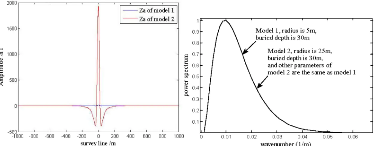
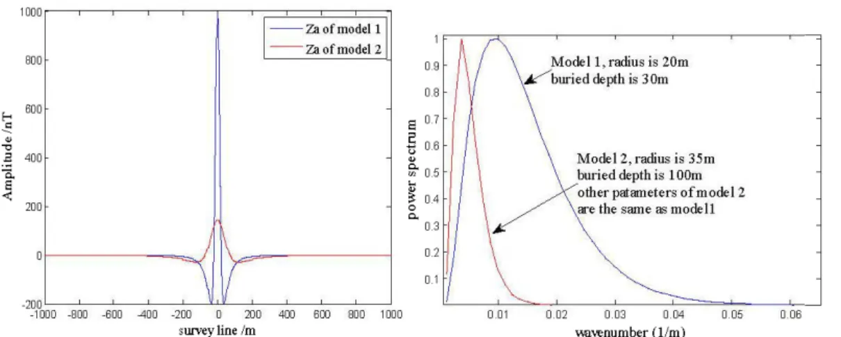
We designed then three sets of models (Table 2.1). The Set 1 consists of two spheres at same location but having different size. The Set 2 is composed of two spheres of same size, but they have different depths. The Set 3 has two spheres of different size, and the small sphere is over the big one. We calculated the magnetic anomaly ofthree sets ofmodels, and then we did the Fourier transform of the vertical magnetic anomaly. Figure 2.3 (a) to (c) show clearly that the magnetic anomaly changes only the amplitude in the space (left figure), however the different depths correspond to different wavenumber in the frequency domain. As the depth of the sphere increases, the wave number becomes smaller. We wonder if we could quantify this feature by the anomaly's attribute related to the depth. Please note that the results of Power spectrum are normalized by their own maxima.
Table 2.1: Parameters of three sets of sphere mo dels
Set 1 (figure 2.3a) Set 2 (figure 2.3b) Set 3 (figure 2.3c) Mode
parameters Modell Model2 Modell Model2 Modell Model2
Radius (r) Sm 25m 20m 20m 20m 35m
Center depth (h) 30m 30m 30m lOOm 30m 100m
Magnetization 50000nT (M) Susceptibility 0.2SI (K) Inclination (I) n /2 Azimuth (A') n /2
2000 1500 E-< ..::; 1000 "'
.,
~ ë.. ~ 500\
v
-500 -1000 -800 -600 -400 -200 200 survey line lm ~ --Za of model1 - - Za of mo del 2 0 .9 0 .8 s 0 7 ~ 0 .6 " ~ 0 .5 Il ::: 04 0""
0 .3 02 0 .1 400 600 800 1000 0 .01 Mode! 1 , radius is 5m, buried depth is 30m Model2, radius i s 25m, buried depth is 3 Om, and other parameters of mode! 2 are the same as mode! 10.02 0 .03 0 .04 0 .05 0 .00
wavenumber (1/m)
10
Figure 2.3a: vertical magnetic anomalies (left) and their Power spectrum (right) of the first set of models E-< --e "' "'0 ~ c.. ~ 100 0 ' El) 0 60 0 40 0 20 0 0
\
-20 0 -1000 -800 -600 -400 -200 ~ -- Zaofmodel1 - -z. ofmodel21
(
0 .9 08 0 .7 E ~ 0 6 ~0 5 ~ 0 .4 ~ c.. 0 3 0 .2 01 200 400 600 800 1000 '"""Y line /rn 0 0 01Modell , radius is ZOrn ,
buried depth is 3 Om
/
Model2 , radius is 20m,burieddepth is 100m , and other parameters of mo del 2
are the s am e as mo del 1
002 0 03 004 00 5 0 0 6
w.tvenumber (1/m)
Figure 2.3b vertical magnetic anomalies (left) and their Power spectrum (right) of the second set ofmodels
1000 000 ~ - Zaofmodell - Za of mode! 2 f-< 600 -!' ~ ., 2 400 ~ s -<: 200
l
1(
-200 -1 000 -800 -600 -400 -200 0 200 400 600 000 1000 survey line /rn s 0.7 ~ 0 6 " ~ 0.5 ... ~ 0.4 0""
0.3 0 2 0 1Mode Il, radius is 20m
~buried depth is 3 Om
Moclel2, radius is 35m buried depth is 1 QOm other patameters ofmodel2 are the same as mode Il
0.02 0.03 0.04 0.05
IMivenumber (1/m)
11
0. 06
Figure 2.3c: vertical magnetic anomalies (left) and their Power spectrum (right) ofthe third set of models
Figure 2.3: Vertical magnetic anomalies (left) and their Power spectrum (right) ofthree sets of models. The results of Power spectrum are normalized by their own maxima
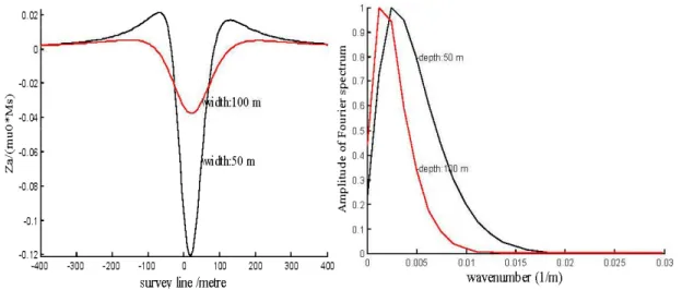
2.3 Magnetic anomaly of a thick prism mo del
The sphere model represents symmetric 3-D body. Many geological bodies can be simplified as an elongated body such as thick prisms, dykes, veins and lenticular etc. One often regards finite extension (or finite depth) geological bodies as an infinite extension (or infinite depth) models, because when length of the thick prism is ten times larger than its depth, the difference in vertical component between the infinite model (Zaoo) and the finite model (Za21) is negligible (Zhining Guan, 2005). Therefore, we considera thick prism as follows (Figure 2.4): its length in the strike direction (y) is infinite. We assume that P is an arbitrary point in space. The equation for the vertical magnetic component Za is expressed as following (Zhining Guan, 2005): (4)
. M2 sin!
tanzs = - - = ,