T
T
H
H
È
È
S
S
E
E
En vue de l'obtention du
D
D
O
O
C
C
T
T
O
O
R
R
A
A
T
T
D
D
E
E
L
L
’
’
U
U
N
N
I
I
V
V
E
E
R
R
S
S
I
I
T
T
É
É
D
D
E
E
T
T
O
O
U
U
L
L
O
O
U
U
S
S
E
E
Délivré par l'Université Toulouse III - Paul Sabatier (UT3Paul Sabatier)Discipline ou spécialité : Génie Civil
JURY
Jean-Paul BALAYSSAC Examinateur Université de Toulouse III Thierry CHAUSSADENT Rapporteur IFSTTAR (HDR) Fabrice DEBY Examinateur Université de Toulouse III
Didier DEFER Examinateur Université d’Artois
Jean-François LATASTE Examinateur Université Bordeaux I Jean SALIN Examinateur EDF R&D
Frédéric SKOCZYLAS Rapporteur Ecole Centrale de Lille Pierre STEPHAN Examinateur EDF R&D
Ecole doctorale : Mécanique, Energétique, Génie civil et Procédés (MeGeP) Unité de recherche : Laboratoire Matériaux et Durabilité des Constructions (LMDC)
Directeur(s) de Thèse : Jean-Paul BALAYSSAC
Co-directeur: Fabrice DEBY
Rapporteurs :
Présentée et soutenue par : Maria Eleni Mitzithra Le 21 Octobre 2013
Titre : Detection of corrosion of reinforced concrete on cooling
THESE
En vue de l’obtention du
DOCTORAT DE L’UNIVERSITE DE TOULOUSE
Délivré par l’Université Toulouse III-Paul Sabatier Discipline ou Spécialité: Génie Civil
Présentée et soutenue par Maria Eleni Mitzithra
le 21 Octobre 2013
Titre: Detection of corrosion of reinforced concrete on cooling
towers of energy production sites
JURY
Jean-Paul BALAYSSAC Examinateur Université de Toulouse III
Thierry CHAUSSADENT Rapporteur IFSTTAR (HDR)
Fabrice DEBY Examinateur Université de Toulouse III
Didier DEFER Examinateur Université d’Artois
Jean-François LATASTE Examinateur Université Bordeaux I
Jean SALIN Examinateur EDF R&D
Frédéric SKOCZYLAS Rapporteur Ecole Centrale de Lille
Pierre STEPHAN Examinateur EDF R&D
Ecole doctorale: Mécanique, Energétique, Génie civil et Procédés (MeGeP) Unité de recherche: Laboratoire Matériaux et Durabilité des Constructions (LMDC) Directeur de thèse: Jean-Paul BALAYSSAC
Abstract
The current thesis is the result of a study funded by Electricité de France –Research and Development (EDF R&D). It aims to develop an original methodology for a better estimation of the state of corrosion of steel reinforced concrete of cooling towers, due to atmospheric carbonation, based on a double approach: the Ground Penetrating Radar (GPR) and the electrochemical measurement of polarization resistance1.
GPR can be used for detecting zones with a high risk of corrosion (detection of contrasts of permittivity). In addition, GPR is used for the location of steel rebars and the estimation of concrete cover thickness.
On the zones identified by GPR with high risk of corrosion, it is proposed to use the polarization resistance measurement to define quantitatively the corrosion activity. This study proposes an original simple operative measurement mode, adapted only for this particular context. After a critical analysis of the existing devices of the polarization resistance measurement, a novel probe is proposed. A numerical model of this probe is developed. Based on the results of the model, abacuses are built in order to gather the real electrochemical proprieties of the steel reinforcement (potential and current) from those values measured on the concrete surface. The role of the influencing factors i.e. physical (injected current, resistivity), geometric (concrete cover, probe’s position) and electrochemical (state of the reinforcement), are fully investigated. The proposed model is applied in a laboratory environment, by reproducing the real site conditions2. The experimental work proves its feasibility, efficiency and effectiveness (within certain limits) by confirming its theoretical principles and indicating some uncertainties during its application. Finally, a primary operational protocol for the on site utilization of the technique is proposed.
Keywords: cooling towers, corrosion, carbonation, GPR, polarization resistance, concrete resistivity, concrete cover, feasibility
1.M.E.Mitzithra, F. Deby, S; Laurens, J. Salin, P. Stephan, D; François, JP Balayssac, Use of an
electrochemical method coupled with ground penetrating radar for the detection of reinforced concrete on cooling towers, 6th International Symposium on Cooling Towers, Cologne, Germany,
June 20-23 2012 , pp 529-537
2 M.E.Mitzithra, F. Deby, S; Laurens, J. Salin, P. Stephan, D; François, JP Balayssac, Numerical
Simulations of a operative measurement mode of polarization resistance adapted for evaluating the corrosion of reinforced concrete on cooling towers, EUROCORR 2012, Istanbul, Turkey, 8-13
Résumé
Cette thèse a été financée par Electricité de France-Recherche et Développement (EDF R&D). L’objectif est le développement d’une méthodologie pour une meilleure estimation de l’état de corrosion des armatures du béton des aéroréfrigérants, soumis à la carbonatation atmosphérique, sur la base d’une double approche: le radar géophysique (GPR) et la mesure de la résistance de polarisation1.
Le GPR peut être utilisé pour la détection rapide des zones présentant un risque élevé de corrosion (détection des contrastes de permittivité). En plus, le GPR est utilisé pour la localisation des armatures d’acier et l’estimation de l’épaisseur d’enrobage. Cette dernière application est très importante pour cette étude.
Dans les zones identifiées comme potentiellement corrodées par le GPR, il est proposé d’utiliser la mesure de la résistance de polarisation pour quantifier l’activité de corrosion. Cette étude propose une méthode opérationnelle et originale, adaptée seulement à cette problématique. Après une analyse critique des dispositifs existants pour la mesure sur site de la résistance de polarisation, un nouveau dispositif est proposé. Un modèle numérique de ce dispositif est développé. Sur la base des résultats du modèle, des abaques sont construites afin de remonter aux propriétés électrochimiques de l’acier (potentiel et courant) à partir des valeurs qui sont mesurées à la surface du béton. Le rôle des paramètres influents, physiques (courant injecté, résistivité), géométriques (enrobage, position de la sonde) et électrochimiques (état de l’acier), est examiné en détail. Ensuite, la méthode d’inversion proposée est testée en laboratoire, sur des corps d’épreuve reproduisant les conditions du site2. La fiabilité et l’efficacité du modèle dans son domaine de définition sont démontrées. Les limites et l’incertitude du protocole de mesure sont également abordées. Enfin, un premier protocole opérationnel pour l’utilisation sur site de la technique est proposé.
Mots clés: aéroréfrigérants, corrosion, carbonatation, GPR, résistance de polarisation, résistivité, enrobage, fiabilité
1. M.E.Mitzithra, F. Deby, S; Laurens, J. Salin, P. Stephan, D; François, JP Balayssac, Use of an
electrochemical method coupled with ground penetrating radar for the detection of reinforced concrete on cooling towers, 6th International Symposium on Cooling Towers, Cologne, Germany,
June 20-23 2012 , pp 529-537
2. M.E.Mitzithra, F. Deby, S; Laurens, J. Salin, P. Stephan, D; François, JP Balayssac, Numerical
Simulations of a operative measurement mode of polarization resistance adapted for evaluating the corrosion of reinforced concrete on cooling towers, EUROCORR 2012, Istanbul, Turkey, 8-13
Acknowledgments
The current PhD thesis which consists part of the national project ANR-Ville Durable-EVADEOS was financed by EDF R&D, in the frame of a contract CIFRE and was carried out in LMDC, INSA-Toulouse, during the period of October 2010 – October 2013. The objective of the thesis was the detection of corrosion of reinforced concrete on cooling towers of energy production stations.
From this position I would like to thank:
Prof. Jean-Paul BALAYSSAC and Dr. Fabrice DEBY (Université de Toulouse III), thesis supervisors, for their substantial support, precious guidance and huge patience during these three years.
Jean SALIN and Pierre STEPHAN (EDF R&D-STEP) for their precious guidance and co-operation during this project.
The Exam Committee, formed by: Prof. Dider DEFER (Université d’Artois) as President of the committee, Prof. Fréderic SKOCZYLAS (Ecole Centrale de Lille), Dr. Thierry CHAUSSADENT (IFSTTAR) and Dr. Jean François LATASTE (Université Bordeaux I).
Special thanks to:
Erwan GALENNE (EDF R&D- CIWAP), for giving me the opportunity to work on this project.
Dr. Stephan LAURENS (INSA Toulouse), for his scientific contribution to the
“kick off” the current thesis.
Pierre-Louis FILLIOT, Antoine De CHILLAZ, Alexandre GIRARD (EDF R&D-STEP) and Prof. Jerôme MARS (ENSE3-Grenoble INP), for their substantial help on the GPR and Signal Processing part of the thesis.
Daniel FRANÇOIS (EDF R&D-STEP), for his scientific contribution during this project.
I woud also like to thank the technical staff of the laboratory for their contribution to the experimental part of the thesis (Sylvain, Bernard, Yann, Carole, Moah...) and the laboratory’s secretariat (Ghislaine, Fabienne..) for their assistance to all administrative matters.
Last but not least, I would like to thank my PhD colleagues, among all: office colleagues (Thomas M., Thomas V., An, Angel, Manh…), Elsa for her substantial
Cédric B. for all the pleasant moments inside and outside the lab during the last hard year of the thesis.
Finally I would like to express my deep gratitude to my family, all my Greek and international friends for their psychological support, comprehension and help during these three years, without them the current PhD thesis would be much more difficult.
Contents
List of figures ... 1 List of tables ... 9 List of symbols ... 11 Abbreviations ... 15 INTRODUCTION ... 171. CONTEXT OF THE STUDY ... 19
2. EDF’s COOLING TOWERS ... 20
3. OBJECTIVES AND STRATEGY DEVELOPMENT ... 23
3.1. Use of a global technique for the localisation of zones exhibiting a potential risk of corrosion ... 24
3.2. Proposal of an original operative local electrochemical technique for the evaluation for the evaluation of corrosion kinetics of the steel rebars embedded in concrete 24 4. OUTLINE OF THE THESIS ... 26
PART A: CORROSION OF REINFORCED CONCRETE: PHENOMENOLOGY AND CHARACTERISATION VIA NON DESTRUCTIVE TECHNIQUES ... 29
I. Corrosion of reinforced concrete: Process and influencing factors ... 29
II. Conventional and alternative techniques for the characterisation of corrosion of reinforced concrete ... 29
III. Ground Penetrating Radar for the location of zones with a high risk of corrosion: Potential of the technique and proposed ameliorations ... 29
I. Corrosion of reinforced concrete: Process and influencing factors ... 31
I.1. INTRODUCTION ... 33
I.2. STEEL CORROSION OF REINFORCED CONCRETE ... 34
I.2.1. Mechanism of steel corrosion ... 34
I.2.2. Kinetics laws of steel corrosion ... 36
I.3. TYPES OF STEEL CORROSION OF REINFORCED CONCRETE ... 38
I.3.1. Uniform corrosion: phenomenon of carbonation ... 39
I.3.2. Penetration of chloride ions ... 42
I.4. CONCLUSION ... 43
II. Conventional and alternative techniques for the characterisation of corrosion of reinforced concrete ... 45
II.1. INTRODUCTION ... 47
II.2. CONVENTIONAL TECHNIQUES FOR DETECTING STEEL CORROSION OF REINFORCED CONCRETE STRUCTURES... 48
II.2.1. Electrical resistivity of concrete ... 48
II.2.2. “Half cell” potential measurements ... 51
II.2.3. Linear Polarisation Resistance Measurement ... 53
II.2.3.1. Definition ... 53
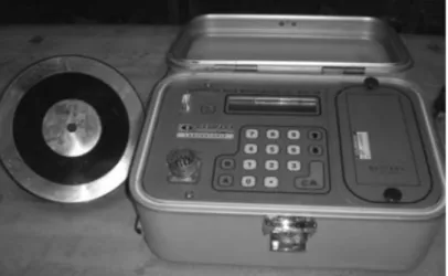
II.2.3.2. Measurement instruments of linear polarisation resistance ... 55
II.2.4. Electrochemical Impedance Spectroscopy-EIS ... 60
II.2.5. Synthesis ... 62
II.3. ALTERNATIVE TECHNIQUES FOR THE CHARACTERISATION OF CORROSION OF REINFORCED CONCRETE STRUCTURES... 64
II.3.2. Infra Red thermography ... 68
II.3.3. Synthesis ... 69
II.4. CONCLUSION ... 71
III. Ground Penetrating Radar for the location of zones with a high risk of corrosion: Potential of the technique and proposed ameliorations ... 73
III.1. INTRODUCTION ... 75
III.2. USE OF GPR IN CIVIL ENGINEERING ... 76
III.2.1. Basic Principle of GPR for the auscultation of reinforced concrete structures 76 III.2.2. Electromagnetic properties of concrete ... 77
III.2.3. Influence of humidity on the electromagnetic concrete properties and the propagation of GPR waves ... 78
III.2.3.1. Influence of humidity of the effective permittivity of concrete ... 78
III.2.3.2. Influence of humidity on the amplitude and the speed of GPR direct wave 79 III.2.4. Methods for measuring the propagation velocity of the GPR waves ... 80
III.2.4.1. WARR and CMP methods ... 80
III.2.4.2. FO method ... 81
III.2.5. Synthesis ... 82
III.3. EXAMPLES OF THE TECHNIQUE RADAR FOR THE RESEARCH OF ZONES WITH HIGH POTENTIAL OF RISK OF CORROSION ... 84
III.3.1. General Principle of evaluating the risk of corrosion via radar ... 84
III.3.2. Examples of GPR application for the location of zones in risk of corrosion 85 III.3.3 Synthesis ... 89
III.4 SIGNAL PROCESSING FOR SOLVING THE PROBLEMS ENCOUNTERED DURING THE ON SITE APPLICATION OF RADAR ... 90
III.4.1. Wiener and Median Filter (GIPSA Lab) ... 92
III.4.2. Subtraction of the direct signal from the mixed signal (LMDC) and Singular Value Decomposition (SVD) (EDF R&D-STEP) ... 97
III.4.3. Example of calculation of concrete cover thickness after signal processing with subtraction of the direct signal or SVD ... 100
III.4.4. Synthesis ... 102
III.5. CONCLUSION ... 103
PART B: DEVELOPMENT AND VALIDATION OF A PROTOCOL FOR THE POLARISATION RESISTANCE MEASUREMENT ... 107
IV. Problems of the polarisation resistance measurement: State of the art .. 107
V. Proposal of a novel operative measurement mode of polarisation resistance 107 VI. Experimental validation of the proposed operative polarisation resistance measurement mode ... 107
IV. Problems of the polarisation resistance measurement: State of the art ... 109
IV.1 INTRODUCTION ... 111
IV.2 STATE OF THE ART ... 111
IV.3. SYNTHESIS ... 117
IV.4. CONCLUSION ... 121
V. Proposal of a novel operative measurement mode of polarisation resistance 123 V.1. INTRODUCTION ... 125
V.2. PROPOSAL OF AN ALTERNATIVE METHODOLOGY FOR THE POLARISATION RESISTANCE MEASUREMENT ... 125
V.1.1. Synthesis ... 129
V.3. NUMERICAL SIMULATIONS OF THE NOVEL PROBE PROPOSED FOR THE POLARIZATION RESISTANCE MEASUREMENT ... 131
V.3.1. Geometry definition ... 131
V.3.2. General properties, electro-kinetics equations and boundary conditions of the model 134 V.3.3. Distribution of the injected current lines in the simulated geometries .. 135
V.3.4. Current density and potential distribution along the reinforcement of the simulated geometries ... 139
V.3.4.1. Influence of resistivity, concrete cover, size of the counter electrode and injected current on the current density and potential distribution ... 140
V.3.4.2. Influence of the reinforcement state on the current density and potential distribution ... 146
V.3.4.3. Influence of the different reinforcement configurations on the current density distribution ... 151
V.3.4.4. Influence of probe’s position on the current density distribution .. 154
V.3.5. Synthesis ... 155
V.4. SENSITIVITY OF THE POLARISATION RESISTANCE MEASUREMENT TO ITS INFLUENCING PARAMETERS VIA NUMERICAL APPROACH: DESIGN OF EXPERIMENTS (DOE) ... 157
V.4.1. Experiment design for the estimation of the potential, Eαr, on the active steel rebar right under the measurement point ... 158
V.4.2. Experiment design for the estimation of the current density, jαr, on the active steel rebar right under the measurement point ... 162
V.4.3 Synthesis ... 165
V.5. CALCULATION OF POLARISATION RESISTANCE ON THE SURFACE OF STEEL REBAR REINFORCEMENT AND CONSTRUCTION OF ABACUSES 167 V.5.1. Correction laws and abacuses for a single active rebar ... 167
V.5.2. Correction laws and abacuses for a single passive rebar ... 172
V.5.3. Correction laws and abacuses for the two crossed-rebar configuration. 175 V.5.4. Synthesis ... 177
V.6. CONCLUSION ... 178
VI. Experimental validation of the proposed measurement mode of polarisation resistance ... 181
VI.1. INTRODUCTION ... 183
VI.2. EXPERIMENTAL PROGRAM ... 183
VI.2.1. Specimens’ preparation ... 183
VI.2.2. Materials’ composition ... 186
VI.2.3. Synthesis ... 188
VI.3. DETERMINATION OF ELECTROCHEMICAL PARAMETERS ... 190
VI.3.1. Experimental procedure and set up ... 190
VI.3.2. JoRΩ Correction ... 192
VI.3.3 Evaluation of parameters of Butler Volmer equation ... 195
VI.3.4. Synthesis ... 197
VI.4. DETERMINATION OF THE CORROSION CURRENT DENSITY OF THE STEEL REBARS ... 198
VI.4.1. Experimental procedure and set up ... 198
VΙ.4.2. Demonstration of the proposed polarisation resistance measurement model: Validation of the feasibility of the technique ... 204
VI.4.2.1 Evaluation of the potential and current density on the steel rebar
surface after polarisation ... 205
VI.4.2.2. Calculation of polarization resistance and corrosion current density values 208 VI.4.2.3. Anodic aspect of the polarization resistance measurement ... 210
V.4.2.4 The aspect of time in polarization resistance measurement: Polarization and De-polarization duration ... 212
VI.4.2.4 Synthesis ... 213
VI.4.3. Application of the proposed polarisation resistance measurement model: Estimation of the corrosion current density of the reinforcement ... 215
VI.4.3.1. Results obtained with slab I-C ... 215
VI.4.3.2. Results obtained with slab I-C: Reactivation of corrosion ... 221
VI.4.3.3. Relation between polarization resistance-resistivity and polarization resistance-corrosion potential ... 223
VI.4.3.4. Results obtained with slab I-NC ... 225
VI.4.3.5. Results obtained with slab II-C ... 227
VI.4.3.6. Synthesis ... 229
VI.4.4. Uncertainty of the proposed polarisation resistance measurement model: tests of repeatability and spatial variability ... 229
VI.4.4.1. Repeatability test ... 230
VI.4.4.2. Spatial variability test ... 232
VI.4.4.3. Synthesis ... 235
VI.4.5. Determination of weight losses due to corrosion and calculation of corrosion current density by Faraday law ... 236
VI.4.5.1. Weight loss of steel rebars calculated according to Faraday’s law 236 VI.4.5.2. Weight loss of steel rebars measured via a gravimetric technique vs. weight loss estimated via Faraday’s law ... 241
VI.4.5.3. Synthesis ... 243
VI.5. CONCLUSION ... 244
CONCLUSIONS AND PERSPECTIVES ... 247
BIBLIOGRAPHY ... 255
APPENDIX A ... 265
APPENDIX B ... 273
B.1. Specimens’ fabrication and conditioning... 275
B.2. Mechanical and physical characteristics of casted concrete ... 280
B.3. Synthesis ... 281
List of figures
Figure 0. 1: Cooling towers (shell, piles and foundations) of nuclear power stations. 20 Figure 0. 2: Schematic illustration of cooling towers (F. Coppel, 2009).. Moving from the top and downwards: cap, saddle, lintel and tread. (Eiffage, 2009). ... 21
Figure I. 1: Schematic representation of steel corrosion process in the basic environment (Gulikers, 2005). ... 35 Figure I. 2: Graph of η against log(j) for both electrode processes during corrosion. Straight lines are traced with a slope equal to the respective β-constant. The intersection defines the system’s equilibrium (no current flow): the corrosion potential, Ecorr, and the corrosion current density, jcorr. ... 38
Figure I. 3 : Carbonation front via the phenolphthalein technique. The transparent sides are attributed to the carbonation (ME Mitzithra, 2008). ... 40 Figure I. 4.:Electrochemical behaviour of active and passive steel bars acting as independent electrochemical systems. (A.Nasser, 2010). ... 41 Figure I. 5: Electrochemical behaviour of active and passive steel bars after electrical connection (coupled electrochemical system) (A.Nasser, 2010). ... 43
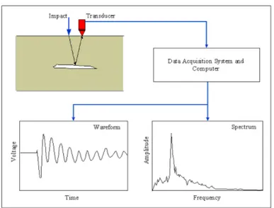
Figure II. 1: Set up of four electrodes measurement of concrete resistivity (R.Polder, 2001). ... 48 Figure II. 2: Principle and main components of half cell potential measurements: Reference electrode, high impedance voltmeter, connection to the rebar (R.B. Polder, 2001) ... 51 Figure II. 3: Examples of half-cell potential maps (Riding dick in the Tunnel San Berardino) in a colour plot (right) and equicontour line plot (left) (C.Andrade, 2004). ... 52 Figure II. 4.: Polarisation curve describing the Butler-Volmer model. (Luping, 2002). ... 54 Figure II. 5: The GECOR 6 corrosion Rate Meter developed in Spain (D.Macdonald,2009). ... 55 Figure II. 6: GECOR 6 electrodes’ configuration (Nygaard, 2009). ... 56 Figure II. 7: Polarisation of reinforcement according to GECOR 6.(Nygaard,2009). . 57 Figure II. 8: The Galvapulse instrument from FORCE Technology (Denmark) (Nygaard,2009) ... 57 Figure II. 9: Randles circuit and the response to a short galvanostatic pulse (S.Laurens, 2010) ... 58 Figure II. 10: Galvapulse electrodes configuration (Nygaard, 2009) ... 58 Figure II. 11: Ershler-Randles equivalent circuit for a charge transfer reaction at an electrode surface. (B.E.Conway,1999). ... 61 Figure II. 12: Principle of ultrasonic testing. (BS EN 583-2:2001). ... 66 Figure II. 13: Schematic simplified representation of the impact echo method (Sansalone, 1998). ... 67 FigureII. 14: Schematic representation of tomographic transmission measurements . 68 Figure II. 15: Principle of infra red thermography ... 69
Figure III. 1: Principle of radar measurement in reinforced concrete (K.Viriyametanont, 2008) 76
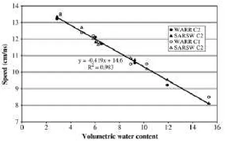
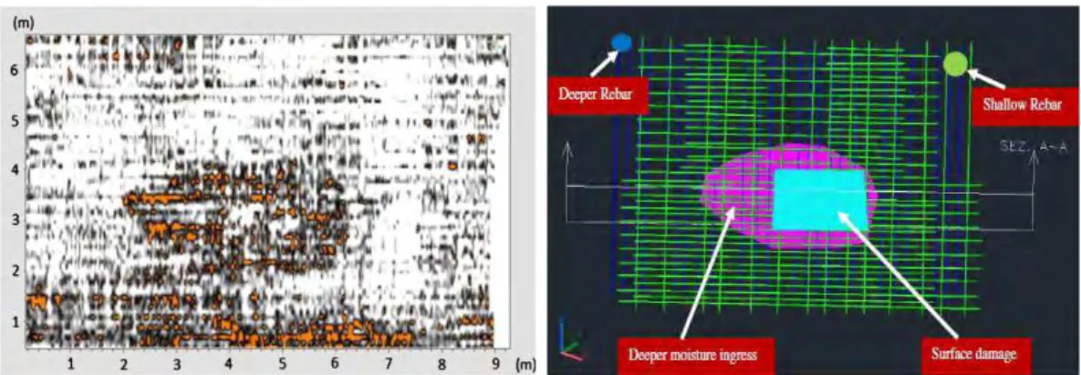
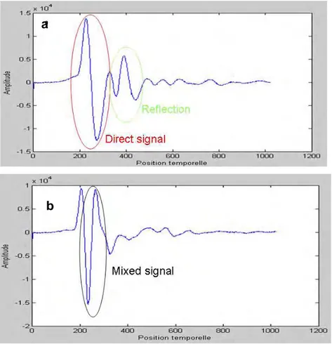
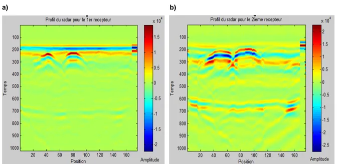
Figure III. 2: Effect of water volume (%) on the relative permittivity and conductivity of concrete for a frequency of 500 MHz (Soutsos et al, 2001) ... 78 Figure III. 3.: a) Direct wave of GPR antenna in concrete (Z.M.Sbartai, 2007) b) Relation between the peak to peak amplitude of the direct wave and the water volume (%) in different concretes (K.Viriyametanont, 2008) ... 79 Figure III. 4. Variation of the direct wave velocity as a function of the water content in concrete (G.Klysz, 2007) ... 80 Figure III. 5: Arrival time of the direct and reflected wave as a function of the distance between transmitter-receiver (G.Klysz, 2004) ... 81 Figure III. 6: Schematic illustration of the different methods used for measuring the propagation velocity of GPR signals. ... 82 Figure III. 7: GPR scanned area of Forth Road Bridge detecting different rebar layers on a longitudinal section (depth against distance) (A.Alani et al, 2013) ... 85 Figure III. 8: Area with increased attenuation (left) and schematic 3D drawing with AutoCAD indicating the zones of high moisture penetration (right) of the Forth Road Bridge, Edinburgh, Scotland (A .Alani et al, 2013). ... 85 Figure III. 9: Examples of ICR and corrosion potential mappings for two different a) and b) concrete bridge decks. (S. Laurens, 2001) ... 86 Figure III. 10: GPR scanning along the reinforced concrete beam.. ... 87 Figure III. 11: Peak to peak amplitude mapping of the GPR direct signal of one of the sides of the reinforced concrete beam. ... 88 Figure III. 12: A-scan of GPR signal propagated in concrete structure with steel rebars embedded at a) >5cm and b) <3cm. ... 91 Figure III. 13: Dry sand box of 1x 1 x 0.3m, where smooth rounded steel rebars (ø 16mm)-indicated by the red arrow were embedded at 2.2 cm.. ... 92 Figure III. 14: Radar profiles with highly mixed signals (direct wave and reflection of the steel rebars embedded in the dry sand at 2.2cm and with a spacing of 20cm for a) 1st and b) 2nd receiver of GPR. ... 93 Figure III. 15: Direct signal after the application of Wiener filter for the steel rebars embedded in the dry sand at 2.2cm and with a spacing of 20cm for a) 1st and b) 2nd receiver of GPR... 93 Figure III. 16: Reflected signal from the steel rebars after the application of Wiener filter for the steel rebars embedded in the dry sand at 2.2cm and with a spacing of 20cm for a) 1st and b) 2nd receiver of GPR ... 94 Figure III. 17: Radar profiles (B-scans) for the steel rebars with a spacing at 40cm, embedded at 2.2cm in the dry sand, for the a) 1st and b) the 2nd receiver.. ... 94 Figure III. 18: Direct signal after the application of Wiener filter for the steel rebar embedded in the dry sand at 2.2cm with a spacing of 40cm for a) 1st and b) 2nd receiver of GPR... 95 Figure III. 19: Reflected signal from the steel rebars after the application of Wiener filter for the steel rebar embedded in the dry sand at 2.2cm with a spacing of 40cm for a) 1st and b) 2nd receiver of GPR ... 95 Figure III. 20: Direct signal after the application of Median filter for the steel rebar embedded in the dry sand at 2.2cm with a spacing of 40cm for a) 1st and b) 2nd receiver of GPR... 96 Figure III. 21: Reflected signal from the steel rebars after the application of Wiener filter for the steel rebar embedded in the dry sand at 2.2cm with a spacing of 40cm for a) 1st and b) 2nd receiver of GPR ... 96 Figure III. 22: a) Wall I-N (EDF power plant, Le Havre). b) II-NC reinforced concrete slab casted in LMDC (see also §VI.2.1. and §VI.2.3).. ... 98
Figure III. 23: a) GPR profile along the wall I-N (EDF power plant, le Havre) for the 1st receiver. b) Signals before and after SVD, for the hyperbole indicated in III.23.a) ... 98 Figure III. 24: a) Hyperbolic zone (see also figure III.23) with mixed signal b) Reflected signal of the steel rebar after the subtraction of the direct signal. ... 99 Figure III. 25: Signals for the summit (exact position f the steel rebar) of the hyperbole a) mixed signal b) direct signal after the subtraction c) reflected signal from the steel rebar after the subtraction ... 99 Figure III. 26: Estimation of concrete cover, h(cm), according to Pythagora’s law and equations (eq. 41) and (eq. 42). ... 100 Figure III. 27: a) Radar profiles on the II-NC reinforced concrete slab, fabricated in LMDC.. b) Separation of signals after SVD for the summit of the hyperbole indicated at figure III.26.. ... 101
Figure IV. 1. Schematic illustration of the current, I’CE, flowing to the reinforcement over the assumed confinement length, L’CE, and the length LCE over which the applied counter electrode current, ICE, is distributed. A current IGE is applied from the guard ring for confining the counter electrode current, ICE. (Nygaard, 2009) 112 Figure IV. 2: Schematic illustration of self confinement. (Nygaard, 2009). ... 113 Figure IV. 3: Illustration of the «overconfining» occurring at high corrosion activity of rebar during measurements with the modulated GE. (Wojtas, 2004) ... 114 Figure IV. 4: Current density mapping of the steel area assumed to be polarised according to RILEM recommendations. (S. Laurens, 2010). ... 115 Figure IV. 5: Numerical simulations of GECOR6 measurement: (S.Laurens, 2010). ... 116
Figure V. 1: Qualitative schematic representation of the proposed measurement
polarization technique………. 128
Figure V. 2: Schematic illustration of probes for: a) LMDC simulated model; b) Galvapuse (Laurens, 2010);c) Gecor6 (Laurens, 2010). Dimensions in mm. ... 132 Figure V. 3: Geometry of the simulated reinforced concrete specimens with: a) a single steel rebar embedded at 6cm and the probe placed above the middle of the single bar b) two crossed rebars-the top embedded at 6cm and the probe placed above the crossing of the rebars. ... 133 Figure V. 4: Geometry of the simulated reinforced concrete specimens with: a) ) two crossed rebars-the top embedded at 6cm and the probe above the crossing of the rebars b) the same reinforcement configuration and the probe placed above the middle of the reinforcement mesh ... 133 Figure V. 5: Coarse mesh applied on the concrete volume with a single steel rebar embedded at 1cm.. ... 135 Figure V. 6: Injected current density lines (ICE=50µA) for the geometry with one
single bar at active state, for concrete resistivity of 2000 Ohm m, embedded at a)1cm and at b)6cm and the probe placed above the middle of the single bar. The colour bar gives the potential range (V). ... 136 Figure V. 7: Injected current density lines (ICE=50µA) for the geometry with one
single bar embedded at 6cm at a) active state) and b) at passive state for concrete resistivity of 2000 Ohm m and the probe placed above the middle of the single bar. The colour bar gives the potential range (V). ... 136 Figure V. 8: Injected current density lines (ICE=50µA) for the geometry with a) a
middle of the single bar ,b) two crossed rebars at active state-the top embedded at 6cm and the probe placed above the crossing of the rebars c) a network of 4 rebars at active state–the top ones embedded at 6cm- and the probe above one of the crossing of the rebars. The concrete resistivity is 2000 Ohm m. The colour bar gives the potential range (V). ... 137 Figure V. 9: Injected current density lines (ICE=50µA) for the geometry with two
crossed rebars at active state-the top embedded at 6cm and the probe placed a) above the crossing of the rebars, b) at a distance of 11.9cm from the upper rebar and 9.4 cm from the lower rebar, right on the concrete specimen’s surface. The concrete resistivity is 2000 Ohm m. The colour bar gives the potential range (V). ... 137 Figure V. 10: Indication (in red) of the fibre under investigation towards polarisation for two bars configuration. ... 139 Figure V. 11: Indication (in red) of the “point of interest” on the steel rebar right under the measurement point on the surface of the concrete specimen. ... 140 Figure V. 12: Current density distribution along the steel bar for the single bar configuration in active state for every value of injected current from the probe with e=6 cm and a) ρ=50 Ohm m and b) ρ=2000 Ohm m. ... 141 Figure V. 13: Potential distribution along the steel bar for the single bar configuration, in active state, for every value of injected current from the probe with e=6 cm and a)
ρ=50 Ohm.m and b) ρ=2000 Ohm.m. ... 143
FigureV. 14: Current density distribution along the steel bar for the single bar configuration in active state, for every value of injected current from the probe with
ρ=50 Ohm.m, a) e=1 cm and b) e=6 cm. The probe’s position along the steel rebar
(x-axis) is also indicated. ... 144 Figure V. 15: Current density distribution along the steel bar for the single bar configuration in active state, for every value of injected current from the probe with
ρ=50 Ohm.m and e=6 cm. ... 145
Figure V. 16: Potential distribution along the steel bar for the single bar configuration, in active state, for every value of injected current from the probe with ρ=50 Ohm.m, a) e=1cm and b) e=6cm (under). ... 146 Figure V. 17: Current density distribution along the steel bar for the single bar configuration for every value of injected current from the probe with ρ=2000 Ohm.m and e=6 cm in a) active and b) passive state. ... 147 Figure V. 18: Potential distribution along the steel bar for the single bar configuration, for every value of injected current from the probe with ρ=2000 Ohm.m, e=6cm, in a) active state and b) passive state. ... 148 Figure V. 19: Polarisation measurement: Qualitative representation of potential shift,
∆Ε, due to current shift, ∆i, along the Butler Volmer curves for: a) active steel rebar
b) passive steel rebar ... 149 Figure V. 20: Anodic polarisation curve for the steel bar (on the “point of interest”) for the single bar configuration, for every value of injected current from the probe with ρ=2000 Ohm.m, e=6cm, in a) active state and b) passive state. ... 150 Figure V. 21: Current density distribution along the active steel bar for every value of injected current from the probe with ρ=2000 Ohm.m and e=6 cm for a) a single bar and b) two crossing rebars configuration. ... 151 Figure V. 22: Current density losses (%) on the active steel rebar, right under the measurement point on the concrete surface, between the single and two bars configuration for every injected current and resistivity, for a) e=1cm and b) e=6cm. ... 152
Figure V. 23: Current density losses (%) on the active steel rebar, right under the measurement point on the concrete surface, between the single and four bars configuration for every injected current and resistivity, for a) e=1cm and b) e=6cm. ... 153 Figure V. 24: Current density distribution along the upper active steel bar for every value of injected current from the probe with ρ=2000 Ohm m and e=6 cm for the probe placed a) above the crossing of the rebars and b) at a distance from the crossed rebars. ... 155 Figure V. 25: Potential response, Ear, (V) of each numerical experiment vs. potential
Ẻar (V) predicted from the statistical model. ... 160
Figure V. 26: Quadratic surface model for the potential response, Ẻar (V) as a function
of resistivity, injected current and corrosions current density. βaa ; βac, and e are fixed
at 0.2 V/dec, 0.1 V/dec and 3cm respectively. The black points correspond to the CCC design. ... 162 Figure V. 27: Current density response, jar, (A/m2) of each numerical experiment vs.
potential ĵar (A/m2) predicted from the statistical model ... 164
Figure V. 28: Quadratic surface model for the current density, ĵar (A/m2) as a function
of resistivity, injected current and anodic Tafel constant. jcorr, βac, and e are fixed at
0.005A/m2, 0.1 V/dec and 3cm respectively. The black points correspond to the CCC design. ... 165 Figure V. 29: Ohmic drop versus resistivity for every injected current from the probe towards a single active steel rebar, embedded at a) 1cm and b) 6 cm, with the probe above the middle of the single bar. ... 168 Figure V. 30: Abacus of coefficient k as a function of concrete cover for a) 1-5-10 µA and b) 20-30-50µΑ of the injected current from the probe towards a single active steel rebar. Region with reduced efficiency of the abacus is noted in red. ... 169 Figure V. 31: Ln(jarr/iCE) versus concrete cover for each concrete resistivity and for an
injected current of a)1 and b) 50µΑ, towards the single active steel rebar, with the probe above the middle of the single bar. ... 171 Figure V. 32: Abacus of coefficients A and B as a function of concrete resistivity, for a single active steel rebar. ... 172 Figure V. 33: Ohmic drop versus resistivity for every injected current from the probe towards a single passive steel rebar, embedded at 6 cm with the probe above the middle of the single bar... 173 Figure V. 34: Abacus of coefficient k as a function of concrete cover for each injected current from the probe towards a single passive steel rebar. ... 173 Figure V. 35: jar/iCE versus concrete cover for each concrete resistivity and for an
injected current of 50µΑ towards the single passive steel rebar, with the probe above the middle of the single bar. ... 174 Figure V. 36: Abacus of coefficient a as a function of concrete resistivity, for a single passive steel rebar ... 175 Figure V. 37: Abacus of coefficient b as a function of concrete resistivity, for a single passive steel rebar. ... 175 Figure V. 38: Abacus of coefficient k as a function of concrete cover for each injected current from the probe towards one single active rebar (full line) and two crossed active steel rebars (doted line). ... 176 Figure V. 39: Abacus of coefficients A and B as a function of concrete resistivity, for one single active rebar (full line) and two crossed active steel rebars (doted line). .. 177 Figure V. 40: Schematic illustration of the procedure, calculating the real value of polarisation resistance for an active or passive rebar... 178
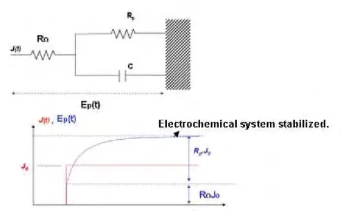
Figure VI. 1: Schematic illustration of concrete slabs of a) single bar configuration (Type I) and b) two crossed rebar configuration (Type II)………. 184 Figure VI. 2: Schematic illustration of the top view of the concrete slabs of a) single bar configuration (Type I) and b) two crossed rebar configuration (Type II). PVC hooves are marked with red colour. ... 184 Figure VI. 3: PVC hooves used for eliminating any possible undesirable influence of the environment on the state of the reinforcement... 185 Figure VI. 4: Schematic illustration of the electrical connection between the steel rebars and the polarisation resistance measurement system. ... 185 Figure VI. 5: Schematic illustration of the matrix used for the reinforced concrete specimen, intended for measuring Tafel constants. ... 186 Figure VI. 6: Steel rebar after cleaning it with acetone and ethanol to remove the grease and before embedding it into the concrete. No mechanical treatment was carried out. ... 187 Figure VI. 7: Preparation and storage conditions chart flow of the concrete slabs and specimens, followed for both types of concrete... 190 Figure VI. 8: Cylindrical reinforced concrete specimen, used for the Tafel constant measurements ... 191 Figure VI. 9: Schematic illustration and picture of the experimental set up for the Constant Tafel measurements. ... 191 Figure VI. 10: Sweep polarisation curve plotted during the Tafel measurement for an active (carbonated) concrete specimen ... 192 Figure VI. 11: Potential response of an active system to a short galvanostatic pulse of 10µA.The OC or corrosion potential is firstly measured till stabilisation. EΩ(V) is the
instantaneous response of the system, due to the ohmic resistance of concrete, according to Randles model see figure II.9). ... 193 Figure VI. 12: Tafel curves for a) an active (carbonated) and b) passive (carbonated) type II concrete specimen before and after JoRΩ correction. ... 194
Figure VI. 13: Experimental Tafel and fitted-in curve for an active (carbonated) specimen.. ... 195 Figure VI. 14: Successive positions of Wenner probe for measuring concrete resistivity. ... 199 Figure VI. 15: Measurement of concrete resistivity on the slabs via the technique of Wenner.. ... 199 Figure VI. 16: Experimental set up of the3 electrode polarisation resistance measurement, on one single point on the concrete surface of the slab, placed, right above the steel rebar: the stainless steel counter electrode (CE), the SCE reference electrode (RE). ... 200 Figure VI. 17: OC or corrosion potential measurement taking place above the crossing of the two rebars at an active state, with a concrete cover of 2cm (type II carbonated (C)).. ... 202 Figure VI. 18: Polarisation measurement taking place above the crossing of the two rebars at an active state, with a concrete cover of 2cm (type II carbonated (C)). ... 202 Figure VI. 19: Procedure of corrosion potential and polarisation measurement ... 203 Figure VI. 20: Polarisation measurements above the middle of the single steel rebar (type I), the crossing and a point between the crossing and one of the edges of the upper steel rebar (type II). ... 204 Figure VI. 21: Calculating Ear (V) according to procedure described in §V.5.1 after
Figure VI. 22: Calculating jar (A/m2) according to procedure described in §V.5.1 after
injecting 50µA. ... 207 Figure VI. 23: Polarisation (∆Ep(V) vs. ja (A/m2)) curve at Ecorr for polarisation
resistance measurement on the active steel rebar embedded at 2cm. ... 208 Figure VI. 24: Polarisation (∆Ep(V) vs. jar (A/m2)) Curve at Ecorr for polarisation
resistance measurement on the passive steel rebar embedded at 2cm. The slope of this curve represents the Rp value (Ohm m2) of the steel rebar ... 210
Figure VI. 25: Schematic illustration of the procedure, calculating the real value of polarisation resistance for an active or passive rebar... 212 Figure VI. 26: Average concrete resistivity for I-C slab in July and October 2012 (a), corrosion potential values (before any polarisation) (b) for the steel rebar at 2 and 5cm. The slab had already been removed from the carbonation in June 2012, and from July till October, it was preserved in the laboratory ambiance. ... 216 Figure VI. 27: a) Polarisation resistance and b) corrosion current density values for the active steel rebars embedded at 2 and 5cm, measured at two different periods (July and October 2012)... 219 Figure VI. 28: a) Polarisation resistance and b) corrosion current density values for the embedded rebars at 2 and 5cm, measured at the same period (October 2012), treated as active and apparent “passive” rebars). ... 220 Figure VI. 29: a) Average concrete resistivity for I-C slab in July, October 2012 and January 2013, b) corrosion potential values (before any polarisation) for the steel rebar at 2 and 5cm. The slab was already removed from the carbonation chamber in June 2012, and from July till October 2012, it was preserved in the laboratory ambiance. In the end of November 2012, the slab was stored for 45 days in the chamber of fixed temperature (20oC) and humidity (95%). ... 222 Figure VI. 30: Polarisation resistance values for the embedded rebars at 2 and 5cm, measured on July, October 2012 and January 2013. ... 222 Figure VI. 31: Corrosion current density values for the embedded rebars at 2 and 5cm, measured in July, October 2012 and January 2013. ... 223 Figure VI. 32: Polarisation resistance Rp, plotted vs. Concrete resistivity, ρ. ... 224 FigureVI. 33 : Polarisation resistance Rp, plotted vs. Corrosion potential, Ecorr ... 224
Figure VI. 34: a) Average concrete resistivity for the I-C and I-NC concrete slab and b) corrosion potential values for the embedded rebars at 2 and 5cm (b), measured in October 2012. ... 225 Figure VI. 35: Polarisation resistance, Rp, (a) and corrosion current density, jcorr, (b)
values for the embedded rebars at 2 and 5cm, in the C and NC slabs, measured in October 2012. The value of injected current for which the polarisation-target of 20mV±3mV was achieved is also given for each measurement. ... 226 Figure VI. 36: Corrosion potential values for two different points (a and b) of measurement on the upper steel rebar embedded at 2 and 5cm. ... 227 Figure VI. 37 : a) Polarisation resistance and b) corrosion current density values for two different points (a and b) of measurement on the upper steel rebar embedded at 2 and 5cm ... 228 Figure VI. 38: Spatial variability test on the rebars embedded at 2 and 5cm of the I-C concrete slab in October 2012... 232 Figure VI. 39: Variation (%) of jcorr regarding position 0 of the probe for the steel
rebar embedded at a) e=2cm and b) e=5cm in I-C concrete slab. ... 235 Figure VI. 40: Monitoring of the a) concrete resistivity of the slab and b) corrosion potential for the rebars embedded at 2 and 5cm. The measurement lasted 61 days. . 238
Figure VI. 41: Monitoring of a) polarisation resistance b) and corrosion current density for the rebars embedded at 2 and 5cm. The measurement lasted 61 days. ... 239 Figure VI. 42: Weight loss of steel rebars at 2cm and 5 cm in the I-C2 concrete slab, calculated according to Faraday’s law after a monitoring of the corrosion current during 61 days. ... 240 Figure VI. 43: Steel rebar right after its recovery from the I-C2 slab, where corrosion products are a) still on and b) right after the removal of these products, according to the instruction of the European Standards ISO 8407:2009. ... 241 Figure VI. 44: Weight loss of the steel rebars embedded at 2 and 5cm for the I-C2 concrete slab estimated via Faraday’s law and measured after being recovered from the concrete slab. ... 242 Figure VI. 45: A first version of a complete protocol of measuring polarisation resistance on a single point on reinforced concrete cooling towers of energy production sites ... 246
Figure A. 1: Fractional CCC design of resolution V for 6 factors. (W. Tinsson,
2010)……….. 267
Figure B. 1: Casting of the reinforced concrete slabs and specimen 275 Figure B. 2:24h curing of the concrete specimens in a chamber of fixed temperature (20°C) andrelative humidity (95°C). ... 276 Figure B. 3: a) Reinforced concrete slab) and b) cylindrical specimen before storing in the chamber of accelerated carbonation (50%CO2, 60% RH). Their sides are
covered with self-adhesive Al paper. ... 277 Figure B. 4: Chamber of accelerated carbonation (50%CO2, 60%.RH) ... 277
Figure B. 5: a) Reinforced concrete slab and b) cylindrical specimen entirely covered with auto adhesive Al paper, in order to avoid any undesirable corrosion from environmental conditions. ... 278 Figure B. 6: Concrete specimen for control of carbonation. Controlling the ingress of carbonation with phenolphthalein after one month (right) and two months (left). .... 279 Figure B. 7: Concrete specimen for control of carbonation. Carbonation ingress tested with phenolphthalein after one month (right) and two months (left). Violet colour indicates that the specimen is not carbonated. ... 279 Figure B. 8: Pore size distribution according to Hg porosimetry for the concrete type I (1 single rebar configuration), carbonated (blue curve) and non carbonated (pink curve). The curves are highly disturbed due to the measurement’s noise. ... 281 Figure C. 1: Successive positions of Wenner probe for measuring concrete resistivity, indicated by the black arrows of the formed square. A point is fixed in the middle of the square and the probe is placed as indicated by the red arrows. 287
Figure C. 2: Procedure of corrosion potential and polarisation measurement ... 291 Figure C. 3: a) Definition of measurement zones .. b). Potentiostat GAMRY Ref. 600 of 1 channel, equipped with a laptop for measurement settings and data processing. c). Experimental set up and electrodes’ configuration during the polarisation resistance measurement. ... 293 FigureC. 4 : Procedure of calculating, the potential, Ear (V) and the current density; iar
(A/m2) on the steel rebar. ... 294 FigureC. 5: Polarisation (Ear(V) vs. jar (A/m2)). ... 295
List of tables
Table II- 1: Concrete resistivity and risk of reinforcement corrosion at 20°C for OPC concrete (R.B. Polder, 2001) ... 50 TableII- 2: Corrosion potential and risk of reinforcement corrosion at 20°C for OPC concrete (J.P.Broomfield, 1997)), (Cox, 1997) ... 53 Table II- 3: Characteristics of GECOR 6 and Galvapulse ... 59 Table II- 4: Correlation between corrosion classification and corrosion current density (D.W. Law, 2004) ... 60 Table II- 5: Advantages and Disadvantages of the conventional techniques used for the evaluation of the reinforcement corrosion ... 63 Table II- 6: Advantages and Drawbacks of the alternative techniques used for the general evaluation of the condition of a structure ... 70 Table III- 1: Influence of humidity on the electromagnetic properties of concrete and
characteristics of direct wave 83
Table III- 2: Advantages and disadvantages of the methods for measuring the propagation velocity of direct wave of GPR. E: is the emitter and R is receiver of the electromagnetic signal ... 83 Table III- 3: Overview of examples of GPR applied for the research of zones with a potential of risk of corrosion ... 90 Table III- 4: Errors of the techniques SVD and subtraction of the direct signal on the estimation of concrete cover ... 102 Table III- 5: Techniques tested in the frame of the current study for the separation of mixed signals (direct and reflected wave) due to the dense reinforcement network of real reinforced concrete structures ... 103 Table IV- 1: Review: On-site polarisation resistance measurement with GECOR6 and Galvapulse 118
Table V- 1: A primary comparison between GECOR6, Galvapulse and the proposed Rp measurement model 130
Table V- 2: The Butler- Volmer parameters implemented in the model ... 134 Table V- 3: Influence of physical ad geometrical parameters on the polarisation of the “point of interest” according to the proposed measurement model ... 156 TableV- 4 : Ranges of values for the factors influencing the potential response, Ea, (V), on the active steel rebar for the single bar configuration ... 158 Table V- 5: Estimators, Standard deviation, t and p-values for each parameter. ... 159 Table V- 6: Estimators, Standard deviation, t and p-values for each parameter. ... 163 Table V- 7: The 4 most significant parameters influencing the responses Ear and jar
respectively ... 166
Table VI- 1: Concrete formulation………. 187
Table VI- 2: Water absorption by the aggregates (NF EN 1097-6) ... 187 Table VI- 3: Details about the characterisation of concrete’s mechanical and physical properties and the number of concrete specimen (SP), for each technique, for each type and state of concrete. C: carbonated, NC: non-carbonated.. ... 188 Table VI- 4: Experimental techniques for electrochemical characterisation and number of concrete slabs (SL) and specimens (SP), for each type and state of concrete. ... 189 Table VI- 5: Average values of the ohmic resistance, RΩ (Ohm) of the carbonated (C)
Table VI- 6: Butler Volmer parameters used during the simulations of the proposed polarisation resistance model(§V.3.2)and average measured values for the carbonated (C) and non carbonated (NC) concrete( type II) specimens. ... 196 Table VI- 7: Data obtained after induced polarisation for each injected current on the single bar embedded at 5cm, being at active state (I-C) ... 211 Table VI- 8: Technical Characteristics of GECOR 6, Galvapulse and LMDC model ... 214 Table VI- 9: Polarisation resistance measurement results for the embedded bars at 2 and 5cm, considered to be at active and passive state. ... 217 Table VI- 10: Repeatability test results for the single bar (I-C) with concrete cover 2cm. ... 230 Table VI- 11: Repeatability test results for the single bar (I-C) with concrete cover 5cm. ... 231 Table V 12: Results of spatial variability test on the rebar embedded at 2cm in the I-C concrete slab. ... 233 Table V 13: Results of spatial variability test on the rebar embedded at 5cm in the I-C concrete slab. ... 233 Table VI- 14: Overview on the dispersion of the results related to uncertainties of the measurement ... 236 Table VI- 15: Weight measurement for the rebars at 2 and 5cm in the IC-2 concrete slab. ... 242 TableA- 1: Experimental protocol with the combinations of the values of the factors, as determined by the experimental design. For each experiment the potential response, Ear, (V) is given. 268
Table A- 2: Results of the analysis of variance after the method of linear regression the potential response, Ear, model) ... 270
Table A- 3.: Experimental protocol with the combinations of the values of the factors, as determined by the experimental design. For each experiment the current density value, jar. (A/m2) is given ... 270
Table A- 4: Results of the analysis of variance after the method of linear regression the current density response, jar, model ... 272
Table B- 1.: Fresh concrete characteristics 275
Table B- 2: Mechanical and physical characteristics of casted concrete Type I and Type II, carbonated and non carbonated. ... 280 Table C- 1: Values of the injected current integrated as Final I in the sequence: 290 Table C- 2: ASTM-C867 recommendations for corrosion potential (J.P.Broomfield, 1997) ... 292 Table C- 3: Correlation between corrosion classification and corrosion current density (D.W. Law, 2004) ... 295
List of symbols
α Charge transfer coefficient for the redox reaction αa Charge transfer coefficient for the anodic reaction αc Charge transfer coefficient for the cathodic reaction βa Anodic Tafel constant [V/dec]
βc Cathodic Tafel constant [V/dec]
∆Ε Potential drift or polarization along Butller-Volmer curve[V] ∆Ea Total potential drop [V]
∆Εp Polarisation on the steel surface [V]
∆EΩ Ohmic drop between steel reinforcement and the counter electrode [V] ∆i or
∆j Current density shift along Butler-Volmer curve [A/m2] ∆t Duration of corrosion process (sec)
∆tR Time difference between negative peak of the direct wave and positive peak of
the reflected wave [sec]
∆V Tension between two internal electrodes [V] ∆x Distance between two GPR receivers [cm]
ε Dielectric permittivity [F/m]
ε0 Air permittivity [= 8.854 x 10⁻¹² F/m]
εe Complex effective permittivity εr Complex relative permittivity εr′ Dielectric constant εr″ Loss factor η Activation polarisation [V] ηa Anodic polarisation [V] ηc Cathodic polarisation [V] θ Temperature (oC)
µo free space magnetic permeability [=4π x 10-7 H/m]
v Direct wave speed [cm/sec]
ρ Concrete resistivity [Ohm.m]
φ Phase angle
ω Pulsation of the electric field [r/sec]
A,a Proposed coefficients for the polarization resistance model a the electrode spacing [m]
Β,b Proposed coefficients for the polarization resistance model
B Stern-Geary constant [26mV for active steel and 52mV for passive steel] C Double layer capacitance
c Light speed in free space [=3.108 m/sec]
D/L Depth of defect for ultrasonic testing
E Redox potential after polarisation of the electrode [V vs. Ref]
E0 Equilibrium redox potential [V vs. Ref]
EA Anodic electrode potential of steel [V]
EAo Standard electrode potential of steel [V],
Ea Anodic overpotential [V]
Ear Potential at the “point of interest” on the surface of the steel reinforcement [V]
EC Cathodic electrode potential of steel [V]
Ec Cathodic overpotential [V]
Ecorr Corrosion potential [V]
ERE Potential measured by the reference electrode [V]
Ep(t) Potential response as a function of time in Randles circuit [V]
EΩ Instant potential response due to ohmic resistance of concrete [V]
e Concrete cover [cm]
F Faraday’s constant [96485 C mol-1],
f Frequency of the electric field [Hz]
h Concrete cover in Pythagora’s law [cm]
I Current intensity flowing between two external electrodes [A]
ICE Current intensity injected from the counter electrode [µΑ]
I’CE Assumed current intensity injected from the counter electrode [µΑ]
IGE Current intensity injected from the guard ring electrode [µA]
iCE Current density injected from the counter electrode [Α/m2]
J or
J0 Apparent current intensity [A]
Jcorr Corrosion current intensity [A]
Jp Net current density after polarisation [Am-2]
j0 Exchange current density of the redox reaction [Am-2]
ja Anodic net current density [Am-2]
ja,c Exchange current density of the cathodic reaction [Am-2]
ja,o Exchange current density of the anodic reaction [Am-2]
jar Current density at the “point of interest” on the surface of the steel
reinforcement [Am-2]
jc Cathodic net current density [Am-2] jcorr Corrosion current density [Am-2]
k Proposed coefficient for the polarisation resistance model
L Signal’s path during the ultrasonic testing [cm]
Lo Distance between the GPR emitter and GPR receiver [cm]
LCE Confinement length on the steel reinforcement surface of the injected current
from the counter electrode [cm]
L’CE Assumed confinement length on the steel reinforcement surface of the injected
current from the counter electrode [cm]
Lt Trajectory of the reflected signal: emitter-reinforcement and GPR-receiver
[cm]
M Molecular weight of metal [M =55.85g/mol for Fe]
m Mass loss of steel due to corrosion process [g]
Q Total electric charge passed through the steel rebar [A.sec]
R Ohmic resistance of concrete between active and passive steel bars (Ohm)
R2 Coefficient of determination
Rgas Universal gas constant [8.314 J mol-1K-1],
Rp Polarisation resistance of steel [Ohm.m2]
RΩ Ohmic resistance of concrete between the concrete surface and the steel
reinforcement (Ohm)
SCE Surface of the counter electrode [m2]
sr Surface of the steel reinforcement [m2]
T Absolute temperature [K]
t (%) Student Test value t time (sec)
xaj Quantity or property corresponding to an active state of steel reinforcement
xjp or
xpj Quantity or property corresponding to a passive state of steel reinforcement
Z Impedance
Z’ Real component of impedance Z” Imaginary component of impedance |Z| Magnitude of impedance
z Number of electrons taking part in the redox reaction
za Number of electrons taking part in the anodic reaction
zc Number of electrons taking part in the cathodic reaction
Abbreviations
ACDC Analyse et Capitalisation pour le Diagnostic des Constructions
ANR Agence Nationale de la Recherche
APPLET Approche Predictive Performantielle et Probabiliste
ASTM American Society for Testing and Materials
C Carbonated
CCC Central subsCribed Composite
CE Counter Electrode
CIFRE Conventions Industrielles de Formation par la Recherche
CMP Common Middle Point
DOE Design Of Experiments
EDF R&D Electricité De France –Research & Development
EECs Electric Equivalent Circuits
EIS Electrchemical Impedance Spectroscopy
EVADEOS EVAluation non destructive pour la prédiction de la DEgradation des
ouvrages et l’Optimisation de leur Suivi FO Fixed Offset
FEM Finite Element Method
GPR Ground Penetrating Radar
GR Guard Ring Electrode
IR Infra Red
ICR Index Corrosion Radar
LMDC Laboratoire de Matériaux et Durabilité des Constructions
NC Non Carbonated
OC Open Circuit
OPC Ordinary Portlant Cement
RE Reference Electrode
RH Relative Humidity
RILEM Réunion Internationale des Laboratoires d’Essais et de Recherches sur
les Matériaux
SCE Saturated Calomel Electrode
SHE Saturated Hydrogen Electrode
SHM Structural Health Monitoring
SVD Singular Value Decomposition
UPV Ultrasonic Pulse Velocity
WARR Wide Angle Reflexion Refraction WE Working Electrode
1.
CONTEXT OF THE STUDY
The continuous monitoring of the state of civil engineering structures is of crucial importance for EDF (Electricité de France, French Electricity Board) in order to assure the competiveness and the high level functionality of their energy production installations. According to EDF (I. Petre-Lazar ,October 2007), the maintenance cost associated to civil engineering, for the period 2000-2004, reached 45MEuro and it will continue increasing as the state of the structures will downgrade.
EDF possesses different types of concrete structures, such as cooling towers, reactor buildings and dams whose degradation may be due to their construction materials’ ageing or different kinds of pathologies. More particularly, EDF has enlisted the following main mechanisms of degradation of their concrete constructions:
• Corrosion of steel rebars embedded in concrete, for all the structures, i.e. cooling towers, built at a proximity from the sea or big rivers,, leading to cracking and loss of initial mechanical properties of the concrete. The economical aspect associated to this particular mechanism of degradation is very high, taking into consideration that the maintenance cost of the installations suffering from corrosion consists of 30% or 50% of the initial value of the installation (I. Petre-Lazar, 2007).
• Chemical degradation of concrete. More particularly, it refers to concrete swelling and leaching due to direct contact of the structures with the water.
• Cracking of concrete, as a result of continuous hydro-and thermal cycles (case of cooling towers).
For that reason, EDF, being in charge of monitoring of the state of their structures, invests and carries out several studies, having as main objective the amelioration of Non Destructive Techniques, allowing a better and faster:
• Characterisation of the degradation mechanisms of their large surface structures
• Application of innovative operative modes for their control and inspection
• Techno-economical optimisation of the different means of reparation.
In that frame, EDF R&D, instead of a general study for any type of structure, prefers to focus on a specific case, the cooling towers. EDF R&D has a good knowledge of the degradation of cooling towers: atmospheric corrosion of steel rebars seems to be the main type of their deterioration. In an effort to reduce all the influencing parameters on the issue, this particular dissertation aims to determine a methodology
permitting a fast and more reliable estimation of the state of reinforcement corrosion of cooling towers, in order to allow preventive actions to avoid the ruin of this structure.
In the following paragraphs, a more thorough description of the problem raised for cooling towers will be presented. Then, the objectives and the strategy development of this project will be explained and finally the outline of the current thesis will be given.
2.
EDF’s COOLING TOWERS
Cooling towers (figure 1) are reinforced concrete structures, necessary in the thermodynamic cycle of the nuclear power stations, used in closed cycle water systems. Their role is to ensure the cooling down by air of the water that is heated up traversing the condenser loop. They are composed of: a tower (shell, piles and foundations), hydraulic infrastructures (hot water as input, cool water as output) and infrastructure supports. The natural circulation down-up of the air takes place via the chimney’s shape of the shell of the cooling tower (F. Coppel, 2009).
The lifetime of cooling towers is estimated more or less 30 years old, for functioning 200 000 hours. The height of the tower and the foundations can reach 165m and 28m respectively. As it has been already mentioned, they are reinforced concrete structures (figure 2), with a compact double layer reinforcement network. The network consists of vertical and horizontal steel rebars with a maximum spacing of 25cm and 20cm respectively. The steel rebars may have a minimum diameter of 8mm. The minimum concrete cover of the steel rebars is 2.5cm (F. Coppel, 2009).
Figure 0. 2: Schematic illustration of cooling towers (F. Coppel, 2009).. Moving from the top and downwards: cap, saddle, lintel and tread. The shell consists of a compact double
layer reinforcement network embedded in concrete. The average concrete cover of steel rebar, whether extrados or intrados is around 3cm (Eiffage, 2009).
In France, during the period 1950-1970, more than 20 cooling towers as those illustrated in figure 2, were constructed and started to function in fossil power plants (125-250 MW). Once the development of nuclear energy technology took off in late 70s, the nuclear power plants were also equipped with same type of cooling towers (figure 2). In 1991, a cooling tower with a height of 172m was launched into service for a pressurised water reactor of 1400 MW (R.Witasse, 2000).
As it can be understood, a large number of reinforced concrete cooling towers, are at an advanced stage of their service life and they start exhibiting some signs of structural deterioration. Since they are exposed to water containing chloride, sulphate and carbonic gases, they severely risk experiencing steel reinforcement corrosion. In