Bayesian multivariate linear regression with application to changepoint models in hydrometeorological variables : cases studies

BAYESIAN MULTIVARIATE LlNEAR REGRESSION WITH APPLICATION TO

CHANGE POINT MODELS IN

HYDROMETEOROLOGICAL VARIABLES. CASES STUDIES.

Bayesian Multivariate Linear Regression

with Application to Changepoint Models

in Hydrometeorological Variables.

Cases Studies.

By:

Ousmane Seidou

Taha Ouarda

Chair in Statistical Hydrology/Canada Research Chair on the

Estimation of Hydrological Variables

INRS-ETE

490 rue de la Couronne, Québec (Québec) G1 K 9A9

Research report R-837

TABLE OF CONTENT

1 Introduction ... 1

2 The Bayesian change point detection models ... 3

2.1 Single changepoint detection in a normal univariate random sample ... 3

2.2 Single changepoint detection in a multivariate random sample ... .4

2.3 Single changepoint detection in the generallinear regression ... 6

2.4 General changepoint detection in multiple linear regression using Gibbs sampling ... 7

3 Applications ... 9

3.1 Single shift detection in the St-Lawrence streamflow data ... 10

3.1.1 Prior specification and inferences on model parameters ... 10

3.1.2 Results ... 11

3.2 Linear trend followed by a constant mean in the St-Lawrence streamflows data ... 12

3.2.1 Prior specification and inferences on model parameters ... 12

3.2.2 Results ... 13

3.3 Single shift detection in bivariate streamflow data ... 14

3.3.1 Prior specification and inferences on model parameters ... 14

3.3.2 Results ... 15

3.4 Change detection in a multivariate regression model : influence of forest fires on summer-autumn flood peaks of the Broadback River ... 16

3.4.1 Prior specification and inferences on model parameters ... 17

3.4.2 Results ... 18

3.5 Single shift detection in a multivariate dataset with missing data ... 20

3.5.1 Prior specification and inferences on model parameters ... 20

3.5.2 Results ... 21

4 Discussion ... 23

5 Conclusion ... 25

6 Acknowledgement ... 27

FIGURES LIST

Figure 1 : Comparison of the methodologies of Asselin et al [2005] ,

Rasmussen[2001] and Perreault [2000a] on a single shift detection in the St-Lawrence streamflow data: a) discharge; b) Perreault [2000a]; c) Rasmussen [2001]; c) Asselin et al. [2005] ... 33

Figure 2 : Comparison of the methodologies of Asselin et al. [2005] and

Rasmussen [2001] on a trend change detection in theSt-Lawrence

streamflow data: a) Posterior distributions obtained with the approaches

of Rasmussen [2001] and Asselin et al. [2005] with fiat prior on t; b)

Posterior distributions obtained with the approaches of Rasmussen

[2001] and Asselin et al. [2005] with 50%/50% prior probability of

'change' and 'no change'; c) Discharge and simulated expected value

with a change point at year 1891 ... 34

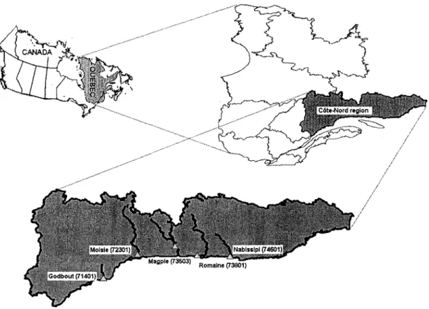
Figure 3 : Location map of the five studied rivers in the province of Quebec,

Canada ... 35

Figure 4 : Comparison of the methodologies of Asselin et al. [2005] and Perreault

et al. [2000a,2000b] on a single shift detection in a bivariate data set

(flood peaks data at stations 73301 and 73801): a) discharge; b)

Perreault et al. [2000a]; c) Asselin et al. [2005] ... 36

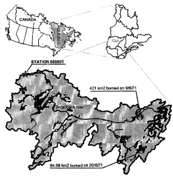
Figure 5 : Location map of station 080801 ... 37

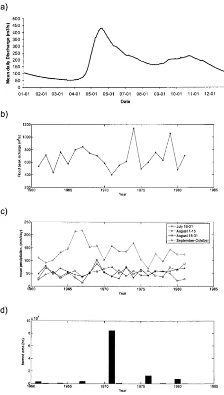
Figure 6 : Data for changepoint detection in summer-autumn flood peaks of the

Broadback river: a) mean hydrograph; b) flood peaks time series; c) precipitation time series; d) burned area time series ... 38

Figure 7 : Changepoint detection in summer-autumn flood peaks of the Broadback

river: a) posterior probability of changepoint obtained with the

methodology of Rasmussen [2001]; b) posterior probability of

changepoint obtained with the methodology of Asselin et al. [2005] ... 39

Figure 8 : Posterior probability distributions of the coefficients of the linear

regression describing the relationship between Summer-Autumn flood peaks and precipitations on the Broadback River's basin ... .40

Figure 9 : Root mean square error of model [5] for a given position of the date of

change ... 41

Figure 10 : Changepoint detection on the five rivers of Northern Quebec: a) flood

peak time series; b) posterior probability of changepoint. ... 42

Figure 11: Estimations and credible intervals for missing data: a) station 74601;

Table 1 : Table 2: Table 3:

LISTE OF TABLES

Characteristics of the five rivers of Northern Quebec ... 31 Basin scale precipitation and summer-autumn flood peaks time series for the Broadback river basin ... 31 Mean value and credibility intervals before and after the changepoint for the coefficients of the linear regression describing the relationship between Summer-Autumn flood peaks and precipitations on the Broadback River's basin ... 32

1 INTRODUCTION

Prior to the nineties, stationarity was a common assumption in statistical analyses of hydrological time series. This assumption seems less and less reasonable as a growing number of studies reveal evidence of changes in hydrological time series, presumably caused by global warming [e.g. Salinger, 2005; Woo et Thome, 2003;

Bum et Elnur, 2002]. Possible reasons of change in statistical characteristics of observed data series include natural or anthropogenic actions on the physical environment (deforestation, construction of hydraulic structures, pollution, etc.), and modifications in measurement equipment or operation protocol. Detection of eventual changes in collected data sets is obviously an important step before performing any descriptive or predictive analysis.

The authors developed in a companion Report [Ouarda et al., 2005] a general Bayesian approach to changepoint detection in multiple linear regressions that generalizes the approaches of Perreault et al. [2000a,b,c] and [Rasmussen, 2001]. It is applied here to five different examples to illustrate its features and flexibility : 1) a single shift detection in univariate data, 2) a single shift detection in multivariate data, 3) a trend change detection in univariate data, 4) a changepoint detection in univariate data with several covariates, and 5) a case of shift detection and missing data estimation in a multivariate data set. The first three examples aim to prove that the proposed methodology gives the same results that the above mentioned approaches when applied to the same data sets with the sa me prior assumptions. The two last illustrate the additional features of the proposed approach and prove

that it can be applied to cases where the other published methodologies are inadequate.

The outline of the paper is as follows : in Section 2, we present a brief summary of the changepoint models that will be used in the examples : the single changepoint detection approach in the general linear model of Rasmussen [2001], the single changepoint detection approach in the univariate normal model of Perreault et al. [2000a,b], the single changepoint detection approach in the multivariate normal model of Perreault et al. [2000a,b] and the general changepoint detection approach in a multivariate linear regression developed in the companion paper by the authors. In Section 3, the five examples are described in detail and the results of the application of the methodology to each example as weil as a brief discussion are presented. Section 4 is a general discussion about the strength of the new methodology compared to the other approaches. A conclusion is finally presented in section 5.

2 THE BAYESIAN CHANGEPOINT DETECTION MODELS

We focus here on three changepoint models that will be compared to the proposed methodology : the model of single shift detection in univariate data developed by

Perreault et al [2000a, 2000b], the model of single shift detection in multivariate normal data of Perreault et al. [2000c], and the changepoint detection model in the general linear model developed by Rasmussen [2001]. A brief summary of the model developed in the companion paper is also presented. The reader is referred to the companion paper for a more complete survey of Bayesian changepoint models.

2.1 SINGLE CHANGEPOINT DETECTION IN A NORMAL

UNIVARIATE RANDOM SAMPLE

The single shift in a normal random sample can be represented by the following model:

[1 ]

where r is the date of change, 0'2 the variance, /1! and /12 the mean before and after the change. This problem was first addressed in a Bayesian context by

Chemoff and Zacks [1963], followed by several others [Smith, 1975; Lee and

Heighinian, 1977; Booth and smith, 1982; Bruneau and Rassam, 1983; Perreault et

al., 2000a, 2000b]. The differences in the above mentioned approaches Iy mainly in the prior distributions of the unknown parameters. Perreault et al. [2000a, 2000b] derived the exact analytical expression of the posterior probability of the time and

amplitude of the shift under the assumption of constant variance. Inferences are based on the analysis of posterior distributions and are conditional upon the fact that a change happened with certainty. The following additional assumptions were made about the prior distributions:

• The prior distribution of the date of change p(r) is independent of that of

• The prior distribution of JlI is normal with parameters <1>1 and Â,0-2,

• The prior distribution of Jl₂ is normal with parameters <1>2 and ~0-2,

• The prior distribution of 0-2 is inverted gamma with parameters

a

fJ .

The posterior density of the changepoint is then :

2.2 SINGLE CHANGEPOINT DETECTION IN A MULTIVARIATE

RANDOM SAMPLE

Perreault et al. [2000c] generalized the approach presented in section 2.1 to the case of a changepoint in a multivariate sam pie. The equations are quite similar except that the parameters are now p-dimensional. The multivariate normal

distribution replaces the univariate one and the inverse Wishart distribution is used instead of the inverse Gamma distribution.

[3]

where Np stands for the multivariate normal distribution.

As in the univariate case, the following assumptions are made about the prior distributions:

• The prior distribution of the date of change peT) is independent of that of

(ft,P),

• The prior distribution of ft, is multivariate normal with parameters <1>, and

~P,

• The prior distribution of ft₂ is normal with parameters <1>2 and ~P,

• The prior distribution of P is inverse Wishart with parameters a and B.

Under these assumptions, the posterior density of the changepoint

Where ~ =~ +T,

[4]

n y.

Yn-r=

'L-' ,

2.3 SINGLE CHANGEPOINT DETECTION IN THE GENERAL

LlNEAR REGRESSION

Rasmussen [2001] considered the Bayesian estimation of changepoint in the general linear model for which the mean at a given time

i

M basis functionsgk(i), i=k, .. ,M. The basis functionsgkO are function of the observation time, and may just represent a time series of explanatory variables such as precipitation or temperature.

y~. 1 M N(Ib~gk(t),a2), t = 1, ... , r k=1 M N(Ibigk(t),a2), t=r+l, ... ,n k=1 [5]

Rasmussen [2001] takes advantage of the fact that for a given value of r, equation [5] can be written in matrix form as a plain linear regression equation :

[6]

The values of FT and 0 are equivalent to those given in Asselin et al. [2005], equation [4] and appendix 1, keeping in mind that XI

=

b1 l b 2 1 b2 l b2 2

p;

=

P;

=

Assuming a uniform distribution for the elements of 0, for logea) and for any parameter of the basis functions, the posterior distribution of the date of change is obtained:

[7]

2.4 GENERAL CHANGEPOINT DETECTION IN MULTIPLE LlNEAR

REGRESSION USING GIBBS SAMPLING.

This model was developed in the companion paper and can be represented by :

[8]

where XI is a vector of explanatory variables, {uJ are independent and identically errors following N[O,2:;y] , and

[9]

Equation [8] is rewritten using the multivariate normal distribution to be consistent with the notations of the three other methods (equations [1], [3] and [5]) :

[10]

The models presented by Perreault et al. [2000a, 2000b, 2000c] and Rasmussen [2001] can ail be represented by equation [8]. Asselin et al. [2005] considered a general prior specification for regression parameters as weil as for the variance structure, so the posterior parameter distributions could not be obtained in a closed analytical form as in the above mentioned methodologies. Gibbs sampling is thus used to obtain empirical posterior distributions for each parameter. [To test the convergence of a given parameter, the standard t-test at 95% confidence level is

used to test if the trend of that parameter is significantly different from zero.] It is assumed that the parameter has converged if the test is negative. For extensive details on prior specification and MCMC inference for model [10] we refer the reader to the companion paper [Asse/in et al. 2005].

3 APPLICATIONS

ln this section five examples in hydrology are analysed using applicable methods among those that have been described in section 2. Some of the examples were presented in previous publications. These examples are considered to allow for a rational comparison of the original methodologies with the approach proposed in this paper. These examples are:

• Example 1 : this example was drawn from Rasmussen [2001] and deals with a single shift detection in the St-Lawrence streamflows data at Ogdensbourg, New York. The analysis was performed using the methodology of Perreault et al. [2000a,2000b] (models [1]), Rasmussen [2001] (model [5]) and Asselin et al. [2005] (model [8]).

• Example 2 : the same data set as in example 1 was considered, but the data is assumed to display a linear trend followed by a constant mean. This problem was also drawn from Rasmussen [2001] and inference was performed for models [5] (Rasmussen [2001]) and [8].

• Example 3 : Models [3] and [8] were used for the detection of a single shift detection in bivariate data using the data of the Moisie and Romaine rivers located in Northern Quebec.

• Example 4 : this example deals with a single changepoint detection in the multiple linear regression between mean basin scale precipitation at four different periods of the year and the summer-autumn flood peaks of the Broadback River located in Northern Quebec, Canada. Inference was

performed for models [5] and [8].

• Example 5: the data of five rivers of the Côte-Nord region, Quebec is investigated for a single shift using model [8]. Model [3] [Perreault et al., 2000c] could not be used in this case because of several gaps in the observations.

3.1 SINGLE SHIFT DETECTION IN THE ST-LAWRENCE

STREAMFLOW DATA

We consider the 1861-1950 an nuai streamflows of the St-Lawrence River at Ogdensbourg, New York. This data set was analysed in Rasmussen [2001]. The data is plotted in Figure 1 a and seems to indicate that mean an nuai flow of that river displays either a downward trend of a negative shift. As this example is very simple, ail the models presented in section 2 can be used except that of Perreault

et al [2000c] whish is intended to work on multivariate data sets only. Models [1], [5] and [8] were thus applied to the data set.

3.1.1 PRIOR SPECIFICATION AND INFERENCES ON MODEl PARAMETERS The posterior distributions for model 3 [Rasmussen, 2001] were obtained using Jeffrey's non informative priors for the parameters. Consequently, no prior specifications are required for this particular approach. The prior distributions for the parameters of the two other models were thus set to be non informative in order to allow for a rational comparison of the various approaches. r was assumed to be uniformly distributed over

{l, ...

,n}

a

fi

distribution of mean var(Y) and infinite variance [see Perreault et al., 2000b], while

,.1, was set to 10000. For model [8], the prior mean for

e

mean, and the prior variance of

e

The posteriors distributions of models [1] and [3] where obtained using their analytical expressions (equations [2] and [7]). To make inferences on the parameters of model [8], 10000 iterations of the Gibbs sampler were performed. Convergence was successfully assessed at iteration 100. Inferences on model parameters were performed using the 9900 last iterations.

3.1.2 RESUL TS

The posterior distributions of the date of change are plotted in Figures 1 b, 1 c and 1d for models [1], [5] and [8] respectively. It appears that the three models display the sa me shape for the posterior prabability of the date of change. The mode and 95% credibility interval for ail the three models are 1891 and [1886 1894]. The results of model [1] [Perreault et al., 2000a, 2000b] and [5] [Rasmussen, 2001] are particularly similar, although there are very small differences in the posterior distributions due different model parameterisations. Model [8] gives a posterior distribution that is also very close to the two others. Note that it was not necessarily expected that empirical distributions computed fram MCMC chains would fit exactly the analytical solution. Variability due to numerical errors and the limited size of MCMC chains will always be present. The results presented in Figure 1 are thus very satisfying and can be considered as a successful validation of the praposed methodology for the case of univariate normal data with a single shift.

3.2 LlNEAR TREND FOLLOWED BV A CONSTANT MEAN IN THE

ST-LAWRENCE STREAMFLOWS DATA

This example also uses the 1861-1950 annual streamflows of the St-Lawrence River at Ogdensbourg, New York and corresponds to the second example presented in Rasmussen [2001]. It is assumed that the data set displays a linear trend followed by a constant mean, with continuity of the mean at the changepoint. Due to the presence of a trend, models [1] and [3] could not be used.

3.2.1 PRIOR SPECIFICATION AND INFERENCES ON MODEl PARAMETERS As mentioned before, priors for model [5] are always non informative. Non-informative priors are thus required for model [8] for the results to be comparable. As the methodology of Asselin at al. [2002] permits the use of informative priors, an equal weight for prior probability of the existence of a change ( r = 1, ... , n -1 ) and the absence of change (r = n) was also considered. Inferences for Model [8] were thus

performed with two different prior assumptions on the date of change: a) a uniform prior probability of the changepoint on the interval 1, ... ,n (i.e.p(r)=,Yn,r=1, ... ,n) and b) an equal weight for prior probability of the existence of a change and the absence of change (i.e.p(r)= X(n-1)' r=1, ... ,n-l and p(n) =

h)'

Inference for model [8] was performed with using 10000 iterations as in example 1 Convergence was also successfully assessed at iteration 100, and the 9900 last iterations were used to compute the posterior probability densities.

3.2.2

The posterior distributions of the two models [5] and [8] in the case of fiat prior are compared in Figure 2a. The mode and 95% credibility interval for the posterior probability distribution of the date of change obtained with model [5] are 1899 and [1893 1939] respectively. Model [8] gives approximatively the same values: 1900 for the mode and [1894 1939] for the 95% credibility intervals. It also appears that the posterior probabilities have the same shape. As mentioned earlier, it was not expected that empirical distributions computed from MCMC chains would fit exactly the analytical solution. The empirical posterior distribution of the date of change obtained from the 9900 iterations of the Gibbs sampler are fairly close to the analytical solution of [Rasmussen, 2001], and the result is considered satisfying.

Figure 2.b compares the two approaches when equal weights are given to the hypotheses of change and no change. The result is essentially the sa me as in Figure 2a except that a weight of 0.07 is obtained for the absence of changepoint

( 'r

=

'r < n are the same as in the case of fiat prior. Since the weight for 'r = n is significantly lower than the prior probability of no change, the results pleads for a strong evidence of change in the data set.

For illustration purposes, the model mean is represented in Figure 2c along with the observed streamflows, considering a changepoint at the year 1900. Visual inspection of that figure shows the excellent fit of this model for the studied data set.

3.3 SINGLE SHIFT DETECTION IN BIVARIATE

STREAM FLOW

DATA

We now compare the methodologies of Perreault et al. [2000c] (model [3]) and

Asselin et al. [2005] (model [8]) on two series of maximum flood peaks of two rivers in the Côte-Nord region of the Province of Quebec, Canada: the an nuai flood peaks of the Moisie river at station 72301, and those of the Romaine river at station 73801 for which concomitant observations are available for the period 1966-1998. The characteristic of these rivers are listed in Table 1, along with three other rivers that will be used in further examples. The location of the hydrometric stations is also given in Figure 3. The flood peak time series are presented in Figure 4a. Inspection of that Figure strongly suggests that a decrease in flows magnitude may have occurred between 1978 and 1980.

3.3.1 PRIOR SPECIFICATION AND INFERENCES ON MODEl PARAMETERS A uniform prior distribution of the date of change was considered for the two models Le. peT)

=

Yn

=

~ = a = 5 (as pointed out in Perreault et al. [2000c] , Â and a can be considered as degrees of freedom and set equal to the number of years used for prior specification), and B

=

The following values were obtained for model [8] :

v

=

=

=

and 2:0

=

variability to 9 and the other half to the random effect. Recall that the expectation of an Inverse-Wishart is E(2:)

=

0.5XCOV(Y1966_1970) for 2:y •

Inferences for the two models were performed in the same way as in the preceding examples. The burn-in period was set to 100 and inferences on model [8] parameters were performed using the 9900 last iterations.

3.3.2 RE5U L T5

Figures 4b and 4c present the results of the changepoint analysis using the two approaches. As in the two first examples, the two models gave almost exactly the posterior probability distributions. The mode and 95% credibility interval for ail the three models are 1979 and [1978 1982]. The date with the maximum posterior probability of change is 1979, which is five earlier lower than the change date of 1984 that was obtained by Perreault et al. [2000c] on a data set of six rivers in the sa me region. However, this is not a contradiction since the results are data driven

and depends on the chosen priors. Furthermore, the rivers used by Perreault et al. [2000c] are spread out in the North-Eastern part of Ouebec and in Labrador while the two sites of this example are very close to each others. The two results support the evidence of a change of streamflow regimes in northern Ouebec between 1979 and 1984.

3.4 CHANGE DETECTION IN A MUlTIVARIATE REGRESSION

MODEl : INFLUENCE OF FOREST

FI RES

ON

SUMMER-AUTUMN FLOOD PEAKS OF THE BROADBACK RIVER

The changepoint detection methods will now be applied to the relationship between summer-autumn maximum flood discharge and precipitation at station 80801 located on the Broadback River, Ouebec, Canada. This river has a catch ment of 17100 km2 and experiences from time to time fo re st fire bursts (Figure 5). According to the Canadian Large Fire Database [Stocks et al., 2002; Natural

Resources Canada, 2005], major forest fires occurred during the summer of 1971, burning 506 km2 in the upper parts of the catch ment (1/34 of the total basin area). It is hypothesized that the deforestation due to these fires has changed the basin response function to meteorological inputs. In order to perform the analysis, 1961-1981 daily flood discharges at station 80801 were obtained from Ouebec Ministry of Environment. The Broadback River is subject to two types of floods: spring flood, which are dominated by snowmelt, and summer-autumn floods which are caused by direct liquid precipitations. Figure 6a presents the mean daily discharge at this station for 1961-1981. It appears that summer-autumn maximum flood peak is generally observed at the end of October (Figure 6.a). Daily precipitations of July-October from 1961 to 1981 were obtained by interpolation from the

neighbouring weather stations on a regularly spaced grid of 100*100 points and averaged to have a time series representing precipitation at the catchments scale. This time series was then used to obtain the mean precipitation on the Broadback river catch ment for every half month from July to October. Exploratory analysis of the linear relationship between observed flood discharge and the obtained precipitation series led to the choice of four explanatory variables for the flood peak values: 1) the mean precipitations of 16-31 July, 2) the sum of precipitations of 1-15 August, 3) the sum of precipitations of 16-31 August and 4) the sum of precipitations of September-October. The values of 1961-1981 summer-autumn flood peaks are presented in Figure 6b and those of the chosen explanatory variables in Figure 6c. Figure 6d presents the burned areas on the catchment for each year of the period of study. The series of explanatory variables as weil as the maximum flood peaks are summarized in Table 2.

3.4.1 PRIOR SPECIFICATION AND INFERENCES ON MODEl PARAMETERS An equal weight was set for the probability of change (r

=

a

application ft_t

=

=

the prior mean and the prior variance for (). These consideration led to

Ô

_Ô

reg

parameters obtained using ordinary least squares, and

As for the first example, 10000 iterations of the Gibbs sampler were performed. Convergence was successfully assessed at iteration 100. Inferences on model parameter were performed using the 9900 last iterations.

3.4.2 RESUL TS

Figure 7a presents the posterior probability of the date of change obtained with the approach of Rasmussen [2001]. The maximum posterior distribution of the date of change is maximal at the beginning and at the end of the series, and displays no peak. This king of shape of posterior distribution of date of change is typical of model [5] when applied to homogeneous series. Thus the application of this approach leads to a 'no change' conclusion.

The posterior probability of the date of change obtained the approach of Asselin et

al. [2005] are given in Figure 7b. The mode and credibility interval for the posterior probability distribution of the date of change obtained with model [8] are 1972 and [1972 1978] respectively. It shows a clear peak at 1972 leading to a strong conclusion of change between 1972 and 1973. The mode and credibility intervals before and after the changepoint for each coefficient of the linear regression were computed from the MCMC chains and listed in table 3. The posterior probability distributions of these coefficients are given in Figure 8. Inspection of these distributions show that the weight of the sum of precipitations of July 16-31 decreased to negative values while that of the sums of precipitations of August

1-15 and August 16-31 increased significantly. The negative values in the regression coefficients after the changepoint can be explained by dependence between the sums of precipitations of consecutive periods. This dependence could have been removed using techniques such as principal component analysis (CCA), but such task is beyond the scope of this paper and is not supposed to change the existence and date of change in the linear relationship. The uncertainty on the regression coefficients is also higher after the changepoint since the 95% credibility interval is wider in ail cases (Table 3).

Since the two approaches give dramatically different results, an alternative procedures was sought to check whether there was a change in 1972 of not. It is simply a plot of the root mean square error (rmse) of model [5] for a given position of the date of change (Figure 9). If the rmse for a given date of change is significantly lower that the rmse at the beginning or the end of the series, it means that the model with a changepoint at that particular year give a betler fit to the data than the model with no changepoint. The plot in Figure 9 supports the hypothesis of change in 1972.

The main reason for which model [5] failed to detect the changepoint is the prior specification. It considers a noninformative prior for the regression coefficients and thus give a prior weight to physically impossible values. The prior specification for model [8] takes advantage of the fact that flood peaks are positive values and leads to the detection of a change.

3.5 SINGLE SHIFT DETECTION IN A MULTIVARIATE

DATAS ET

WITH MISSING DATA.

The two rivers presented in section 3.3 are located in the same hydrographical region of the province of Quebec and display a common date of change. Although the analysis could not explain the reason of the change, it seemed reasonable to think that the sa me cause have influenced the neighbouring rivers. As ail the other stations of the same hydrological region display a significant amount of missing data, only the approach of Asselin et al. [2005] could be used in this case. Five of these rivers were selected to have a sufficiently long common period of observation to set up the prior distributions. The selected rivers were the Godbout river (station 71401), the Moisie river (station 72301), the Magpie river (station 73503), the Romaine river (station 73801) and the saint-Paul river (station 74601), which ail have observations during the period 1975-1987. The characteristics of these rivers are listed in Table 1, and their annual maximum flood peaks are plotted in Figure 10a.

3.5.1 PRIOR SPECIFICATION AND INFERENCES ON MODEl PARAMETERS The prior specification for

e

only the common period of observation was used to compute

ê

,

:t;g

Jeffrey's non informative prior was first used for Ly (v ~ -1 and

1

sampler were performed and convergence was successfully assessed after iteration 5000.

3.5.2 RESULTS

Figure 10.b presents the posterior probability distribution of the date of change for model [8]. The posterior probability is almost entirely concentrated in 1978. This result is one year lower than that obtained in section 3.3 with only two of the rivers. It could be concluded that there is an evidence of regional change in rivers flows of the Côte-Nord region in the province of Quebec between 1978 and 1979.

The most interesting aspect of this application is the straight-forward estimation of missing data in a context of non-stationarity. As mentioned earlier, there was a significant number of gaps in the streamflow data of the Côte-Nord region. Estimation of the missing values is not an easy task even with a stationarity hypothesis. The methodology of Asselin et al [2005] addresses this issue in a straight-forward manner, and the obtained posterior distributions allow a full assessment of the uncertainty associated with the results. The reconstituted streamflows in which missing values are estimated by the mean of their posterior distributions are given in Figure 11. The credibility intervals for missing data are also provided on the same Figure.

4 DISCUSSION

The five examples presented in this paper show that the approach of Asselin et al. [2005] is very flexible and can be applied to a wide range of problems in hydrology. ln Examples 1 to 3, it is compared to published changepoint detection approaches with the sa me priors and data and it gave exactly the same results. In example 4, it is shown that it gives better results than Rasmussen [2001] on the problem of changepoint detection in summer-autumn flood peaks of the Broadback River probably because it allows for a more realistic but still vague prior specification on regression parameters as weil as on the variance parameter.

This flexibility leads to non explicit solutions for the posterior probability distributions, thus to lengthy MCMC simulations. While the approaches of

Rasmussen [2001] and Perreault [200a, 2000b, 2000c] elegantly provide posterior distributions in closed forms, and do not experience convergence problems. However, model flexibility is a requirement for a realistic analysis of hydrological data sets and the proposed methodology can be applied to a much broader range of problems : for instance, example 5 is of particular importance for hydrologists since it also allows the estimation of missing data estimation in a non-stationnary context, along with a full uncertainty assessment of the results. The posterior probability distribution of each missing data holds account of the uncertainty on the date of change, on regression parameters as weil as on the variance-covariance structure. The results are thus much more informative than any classical estimation with confidence intervals often based on unverified regularity hypotheses.

Number of other hydrological problems can be analysed with the changepoint detection methodology su ch as homogenization of historical data, hydrological neighbourhood delineation or estimation of missing data in the explicative variables. While multiple changes in rivers streamflows are relatively rare due to the sm ail length of historical series, some of these problems can easily display more than one changepoints. An interesting but quite straightforward topic of further work would be the generalisation of the approach to multiple changepoints problems. This topic was briefly discussed in Section 6 of the companion paper and should be the next step in the development of the methodology.

Another interesting development is the extension of the approach to the analysis of series of unequal variances. Such developments would broaden the range of problems that can be analysed.

5 CONCLUSION

The general approaeh to the Bayesian analysis of the multivariate regression model of Asselin et al. [2005] was eompared to reeently published ehangepoint methodologies on five seleeted examples. The results show that a) the proposed model ean handle multivariate data an/or missing values, b) it can be used with both informative and noninformative priors on the regression parameters and e) it is able to reproduee the results of Rasmussen [2001] as weil as those of Perreault

et al. [2000a, 2000b, 2000e]. Furthermore, it is shown that it ean be readily applied to hydrologie problems that are addressed by none of the above mentioned approaehes.

6 ACKNOWLEDGEMENT

The financial support provided by the Natural Sciences and Engineering Research Council of Canada (NSERC), the Northern Study Center (CEN) of Laval University and the Ouranos consortium is gratefully acknowledged. The authors are also grateful to Professor P. Rasmussen, V. Fortin and to the Quebec Ministry of the Environment for having provided the data used in the case studies.

7 REFERENCES

Asselin, J.J.J, Ouarda, T.B.M.J. and Seidou, O. (2005). Bayesian Multivariate Linear Regression with Application to Changepoint Models in Hydrometeorological Variables. Part 1. Model Development. Submitted to Water Resourees Researeh. Booth, N.B. and Smith, A.F.M. (1982). A Bayesian approach to retrospective identification of change-points. J. Econometries; 19 : 7-22.

Bruneau, P. and Rassam, J.-C. (1983). Application d'un modeïe baye'sien de delection de changements de moyennes dans une série. J. Sei. Hydro/.; 28: 341-354.

Burn, D.H. and Hag Elnur, M.A., (2002). Detection of hydrologie trends and variability. Journa/ofHydr%gy;255: 107-122.

Chernoff, H. and Zacks, S., 1963. Estimating the current mean of a normal distribution which is subjected to changes in time. Ann. Math. Statist.; 35 : 999-1028.

Lee, A.S.F. and Heghinian, S.M., 1977. A shift of the mean level in a sequence of independent normal random variables-a Bayesian approach. Teehnometries; 19 : 503-506.

Natural Resources Canada. (2005). Canadian Large Fires Database. Online

document [http://fire.cfs.nrcan.gc.ca/Downloads/LFDB/LFD_5999_e.ZIP].

downloaded on August 2005.

Perreault, L., Bernier, J., Bobée, B., and Parent, E. (2000a). Bayesian change-point analysis in hydrometeorological time series 1. Part 1. The normal model revisited. J. of Hydr%gy; 235 : 221-241 .

Perreault, L., Bernier, J., Bobée, B., and Parent, E. (2000b). Bayesian point analysis in hydrometeorological time series 2. Part 2. Comparison of change-point models and forecasting. J. of Hydr%gy; 235 : 242-263.

Perreault, L., Parent, É., Bernier, J., and Bobée, B. (2000c). Retrospective multivariate Bayesian change-point analysis : A simultaneous single change in the mean of several hydrological sequences. Stochastic Environmental Research and Risk Assessment, 14 : 243-261 .

Rasmussen, P. (2001). Bayesian estimation of change points using the general linear model. Water Resources Research; 37 :2723-2731.

Salinger, M. (2005). Climate Variability and Change: Past, Present and Future -An Overview. Climatic Change; 70 : 9-29.

Smith, AF.M., 1975. A Bayesian approach to inference about change-point in sequence of random variables. Biometrika; 62 : 407-416.

Stocks, B.J.; Mason, J.A; Todd, J.B.; Bosch, E.M.; Wotton, B.M.; Amiro, B.D.; Flannigan, M.O.;Hirsch, K.G.; Logan, K.A; Martell, D.L.and Skinner, W.R. (2002). Large forest fires in Canada, 1959-1997. Journal of Geophysical Research

(107,8149,doi :10.1029/2001 JD000484).

Woo, M. and Thorne, R. (2003). Comment on 'Detection of hydrologie trends and va ria bility' by Burn, O.H. and Hag Elnur, M.A, 2002. Journal of Hydrology 255,

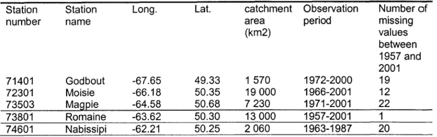
Table 1 : characteristics of the five rivers of Northern Quebec

Station Station Long. Lat. catchment Observation Number of

number na me area period missing

(km2) values between 1957 and 2001 71401 Godbout -67.65 49.33 1 570 1972-2000 19 72301 Moisie -66.18 50.35 19000 1966-2001 12 73503 Mag~ie -64.58 50.68 7230 1971-2001 22 73801 Romaine -63.62 50.30 13000 1957-2001 1 74601 Nabissi~i -62.21 50.25 2060 1963-1987 20

Table 2: Basin scale precipitation and summer-autumn flood peaks time series for the Broadback river basin.

Year Sum of Sum of Sumof Sum of

Summer-precipitations Summer-precipitations Summer-precipitations Summer-precipitations Autumn of July 16-31 of August 1- of August 16- of maximum (mm/day) 15 (mm/day) 31 (mm/day) September- flood

October peak ~mm/da~} {m3/s} 1961 47.60 24.99 29.85 110.71 535 1962 79.61 45.34 70.96 90.98 714 1963 46.52 55.41 55.76 101.69 433 1964 69.96 30.52 36.23 132.00 762 1965 56.37 49.07 53.60 146.21 572 1966 44.56 59.93 33.27 213.33 796 1967 37.91 34.25 13.84 216.20 847 1968 49.04 52.02 54.45 152.14 745 1969 102.94 88.15 57.50 157.51 702 1970 53.04 55.06 68.32 102.24 586 1971 38.67 38.29 76.19 157.44 399 1972 29.98 61.48 50.26 137.10 552 1973 75.31 39.16 71.57 135.31 612 1974 33.14 59.81 48.58 168.72 1140 1975 66.11 43.33 59.15 104.56 493 1976 42.46 41.89 60.29 69.45 603 1977 57.16 61.02 41.64 126.90 759 1978 56.95 57.92 37.51 97.12 632 1979 59.22 49.73 73.62 143.59 1060 1980 66.02 20.74 61.98 124.47 478 1981 70.38 27.73 88.40 123.76 705

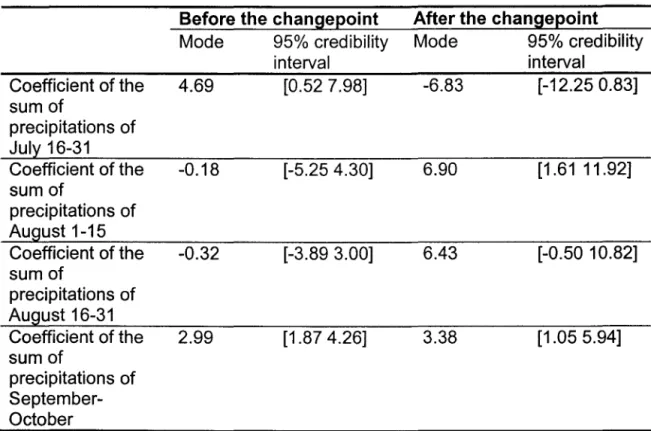
Table 3 : Mean value and credibility intervals before and after the changepoint for the coefficients of the linear regression describing the relationship between Summer-Autumn flood peaks and precipitations on the 8roadback River's basin

Coefficient of the sum of precipitations of July 16-31 Coefficient of the sum of precipitations of August 1-15 Coefficient of the sum of precipitations of August 16-31 Coefficient of the sum of precipitations of September-October

Before the changepoint Mode 95% credibility interval 4.69 [0.527.98] -0.18 [-5.25 4.30] -0.32 [-3.89 3.00] 2.99 [1.87 4.26]

After the changepoint

Mode 95% credibility interval -6.83 [-12.250.83] 6.90 [1.61 11.92] 6.43 [-0.50 10.82] 3.38 [1.05 5.94]

a) b) c) d) 300 Ji! _<.> g 260 ~ C 240 ~ E' -5 220 .!'1 0 200 180 1870 1880 1890 1900 1910 1920 1950 Year 1870 1880 1900 1910 1920 1930 Year 0.5r-~---'~~---'-~~--'--~~.--~~'---~--r~~---'~~---'-~-" '0 ~ .ll e "-·8

*

T (no change when r=1950)

1920 1930 1940 1950

1920 1930 1940 1950

Figure 1 : Comparison of the methodologies of Asselin et al [2005] , Rasmussen[2001] and Perreault [2000a] on a single shift detection in the St-Lawrence streamflow data: a) discharge; b) Perreault [2000a]; c) Rasmussen [2001]; c) Asselin et al. [2005].

a) 0.03 0.005 1870 1880 Year b) ... '0 ~ :ë cu .0 e 0.04 Cl. .g 0.03 .e '" /t 0.02 0.01 19J5O 1870 1880 1900 1910 1960 Year c) 300 - 4 -Observed flows 7ii'

't; 280 - Simulaled expecled value(changepoinl al 1900)

0 0 ~ ₂₆₀ .!S. ;= 0 240 0: c: cu ., E ₂₂₀ ëii _::l c: c: ₂₀₀ <{ 1~~60 1870 1880 1890 1900 1910 1920 1940 1950 Year

Figure 2 : Comparison of the methodologies of Asselin et al. [2005] and Rasmussen

[2001] on a trend change detection in theSt-Lawrence streamflow data: a) Posterior distributions obtained with the approaches of Rasmussen [2001] and Asselin et al.

[2005] with fiat prior on 1.; b) Posterior distributions obtained with the approaches of Rasmussen [2001] and Asselin et al. [2005] with 50%/50% prior probability of 'change'

and 'no change'; c) Discharge and simulated expected value with a changepoint at

a) 35,---,---,---,---,---,---r~====1l 10 5 1970 1975 1980 1985 1990 1995 Year b)

Histogram of the Times of Shift (methodology of Perreault[2000c])

... 0.8 'ë ~ ~ 0.6 .0 e a. 00.4 '1: J!l '" 0 a.. 0.2 0

Histogram of the Times of Shift (proposed methodology)

... 0.8 'ë ~

:g

Figure 4 : Comparison of the methodologies of Asselin et al. [2005] and Perreault et al. [2000a,2000b] on a single shift detection in a bivariate data set (flood peaks data at stations 73301 and 73801) : a) discharge; b) Perreault et al. [2000a]; c) Asselin et al. [2005].

421 km2 burned on 916n1

a) 500 ~ 450 .., §. 400 ; 350 .l!1 300 ~ 250 ~ 200 ~ 150 ." c 100 ni ~ 50 O+---_,--_,----._---r----.---~--_,----._--_,----._--._---b) c) d) 01-01 02-01 03-01 04-01 05-01 06-01 07-01 08-01 09-01 10-01 11-01 12-01 Date 1 2 0 0 , - - - , _ - - - , - - - , - - - _ , - - - , ~ 1000 "k

.

1

1

•

•

Figure 6 : Data for changepoint detection in summer-autumn flood peaks of the

Broadback river: a) mean hydrograph; b) flood peaks time series; c) precipitation time series; d) burned area time series.

a) o. ~ '0 0.15 ~ :0 tU .0 0.1 2 c. 0 'C: .$ :g 0.05 (l. 0 1962 1964 1966 1968 1970 1972 1974 1976 1978 1980 Year b) 0.7 0.6

..

Figure 7 : Changepoint detection in summer-autumn flood peaks of the Broadback river: a) posterior probability of changepoint obtained with the methodology of

Rasmussen [2001]; b} posterior probability of changepoint obtained with the methodology of Asselin et al. [2005].

a) 0.121--;::::C::=:=:::==::=:::;-~-~-~-1 o .2 0.1 ~ 0.06 ~ ~ 'Iii 0.06 §.

·i

Coefficient of the sum of precipitations of July 1&-31

Coefficient of the sum of precipitations of August 16-31

b) 0.11r======::::::;--~:-~---r-1 0.09 O.OB ~ 0.07 ~ 0.06 ~ .~ ~ 0.05 t 0.04 .~ ~ 0.03 a. 0.02 0.01 ~L5----_1~0~~--~~L----L~~~--~~--~20

Coefficient of the sum of precipitations of August 1-15 d)

0.11~-'-~-~----:1\r-==:=======ïl

- - Before the change point 0.09 O.OB ~ 0.07 ~ 0.06 ~ ~ 0.05

i

Coefficient of the sum of precipitations of Seplember-October

Figure 8 : Posterior probability distributions of the coefficients of the linear regression describing the relationship between Summer-Autumn flood peaks and precipitations on the Broadback River's basin.

160 15 150 145 140 .!!!. M

.s

Figure 9 : Root mean square error of model [5] for a given position of the date of change.

a) 4000 3500 3000 2500 ~ .!!!

..

'*

~P,;-At'l'y/H~

1.1_.

T (no change when ",2001)

1990 1990 --71401 ~72301 Ft-73503 --,)- 73801 6-74601 1995 2000 1995 2000

Figure 10 : Changepoint detection on the five rivers of Northern Quebec : a) flood peak time series; b) posterior probability of changepoint.

a) 600 550 500 { 450

f400

{

l

--+-Estimation of missing data

-Observed discharge

--.... - 95% credible Interval

1990 1995 2000

---+-Estimation of missing data

--+-Observed discharge - -- - 95% credible Interval 1990 1995 2000 b) Station 73801 2 5 0 0 , - - , - - - - , - - - , - - - . - - - - , - : - - - , - - - r = = = = = = = = ' " 2000

1

--+-Estimation of missing data

3500 - Observed discharge 95% credible Interval { 3000

j

Figure 11 : Estimations and credible intervals for missing data a) station 74601; b) station 73801; c) station 73503; d) station 72301; e) station 71401.