HAL Id: hal-01369822
https://hal.archives-ouvertes.fr/hal-01369822
Submitted on 21 Sep 2016
HAL is a multi-disciplinary open access
archive for the deposit and dissemination of sci-entific research documents, whether they are pub-lished or not. The documents may come from
L’archive ouverte pluridisciplinaire HAL, est destinée au dépôt et à la diffusion de documents scientifiques de niveau recherche, publiés ou non, émanant des établissements d’enseignement et de
Structural knowledge learning from maps for supervised
land cover/use classification: Application to the
monitoring of land cover/use maps in French Guiana
Meriam Bayoudh, Emmanuel Roux, Gilles Richard, Richard Nock
To cite this version:
Meriam Bayoudh, Emmanuel Roux, Gilles Richard, Richard Nock. Structural knowledge learn-ing from maps for supervised land cover/use classification: Application to the monitoring of land cover/use maps in French Guiana. Computers & Geosciences, Elsevier, 2015, 76, pp.31-40. �10.1016/j.cageo.2014.08.013�. �hal-01369822�
Structural knowledge learning from maps for
supervised land cover/use classification: Application
to the monitoring of land cover/use maps in French
Guiana
Meriam Bayoudha,c,∗, Emmanuel Rouxa, Gilles Richardb, Richard Nockc,d
a
ESPACE-DEV, UMR228 IRD/UMII/UR/UAG, Institut de Recherche pour le Développement
b
Institut de Recherche en Informatique de Toulouse (IRIT), UMR5505 CNRS/INPT/UPS/UT1/UTM, Toulouse, France
c
Université des Antilles et de la Guyane, France
d
Centre d’Etude et de Recherche en Economie, Gestion, Modélisation et Informatique Appliquée (CEREGMIA), Martinique, France
Abstract
The number of satellites and sensors devoted to earth observation has
be-1
come increasingly elevated, delivering extensive data, especially images. At
2
the same time, the access to such data and the tools needed to process
3
them has considerably improved. In the presence of such data flow, we need
4
automatic image interpretation methods, especially when it comes to the
5
monitoring and prediction of environmental and societal changes in highly
6
dynamic socio-environmental contexts. This could be accomplished via
arti-7
ficial intelligence.
8
∗Corresponding author. Maison de la Télédétection, 500 rue Jean-François Breton,
34093 Montpellier Cedex 5, France. Tel: +33 (0)4 67 91 72 60 Email addresses: meriam.bayoudh@ird.fr (Meriam Bayoudh ),
emmanuel.roux@ird.fr(Emmanuel Roux), richard@irit.fr (Gilles Richard), Richard.Nock@martinique.univ-ag.fr(Richard Nock)
*Manuscript
The concept described here relies on the induction of classification rules that
9
explicitly take into account structural knowledge, using Aleph, an
Induc-10
tive Logic Programming (ILP) system, combined with a multi-class
clas-11
sification procedure. This methodology was used to monitor changes in
12
land cover/use of the French Guiana coastline. One hundred and fifty-eight
13
classification rules were induced from 3 diachronic land cover/use maps
in-14
cluding 38 classes. These rules were expressed in first order logic language,
15
which makes them easily understandable by non-experts. A ten-fold
cross-16
validation gave significant average values of 84.62%, 99.57% and 77.22% for
17
classification accuracy, specificity and sensitivity, respectively. Our
method-18
ology could be beneficial to automatically classify new objects and to
facili-19
tate object-based classification procedures.
20
Keywords: Supervised classification, Machine learning, Inductive Logic Programming (ILP), Geographic Information System, Land cover map.
1. Introduction
21
The availability of remotely sensed Earth observation data, taken from
22
aircrafts (including drones) and satellites, is constantly increasing. This
ob-23
viously comes from the increasing number of Earth observation satellites
24
and sensors. In fact, a recent report (Zaiche and Smith, 2011) estimates
25
that the number of satellite launches will be 50% higher during the next
26
ten years, when compared to the last decade. In particular, 200
govern-27
mental Earth observation satellites will be launched during that period. At
28
the same time, as an increasing number of countries and/or organizations
29
distribute remotely sensed data for free, the evolution in data distribution
and use policies contributes to the use of huge volumes of data. Thus, data
31
processing and interpretation have become a serious challenge for engineers
32
and researchers. Therefore, classical procedures cannot continue to be used,
33
and new approaches are needed to automatically update the land cover/use
34
maps that provide essential information to decision makers.
35
In this context, several studies have formally represented and introduced
ex-36
pert knowledge for automatic image classification and interpretation. For
37
instance, Suzuki et al. (2001) built a system for satellite image classification
38
based on expert knowledge. More recently, Forestier et al. (2012) built a
39
knowledge-base of urban objects, allowing the interpretation of high spatial
40
resolution images in order to assist urban planner with mapping tasks.
Re-41
cent studies devoted to expert knowledge formalization for automatic image
42
interpretation have been directed towards ontologies. Hudelot et al. (2008)
43
proposed an ontology of spatial relations to guide medical image
interpre-44
tation, which is then enriched by fuzzy representations of concepts. Within
45
the remote sensing framework, both Durand et al. (2007) and Andres et al.
46
(2012) propose ontology-based automatic procedures for image processing.
47
A complementary approach to expert knowledge formalization is knowledge
48
extraction from data. Such approach is utilized by all existing supervised
49
image classification procedures, which first require a learning phase with
de-50
limitation and labeling (allocation to a class) of regions in the image.
How-51
ever, most methods consider only pixel information within such regions to
52
separate and characterize the different classes. Structural aspects, i.e.,
infor-53
mation arrangement in space, are essentially taken into account by computing
54
textural indexes within the same regions. To our knowledge, there is no
erative tool that provides general and efficient classification rules exploiting
56
structural knowledge at a higher semantic level, particularly at the object
57
level within the object-oriented image analysis (Blaschke, 2010), when such
58
knowledge is more robust and expressive than at the pixel level.
59
Automatically learning such structural knowledge within the supervised
frame-60
work, however, requires the delimitation and labeling of many more regions
61
than with pixel-based approaches, and would consequently entails important
62
expert efforts. One solution would be to take advantage of existing maps
63
resulting from different types of expertise already acquired (e.g., expertise in
64
remote sensing, image processing, environment, ecology, etc.).
65
Thus far, very few studies have proposed to learn structural knowledge from
66
maps.
67
Malerba et al. (2003) implemented INductive GEographic iNformation
Sys-68
tem (INGENS) to assist with topographic map interpretation. INGENS
con-69
sists of a prototypical extended Geographic Information System (GIS) with
70
inductive learning capabilities. GIS classical functionalities are used to
ex-71
tract relevant concepts and features from spatial database, and the integrated
72
inductive system allows finding rules to automatically recognize complex
ge-73
ographical contexts that are defined by the presence of specific geographical
74
objects and their spatial arrangement in predefined spatial windows (cells).
75
It is devoted to support map interpretation and geographical information
re-76
trieval by enriching geographical queries, but not to automatic classification
77
in the context of large datasets. In fact, such automatic procedures require
78
a quantitative evaluation that has not been performed with INGENS.
79
Vaz et al. (2007) use an Inductive Logic system called APRIL (Fonseca et al.,
2006) to learn classification rules from both a detailed map provided by
81
botanists and CORINE Land Cover (CLC) maps of the same zone. Such
82
rules are intended to automatically disaggregate CLC map information that
83
is considered too generic within the application framework. Here again, the
84
precision of the system is not provided.
85
Inductive learning of structural features from maps has been applied to the
86
prediction of particular events that partially depend on landscape
charac-87
teristics. Vaz et al. (2010) propose a system that predicts wildfires from
88
information on past fires and from compositional and structural features of
89
the land use. However, the performance of the predictions, estimated by a
90
10-fold cross validation, does not seem to allow operational use.
91
Finally, Chelghoum et al. (2006) automatically transformed spatial relation
92
information stored in multi-tables into first-order logic, and used S-TILDE
93
(Spatial Top-down Induction Logical DEcision tree) to induce classification
94
rules. They applied their method for spatial prediction of shellfish
contamina-95
tion in the Thau lagoon. Their work considered only the binary classification
96
problem.
97
In such applicative and scientific contexts, we report here a method for
98
structural and symbolic knowledge extraction from land use/cover maps and
99
complementary geographic information layers, combined with a multi-class
100
classification approach. Our work does not deal with the delimitation of
re-101
gions (or segments) from images, but with the labeling of previously defined
102
image regions. Methods intended to image region delimitation, including
103
segmentation methods, are therefore beyond the scope of this study. In this
104
study we chose the Inductive Logic Programming framework (ILP)
gleton, 1991) for the learning task, and a multi-class classification procedure
106
developed by Abudawood and Flach (2011) within the ILP framework, i.e.,
107
the Multi-class Rule Set Intersection (MRSI). This methodology was tested
108
to update land cover/use maps of the French Guiana coastline, and the
re-109
sulting classification system was thoroughly evaluated from qualitative and
110
quantitative points of view through a ten-fold cross-validation.
111
Our paper is organized as follows: the general methodology is explained,
112
by presenting the ILP approach, the geographic information extraction and
113
coding, the multi-class classification technique and the evaluation procedures.
114
Then, the application to land/use maps updating is described, by detailing
115
the exploited dataset and the adaptation of the general methodology. The
116
next section presents the results by qualifying the induced rules and
provid-117
ing prediction quantitative scores. We then discuss our results and a general
118
conclusion is given about the proposed approach.
119
2. Materials and Methods
120
2.1. Inductive Logic Programming
121
Inductive Logic Programming (ILP) (Muggleton, 1991) is a search field
122
that combines machine learning and logic programming. It is a technique for
123
learning a general theory H from a background knowledge B and examples
124
E within a framework provided by clausal logic.
125
ILP can model complex problems and has been used in several fields such
126
as chemistry (Blockeel et al., 2004), biology, physics, medicine (Luu et al.,
127
2012; Fromont et al., 2005), ecology and bio-informatics (Santos et al., 2012;
128
Lavrac and Dzeroski, 1994; Srinivasan et al., 1996). It has, also, been applied
to chess (Goodacre, 1996) and to test the quality of river water (Cordier,
130
2005). Very few studies have applied this method to geographical data, as
131
already discussed in the introduction (Malerba et al., 2003; Vaz et al., 2007,
132
2010; Chelghoum et al., 2006).
133
ILP is defined as follows (Lavrac and Dzeroski, 1994):
134
Given:
135
• A description language L.
136
• Background knowledge B, expressed under Horn clauses (a subset of
137
general first order logic formula, expressed using L, describing the
ex-138
isting knowledge and constraints on the target concept, i.e., in our case,
139
the allocation to a given land cover/use class;
140
• A set of examples E, divided into two subsets, E+ and E−, which
141
represent the sets of positive and negative examples, respectively;
142
Find a "theory" H, i.e., a set of formula using the description language
143
L that covers positive examples E+, but does not cover (or in a controlled
144
way) the negative examples E−.
145
We chose the ILP engine Aleph (Srinivasan, 2007). It is an open source
146
ILP system, written in Prolog, using top-down search and based on inverse
147
entailment (Muggleton, 1995).
148
2.2. Geographic information extraction and coding
149
Each patch of land use/cover map is referred to as object and defines
150
the elementary geographical entity to which the reasoning will be applied.
151
Objects are used to define the examples for the learning and test phases.
Objects are described using predicates characterizing their intrinsic (class,
153
area, fractal dimension, compactness, perimeter) and relational features
(ad-154
jacency, inclusion, relative positions in latitudinal and longitudinal
direc-155
tions) (cf. Table 1). The choice of such predicates is essentially based on a
156
priori knowledge of the authors on the discriminating features of the spatial
157
objects constituting land cover/use maps.
158
Inductive Logic Programming being adapted to symbolic information,
dis-159
cretization of the numeric variables is performed, and the information recoded
160
as follows: for any numeric variable V , the 10th, 20th, ..., 90th percentiles of
161
the empirical distribution of V , denoted pk(k ∈ [1, 9]), are computed. Then,
162
for every pk, two predicates were defined to indicate if an observed value X
163
for V is lower or higher than pk. For instance, the observed numeric value
164
X, corresponding to the area of the object O, is recoded, for pk, as follows:
165
area_symb(O, Ik):- area_num(O, X), X ≤ pk. or area_symb(O, Sk):- area_num(O, X), X > pk. with Ik and Sk as the intervals [− inf, pk] and ]pk, + inf], respectively.
166
Eventually, the latitude and longitude values were used to characterize the
167
relative positions of the object pairs (cf. Table 1).
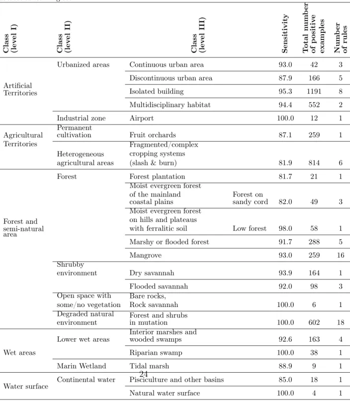
Table 1: Predicates used for object characterization. Asterisk indicates that the predicate is not used in the rule premises.
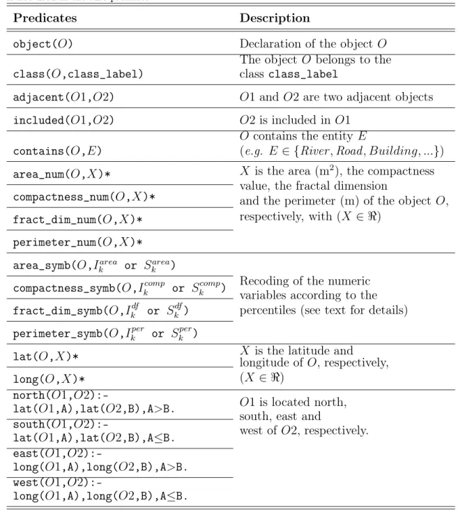
Predicates Description
object(O) Declaration of the object O
class(O,class_label)
The object O belongs to the class class_label
adjacent(O1,O2) O1 and O2 are two adjacent objects included(O1,O2) O2 is included in O1
contains(O,E)
O contains the entity E
(e.g. E ∈ {River, Road, Building, ...}) area_num(O,X)* X is the area (m2), the compactness
value, the fractal dimension
and the perimeter (m) of the object O, respectively, with (X ∈ ℜ) compactness_num(O,X)* fract_dim_num(O,X)* perimeter_num(O,X)* area_symb(O,Iarea k or Skarea)
Recoding of the numeric variables according to the percentiles (see text for details) compactness_symb(O,Ikcomp or Skcomp)
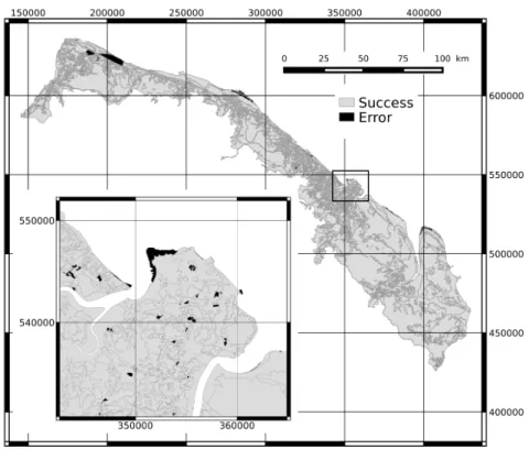
fract_dim_symb(O,Ikdf or Skdf) perimeter_symb(O,Ikper or Skper)
lat(O,X)* X is the latitude andlongitude of O, respectively, (X ∈ ℜ)
long(O,X)*
north(O1,O2):-lat(O1,A),lat(O2,B),A>B. O1 is located north, south, east and
west of O2, respectively. south(O1,O2):-lat(O1,A),lat(O2,B),A≤B. east(O1,O2):-long(O1,A),long(O2,B),A>B. west(O1,O2):-long(O1,A),long(O2,B),A≤B.
2.3. Rule induction: one-vs-rest approach
169
Once the information is extracted and coded according to the above
170
method, the classification rules are induced by the inductive system Aleph.
171
When applying ILP within the multi-class framework, i.e., in the case of more
172
than two classes (each object belonging to only one class), the one-vs-rest
173
approach is a commonly used approach (Abudawood and Flach, 2011). Such
174
method consists in generating as many classifiers as classes, by defining the
175
positive and negative example sets for each class c as follows:
176 E+= {O/classe(O, c)} E−= {O/classe(O, c)}
and by running Aleph with such example sets, for each class c.
177
2.4. Multi-class framework
178
Considering the previously described one-vs-rest approach results in
in-179
ducing as many classifiers as classes. Considering the classifiers
indepen-180
dently of one another, one or several classes can be predicted when a new
181
object is to be classified. Abudawood and Flach (2011) proposed several
182
solutions to handle multi-class problems for ILP. Among them, the
Multi-183
class Rule Set Intersection (MRSI) method gave the highest accuracies and
184
Areas Under the ROC Curve (AUC) when taking multi-class data sets into
185
account (Abudawood and Flach, 2011). The principle of the MRSI method
186
is: i) the theories induced for each class are gathered in an unique rule set;
187
ii) for each rule i, the set of covered examples by the rule, Ci, is stored; iii) a
188
default rule is formed that concludes to the majority class of the uncovered
189
examples; iv) for an unseen object O, the intersection of the sets of examples
covered by the fired rules is computed (I = ∩Ci|ri is f ired) and, finally; v)
191
the predicted class ˆc is the majority class in the set I, i.e., the more probable
192
class given to the new object O, with an empirical probability p(c|O).
193
2.5. Prediction evaluation
194
Overall accuracy, sensitivity, specificity and Kappa index are computed
195
based on a 10-fold stratified cross-validation procedure.
196
For each class Ci (i ∈ [1, n]), the set of positive examples Ei is randomly
197
divided in ten subsets Ei,f (f ∈ [1, 10]). If a class j is associated with p
198
positive examples, with p < 10, then Ei,f >p = ∅. Then the fth learning set
199
for the ith class is defined as follows:
200
Ei,f+ = ∪l=1,...,10; l6=fEi,l
Ei,f− = ∪j=1,...,n; j6=i{∪l=1,...,10 l6=fEj,l}
In the multi-class classification framework, one test set Tf has to be
de-201
fined for each fold f . Such test set is consequently defined as follows:
202
Tf = ∪i=1,...,nEi,f
Overall accuracy, sensitivity, specificity and Kappa index values are
com-203
puted for each test set, then averaged. The formulas of these measures are
204
given hereafter.
205
The multi-class classification procedure previously described permits to
com-206
pute the multi-class contingency table (see Table 2) for each test set, and to
207
obtain the overall accuracy as follows (Abudawood and Flach, 2011):
208 Overall Accuracy = n X i=1 T P(i) E (1)
where n is the number of classes, T P(i) the number of true positives for
209
the class i, and E the total number of test examples.
210
Table 2: Contingency table with notations (TP: True Positive; TN: True Negative; FP: False Positive; FN: False Negative) for the class i only. (Adapted from Abudawood and Flach (2011))
Predicted
C1 ... Ci−1 Ci Ci+1 ... Cn Total
Actual
C1 T N1(i) ... ... F P1(i) ... ... ... E1 ... ... ... ... ... ... ... ... ... ... ... ... T Ni−1(i) F Pi−1(i) ... ... ... Ei−1 Ci F N1(i) ... F Ni−1(i) T P(i) F N(i)
i+1 ... F N (i) n Ei ... ... ... ... F Pi+1(i) T Ni+1(i) ... ... Ei+1 ... ... ... ... ... ... ... ... ... Cn ... ... ... F Pn(i) ... ... T Nn(i) En Total E1ˆ ... Ei−1ˆ Eiˆ Ei+1ˆ ... Enˆ E
For each class i, the sensitivity, i.e. the ability of the classifier to
success-211
fully classified positive examples, is computed as:
212 Sensitivity(i) = T P (i) T P(i)+Pn j=1,j6=iF N (i) j = T P (i) Ei (2)
where F Nj(i) is the number of false negatives for the class i wrongly
as-213
sociated to the class j.
214
The specificity, i.e. the ability of the classifier to successfully classified
215
negative examples, is computed as:
Specif icity(i)= Pn j=1,j6=iT N (i) j Pn j=1,j6=iT N (i) j + Pn j=1,j6=iF P (i) j (3)
where T Nj(i) is the number of true negatives for the class i successfully
217
attributed to the class j and F Pj(i) the number of false positives for the class
218
i that actually belong to the class j.
219
220
Finally, the Kappa index is computed for each test set. Cohen’s Kappa
221
(Cohen, 1960) provides a statistical measure of inter-agreement for
quali-222
tative items. In the framework of classification, it measures the degree of
223
agreement between predicted and actual classes. Kappa index is defined as
224
follows:
225
kappa = P (A) − P (H)
1 − P (H) (4)
With P (A) corresponding to the observed proportion of agreement
be-226
tween two classifications, and P (H) the estimated proportion of agreement
227
expected by chance.
228
3. Application to the update of the land cover/use maps of the
229
French Guiana coastline
230
The concepts and methods previously defined were applied to an actual
231
geographic situation. The French Guiana territory is subject to intense
an-232
thropogenic and natural dynamics (Anthony et al., 2010): cyclic coastal
233
erosion and accretion, notably due to the transport of sediments from the
234
Amazon River by oceanic currents; and expansion of urban, peri-urban,
cultural areas. In this context, it is essential to develop automated methods
236
for monitoring the land cover/use of the French Guiana territory. In
partic-237
ular, the large amount of available aerial photographs and satellite images is
238
a critical source of materials that should be better exploited. If the
delim-239
itation of the geographical objects of interest does not require a high level
240
of expertise and can be performed by operators, allocating these objects to
241
land cover/use classes appears far more complex and subjective. In fact,
de-242
spite efforts made to formalize and standardize the classification procedures,
243
such allocating task requires a deep knowledge of the different types of land
244
cover/use, both in the imaging and applicative domains. Consequently, the
245
learning and classification methods previously presented were applied to
au-246
tomatically perform the labeling task and update the land cover/use maps
247
of the French Guiana coastline.
248
3.1. Dataset
249
We took advantage of a series of three land cover/use maps of the French
250
Guiana coastline for 2001, 2005 and 2008. The classification nomenclature is
251
based on the CORINE Land Cover (CLC) European nomenclature, which is
252
adapted to the Amazonian context by the addition of 15 classes, 9 of them
253
corresponding to different types of forests, and consists of three nested levels
254
where the most detailed (level III) is composed of 39 classes.
255
The maps were produced by the French National Office of Forests
(Of-256
fice National des Forêts; ONF) by photo-interpretation of the BD-Ortho R
257
aerial photographs of the French National Geographic Institute (Institut
Géo-258
graphique National: IGN) for 2001 and 2005. Air photographs had a 50-cm
259
spatial resolution. The land cover/use map for 2008 was updated using
meter spatial resolution satellite images acquired by the SPOT 5 satellite
261
and obtained through the SEAS-Guyane 1 project.
262
Figure 1: Land cover/use map and complementary geographic information layers (inset) used in this article (geographic coordinate system: WGS84 / UTM zone 22N). Sources: French National Office of Forests (Office National des Forêts; ONF); French National Geographic Institute (Institut Géographique National: IGN); French Ministry in charge of the environment; Regional Direction of the Environment (DIREN) of French Guiana ; French National Agency for Water and Aquatic Environments (ONEMA). See text for
Two complementary geographic information layers were used (see Figure
263
1): the road network, provided by the BD-Carto database of the IGN, andR
264
the river network provided by the BD-Carthage database of the FrenchR
265
Ministry in charge of the Environment and of the IGN, produced in 2009
266
for French Guiana by the Regional Direction of the Environment (DIREN)
267
of French Guiana and the French National Agency for Water and Aquatic
268
Environments (ONEMA).
269
3.2. Data pre-processing: definition of the map objects
270
Firstly, we completed the initial land cover/use classification by adding
271
three more classes: Ocean, River and Unknown. The first two classes
con-272
tribute significantly to the structure of the environment in the French Guiana
273
territory, and the Unknown class explicitly takes into account the fact that
274
information was not available for some areas in 2001 and/or 2005. However,
275
we did not induce any rules to predict membership to these three classes.
276
Finally, the class Paddy field was not considered as it was under-represented
277
in the maps (only 2 positive examples). Thus 38 land cover/use classes were
278
considered (see Tables 3, 4 and 5 for the class list).
279
In this study, we follow the land cover/use class of the objects in time. We do
280
not explicitly follow the object delimitations, which is a much more complex
281
task. In fact, by taking into account the information provided by three
orig-282
inal maps, object boundaries can change in time: an object can be splitted
283
into two or more objects belonging to different classes (see for instance object
284
s13 in figure 2), creating new object(s); an object can result from the
merg-285
ing of several objects, making one or several objects disappear. We handled
286
such situations by generating objects with invariant boundaries in time and
related to an unique class for each year. Practically, we produced a synthetic
288
map by concatenating the information contained in the three original maps,
289
by means of the "union" GIS operator, as schematically shown in Figure 2.
290
The elementary geographical entities of the resulting map are referred to as
291
objects thereafter, and contribute to define the examples in the ILP process.
292 2001 2005 2008 Synthetic map Union s11 s12 s13 s21 s22 s23 s24 s31 s32 s33 s34 s1 s2 s3 s4 s5
Synthetic map attribute table
Object (2001)Class (2005)Class (2008)Class
s1 blue blue brown
s2 brown light green light green s3 orange dark green dark green
s4 orange orange orange
s5 orange orange light green
Figure 2: Illustrative example explaining the definition of a synthetic map that combines the information from the three initial maps.
3.3. Information coding
293
Target predicates (i.e., concepts to be learned) were defined as the land
294
cover/use classes to which the objects of the synthetic map belonged in 2008,
295
considered as the reference year y0.
296
Given the diachronic characteristics of the data, 3 predicates were defined to
297
indicate the class of an object as a function of the time: class_y0(O,class_name),
298
class_y−3(O,class_name) and class_y−6(O,class_name), indicating the
299
land cover/use class of the object O for the years y0, y−3 and y−6,
tively, i.e, for 2008, 2005 and 2001. It is worth noting that from a relative
301
point of view, the year 2001, seven years prior 2008, is assumed to actually
302
correspond to the sixth year before the reference year y0. In fact, we can
303
assume marginal changes between 2001 and 2002. However, this assumption
304
has also a practical justification as it permits to consider the updating of the
305
land cover/use information every three years based on the maps established
306
three and six years before.
307
Given the complementary information layers used in our test, the predicate
308
contain(O,X) referred to rivers and roads (X ∈ {river, road}) (see Table
309
1).
310
All object features were extracted using the free and open source GRASS
311
Geographic Information System (GRASS Development Team, 1999-2012).
312
3.4. Rule induction: Aleph parametrization
313
In Aleph, the accuracy of the candidate clauses was set to 0.7, considered
314
as a good compromise between precision and generalization requirements.
315
Such accuracy is defined as p/(p+n), where p and n are the numbers of
pos-316
itive and negative examples, respectively, which are covered by the clause.
317
Consequently, it differs from the overall accuracy defined in section 2.5, which
318
evaluates the global prediction accuracy of the classification system, based
319
on the whole induced rule set.
320
The maximum premise length was set to 5 literals, such number of conditions
321
in a conjunction being practically considered as the limit for easy
compre-322
hension (Michalski, 1983).
4. Results
324
4.1. Set of induced rules
325
The induction process returned 158 classification rules for the 38 land
326
cover/use classes. However, the distribution among land cover/use classes is
327
not homogeneous (see Tables 3 to 5). For instance, we obtained 23 rules for
328
the class Forest of the old coastal plain whilst we had just one rule for the
329
Riparian swamp class. Rules cover from 2 to 692 positive examples while the
330
number of covered negative examples varied from 0 to 99.
331
Three examples of induced rules are shown below, with the number of positive
332
(Pos cover) and negative (Neg cover) examples covered by the rule, and the
333
total number of positive examples for the considered target predicate (Total
334
pos. ex.) in brackets.
335
(1) (Pos cover = 472; Neg cover = 88; Total pos. ex. = 552)
336
class_y0(A, Multidisciplinary habitat) :- area_symb(A, ≤165567),
337
adjacent(A, B), class_y−3(B, Multidisciplinary habitat).
338
(2) (Pos cover = 2 Neg cover = 0 Total pos. ex. = 40)
339
class_y0(A,Industrial or commercial area) :- adjacent(A, B),
340
class_y−6(B, Construction sites), area_symb(A, ≤10831).
341
(3) (Pos cover = 3 Neg cover = 0 Total pos. ex. = 166)
342
class_y0(A, Discontinuous urban area) :- class_y−6(A, Construction
343
sites), area_symb(A, ≤76202), area_symb(A, >10831).
344
Rule (1) covers 472 positive examples for a total of 552 objects actually
345
belonging to the class of interest (85.5%) and 88 negative examples. It
in-346
dicates that an object will belong to the Multidisciplinary habitat class if
its area is less than or equal to 165 567 m2 and is adjacent to an object
348
belonging to the same class three years before. Rule (2) indicates that an
349
object will belong to the Industrial or commercial area class if its area is
350
less than or equal to 10 831 m2 and is adjacent to an object belonging to
351
the class Construction sites 6 years before. Rule (3) indicates that an object
352
will belong to the Discontinuous urban area class if its area, in m2, belongs
353
to the interval ]10831, 76202] and if it belonged to the class Construction
354
sites 6 years before. By considering such rules for the characterization of the
355
territory dynamics, the first rule illustrates the extension dynamics of the
356
natural areas whereas the second and the third rules describe the extension
357
dynamics of the anthropogenic areas.
358
4.2. Prediction evaluation
359
Tables 3 to 5 report the sensitivity results for each land cover/use class in
360
the one-vs-rest framework by considering each classifier independently, and
361
correspond to sensitivity values that fall in the intervals ]0%, 50%], ]50%, 80%]
362
and ]80%, 100%], respectively. Among the 38 land cover/use classes, only 5
363
classes (13.1%) were associated with sensitivity values under 50%. Twelve
364
classes (31.6%) had sensitivity values between 50% and 80%, and 21 classes
365
(55.3%) had the highest sensitivity values (greater than 80%).
366
All classifiers were 100% specific, except for one related to the class Forest
367
and shrubs in mutation, which had a specificity of 83.1%.
Table 3: Averaged sensitivities obtained with 10-fold cross validation, for land cover/use classes associated with "low" sensitivity values (lower than 50%), total number of positive examples and number of induced rules for each class, by taking into account the whole dataset as learning set. (The nomenclature is based on the CORINE Land Cover (CLC) European Nomenclature with three nested levels. We applied our method to the most detailed level (level III). The nomenclature levels I and II are indicated for facilitate results interpretation only.)
C la ss (l e v e l I) C la ss (l e v e l II ) C la ss (l e v e l II I) S e n si ti v it y T o ta l n u m b e r o f p o si ti v e e x a m p le s N u m b e r o f ru le s Forest and semi-natural area
Open space with some/no vegetation beach, mud bank, dune 5.0 15 1 Forest Moist evergreen forest of the main-land coastal plain
Low forest on white sand 41.7 24 1 Artificial Territories Mine, garbage dump or construction sites Garbage dump 25.0 15 1 Construction sites 30.1 97 6 Agricultural Territories Heterogeneous agricultural areas Territories occupied mainly by agriculture with presence of vegetation 41.1 112 3
Table 4: Averaged sensitivities obtained with 10-fold cross validation, for land cover/use classes associated with "medium" sensitivity values (between 50% and 80%), total number of positive examples and number of induced rules for each class, by taking into account the whole dataset as learning set.
C la ss (l e v e l I) C la ss (l e v e l II ) C la ss (l e v e l II I) S e n si ti v it y T o ta l n u m b e r o f p o si ti v e e x a m p le s N u m b e r o f ru le s Artificial Territories
Industrial zone Industrial orcommercial area 65.0 40 2 Road network 56.9 84 3
Port 80.0 5 1
Mine, garbage
dump or construction sites Material extraction 63.5 137 5
Artificial green space 75.0 8 1
Agricultural Territories
Prairies Prairies 67.9 243 3
Arable land Arable land outof irrigation 70.0 12 1
Forest and semi-natural area
Degraded natural
environment Degraded forest 60.3 483 11
Forest Moist evergreen forest of the mainland coastal plain Coastal forest on rocks 70.0 14 3 Forest of the old coastal plain 79.9 543 23 Moist evergreen forest on hills and plateaus
with ferralitic soil High forest 76.4 194 10 Degraded natural
environment
Degraded marshy
Table 5: Averaged sensitivities obtained with 10-fold cross validation, for land cover/use classes associated with "high" sensitivity values (greater than 80%), total number of posi-tive examples and number of induced rules for each class, by taking into account the whole dataset as learning set.
C la ss (l e v e l I) C la ss (l e v e l II ) C la ss (l e v e l II I) S e n si ti v it y T o ta l n u m b e r o f p o si ti v e e x a m p le s N u m b e r o f ru le s Artificial Territories
Urbanized areas Continuous urban area 93.0 42 3 Discontinuous urban area 87.9 166 5 Isolated building 95.3 1191 8 Multidisciplinary habitat 94.4 552 2
Industrial zone Airport 100.0 12 1
Agricultural Territories
Permanent
cultivation Fruit orchards 87.1 259 1
Heterogeneous agricultural areas
Fragmented/complex cropping systems
(slash & burn) 81.9 814 6
Forest and semi-natural area
Forest Forest plantation 81.7 21 1
Moist evergreen forest of the mainland
coastal plains Forest onsandy cord 82.0 49 3 Moist evergreen forest
on hills and plateaus
with ferralitic soil Low forest 98.0 58 1 Marshy or flooded forest 91.7 288 5
Mangrove 93.0 259 16
Shrubby
environment Dry savannah 93.9 164 1 Flooded savannah 92.0 98 3 Open space with
some/no vegetation
Bare rocks,
Rock savannah 100.0 6 1
Degraded natural
environment Forest and shrubsin mutation 100.0 602 18
Wet areas
Lower wet areas Interior marshes andwooded swamps 92.6 163 4
Riparian swamp 100.0 38 1
Marin Wetland Tidal marsh 88.9 9 1
Table 6 summarizes the results for overall accuracy and Kappa Index.
369
Overall accuracy values varied from 82.4% to 87.3% with an average of 84.6%.
370
Kappa Index varied from 0.69 to 0.77 with an average value of 0.70.
371
Table 6: Kappa and overall accuracy values.
Test set 1 2 3 4 5 6 7 8 9 10 Kappa 0.69 0.67 0.74 0.71 0.75 0.68 0.69 0.73 0.60 0.77 0.70 (average) Overall accuracy (%) 83.0 87.3 84.3 85.0 84.3 85.1 84.1 83.1 87.2 82.4 84.6 (average)
4.3. Map of prediction errors
372
By regrouping the results for the 10 test sets, it was possible to construct
373
a prediction map for the year of interest (2008 in this case). Figure 3 is the
374
spatial representation of such prediction errors, highlighting that the errors
375
are not homogeneously distributed in space, two error clusters being present
376
at the extreme west and at the center of the territory.
Figure 3: Map of prediction errors (geographic coordinate system: WGS84 / UTM zone 22N). Map at the top represents French Guiana coastline; Map in the inset zooms in on the "Cayenne Island".
5. Discussion
378
From a qualitative point of view, induced rules are consistent with the
379
observed environmental features and dynamics of the study area. Moreover,
380
they are provided in an expressive formalism, and are easily understandable
381
and interpretable by non-experts, as they can be expressed in natural
lan-382
guage. However, some rules covered very few (2 or 3) positive examples,
383
whereas the total number of positive examples for the associated classes was
large (see rule (3) in paragraph 4.1 for example). Such rules were
conse-385
quently very specific and did not represent a significant knowledge within
386
the application domain.
387
The predicates south, north, east and west did not appear in the rules,
show-388
ing that such predicates were not pertinent for object discrimination, and
389
that characterization of the objects should make better use of expert
knowl-390
edge. In particular, domain ontologies could guide the learning process by
391
identifying the predicates and the learning constraints to use.
392
Whereas the maximum premise length was set to 5, induced rules comprised
393
at most 4 literals. For some classes, this can be explained by the fact that the
394
upper bound on the nodes to be explored when searching for an acceptable
395
clause (i.e., 5000, the default value) was reached and that Aleph stopped
396
before having scanned all the search space.
397
When considering the sensitivity values, we noticed that classes associated
398
with very high sensitivity (Table 5) underwent no or slow changes with time,
399
as the knowledge of the land cover type at one time in the past defined for
400
a large part the land cover type at present and in the future. It is the case
401
for very anthropogenic land use classes such as Airport and Isolated
build-402
ings or for very stable natural land cover types that cannot be exploited by
403
humans due to natural and/or legal constraints, such as Bare rocks, Rock
sa-404
vannah, Riparian swamp, or Natural water bodies. Instead, classes associated
405
with low sensitivity values (Table 3) seemed to correspond to continually and
406
rapidly shifting land cover/use types. It is more specifically the case for the
407
following classes: Beach, mud bank or dune, which is a class associated with
408
a highly dynamic environment (Anthony et al., 2010); Construction sites and
Territories occupied mainly by agriculture with presence of vegetation, which
410
is a complex class including traditional itinerant slash and burn activities
411
that consist in cultivating an area and then letting the natural vegetation
412
to regenerate. This seems to indicate that the information provided by the
413
land cover/use maps is insufficient in terms of anteriority and/or time
resolu-414
tion for these classes. However, prediction performances could be improved.
415
In fact, background knowledge can be enriched by adding predicates,
pos-416
sibly evaluated from complementary geographic information layers (digital
417
elevation model, soil map, etc.). As already mentioned, the choice of these
418
complementary object features can be guided by expert knowledge, notably
419
through domain ontologies. Better performances could also be obtained by
420
implementing different learning and classification strategies: in our case, a
421
priori known classes at year y0 could be exploited to learn more efficient
422
rules. These classes should be the most stable in time and the easiest to
423
identify (e.g. River, Continuous urban area, Airport, etc.). An iterative
424
learning-classification strategy could also be implemented, by: i) first
learn-425
ing and classifying classes associated with high-performance predictions (e.g.
426
Forest and shrubs in mutation, see Table 5); ii) then using the prediction
427
to enrich the background knowledge of other classes; iii) learning-classifying
428
these classes; iv) repeating the procedure until all classes are predicted.
How-429
ever, the number of strategies is such that we must rely on objective criteria
430
and/or intensive simulations to determine the most appropriate one.
431
Nevertheless, our method gave good results globally. In fact, in addition to
432
the excellent sensitivity and specificity values returned by the procedure, the
433
Kappa Index and overall accuracy values were high. According to the Kappa
interpretation table by (Landis and Koch, 1977), these values denote "strong
435
agreement" between predicted and actual classes.
436
The spatial representation of the prediction errors highlighted that the errors
437
are not homogeneously distributed in space. Except for the errors already
438
discussed and associated with highly dynamic environmental processes,
es-439
sentially distributed along the ocean (e.g., Beach, mud bank or dune), two
440
error clusters were identified at the extreme west and at the center of the
441
territory. Understanding such errors will require further investigation, but
442
they may be explained by the presence of errors in the initial maps.
Con-443
sequently, we suggest that the present work can also be a tool to guide the
444
validation of the existing maps.
445
Inductive Logic Programming is devoted to symbolic data. The management
446
of numeric information by ILP constitutes a specific research field, which is
447
beyond the scope of this paper. However, several simple solutions exist in
448
order to code the numeric data into symbolic ones. In fact, the domain of
449
values of a numeric variables can be categorized by means of crisp or fuzzy
450
modalities. We propose here to code the numeric information by means of
451
inequalities taking into account quantiles of the numeric variable empirical
452
distribution. This enables Aleph to manage numeric information in a manner
453
comparable to the Confidence-based Concept Discovery (C2D) ILP system
454
(Kavurucu et al., 2011). This solution seems to offer a good compromise
be-455
tween information loss and generalization capacity, by allowing the system to
456
automatically discover significant value intervals (see rule (3) in the Results
457
section).
458
Finally, the method proposed here does not consider the image processing
step devoted to the delimitation of the regions of the image that define the
ob-460
jects. It only considers the labeling (or classification) of the regions. This
im-461
plies: that the partitioning of the image into regions is performed beforehand,
462
by means of any methods including fully manual ones (photo-interpretation)
463
or automatic image segmentation algorithms; that the new objects, which
la-464
bels have to be predicted, have been delimited by the method that produced
465
the objects used for the learning task of the classification rules.
466
6. Conclusion
467
This article describes an approach inducing classification rules to
au-468
tomatically label regions of remote sensing images in order to design land
469
cover/use maps. Automatic extraction of structural knowledge using
Induc-470
tive Logic Programming was implemented and new examples were classified
471
to a unique class by means of the Multi-class Rule Set Intersection method.
472
The proposed methodology was then applied to update the land cover/use
473
of the French Guiana coastline and evaluated thoroughly.
474
We show that the induced rules provide knowledge on structural aspects.
475
The quantitative evaluation of our method demonstrated promising results,
476
allowing to offer automatic updating of the land cover/use information in
477
the study region and significant support to the operators in charge of such
478
updating. In particular, our approach could provide valuable assistance to
479
operators using object-based image analysis. In fact, such image analysis
ap-480
proach allows integrating high level symbolic knowledge concerning spatial
481
relations in the classification process. However, to our knowledge, it does
482
not offer any support to the operators in order to define efficient and general
rules that take into account such knowledge.
484
Our future work should include guiding the learning process by specifying
485
background knowledge through domain ontologies (related to remote sensing,
486
images, environment, etc.). In return, the induced rules would contribute to
487
enrich the ontologies.
488
Acknowledgements
489
This work has been performed within the framework of the project
CARTAM-490
SAT (CARtographie du Territoire AMazonien: des Satellites aux AcTeurs
491
- Dynamic mapping of Amazonian Territories: from Satellites to Actors)
492
which is funded by the European Regional Development Funds (FEDER) for
493
French Guiana: agreement number 30492. The work was also supported by
494
the GEOSUD EQUIPEX Project.
495
References
496
Abudawood, T., Flach, P.A., 2011. Learning multi-class theories in ilp, in:
497
Proceedings of the 20th international conference on Inductive logic
pro-498
gramming, Springer-Verlag, Berlin, Heidelberg. pp. 6–13.
499
Andres, S., Arvor, D., Pierkot, C., 2012. Towards an ontological approach
500
for classifying remote sensing images, in: Signal Image Technology and
501
Internet Based Systems (SITIS), 2012 Eighth International Conference on,
502
pp. 825–832.
503
Anthony, E.J., Gardel, A., Gratiot, N., Proisy, C., Allison, M.A., Dolique, F.,
504
Fromard, F., 2010. The amazon-influenced muddy coast of south america:
A review of mud-bank-shoreline interactions. Earth-Science Reviews 103,
506
99–121.
507
Blaschke, T., 2010. Object based image analysis for remote sensing. ISPRS
508
Journal of Photogrammetry and Remote Sensing 65, 2–16.
509
Blockeel, H., Dzeroski, S., Kompare, B., Kramer, S., Pfahringer, B., Laer,
510
W.V., 2004. Experiments in predicting biodegradability. Applied Artificial
511
Intelligence 18(2), 157–181.
512
Chelghoum, N., Zeitouni, K., Laugier, T., Fiandrino, A., Loubersac, L.,
513
2006. Fouille de donnees spatiales - approche basee sur la
programma-514
tion logique inductive, in: 6emes Journées d’Extraction et de Gestion des
515
Connaissances, Edition CEPADUES. pp. 529–540.
516
Cohen, J., 1960. A coefficient of agreement for nominal scales. Educational
517
and Psychological Measurement 20, 37–46.
518
Cordier, M.O., 2005. Sacadeau: A decision-aid system to improve
stream-519
water quality. ERCIM News 61, 37–38.
520
Durand, N., Derivaux, S., Forestier, G., Wemmert, C., Gançarski, P.,
Bous-521
said, O., Puissant, A., 2007. Ontology-based object recognition for remote
522
sensing image interpretation, in: Proceedings of the 19th IEEE
Interna-523
tional Conference on Tools with Artificial Intelligence - Volume 01, IEEE
524
Computer Society, Washington, DC, USA. pp. 472–479.
525
Fonseca, N.A., Silva, F., Camacho, R., 2006. April - an inductive logic
526
programming system, in: JELIA, pp. 481–484.
Forestier, G., Puissant, A., Wemmert, C., Gançarski, P., 2012.
Knowledge-528
based region labeling for remote sensing image interpretation. Computers,
529
Environment and Urban Systems 36, 470 – 480.
530
Fromont, E., Cordier, M.O., Quiniou, R., 2005. Extraction de connaissances
531
provenant de données multisources pour la caractérisation d’arythmies
car-532
diaques, in: Fouille de données complexes. Cepaduès. volume RNTI-E-4 of
533
Revue des Nouvelles Technologies de l’Information, pp. 25–45.
534
Goodacre, J., 1996. Inductive Learning of Chess Rules Using Progol. Oxford
535
University.
536
Hudelot, C., Atif, J., Bloch, I., 2008. Fuzzy spatial relation ontology for
537
image interpretation. Fuzzy Sets and Systems 159, 1929–1951.
538
Kavurucu, Y., Senkul, P., Toroslu, I., 2011. A comparative study on
ilp-539
based concept discovery systems. Expert Systems with Applications 38,
540
11598 – 11607.
541
Landis, J.R., Koch, G.G., 1977. The measurement of observer agreement for
542
categorical data. Biometrics 33, pp. 159–174.
543
Lavrac, N., Dzeroski, S., 1994. Inductive Logic Programming: Techniques
544
and Applications. Ellis Horwood.
545
Luu, T.D., Rusu, A., Walter, V., Linard, B., Poidevin, L., Ripp, R., Muller,
546
L.M.J., Raffelsberger, W., Wicker, N., Lecompte, O., Thompson, J.D.,
547
Poch, O., Nguyen, H., 2012. Kd4v: Comprehensible knowledge discovery
548
system for missense variant. Nucleic Acids Research 40, W71–W75.
Malerba, D., Esposito, F., Lanza, A., Lisi, F.A., Appice, A., 2003.
Em-550
powering a gis with inductive learning capabilities: the case of ingens.
551
Computers, Environment and Urban Systems 27, 265 – 281.
552
GRASS Development Team, 1999-2012. Welcome to grass gis.
553
http://grass.fbk.eu/.
554
Michalski, R.S., 1983. Machine learning: An artificial Intelligence Approach.
555
TIOGA Publishing Co.. chapter a theory and methodology of inductive
556
learning. pp. 110–161.
557
Muggleton, S., 1991. Inductive logic programming. New Generation
Com-558
puting 8, 295–318.
559
Muggleton, S., 1995. Inverse entailment and progol. New Generation
Com-560
puting 13, 245–286.
561
Santos, J., Nassif, H., Page, D., Muggleton, S., Sternberg, M., 2012.
Auto-562
mated identification of protein-ligand interaction features using inductive
563
logic programming: A hexose binding case study. BMC Bioinformatics 13,
564
162.
565
Srinivasan, A., 2007. The aleph
man-566
ual. http://www.cs.ox.ac.uk/activities/
567
machlearn/Aleph/aleph.html.
568
Srinivasan, A., Muggleton, S., Sternberg, M.J.E., King, R.D., 1996.
Theo-569
ries for mutagenicity: A study in first-order and feature-based induction.
570
Artificial Intelligence 85, 277–299.
Suzuki, H., Matsakis, P., Andrefouet, S., Desachy, J., 2001. Satellite image
572
classification using expert structural knowledge: A method based on fuzzy
573
partition computation and simulated annealing, in: IAMG 2001, pp. 251
574
– 268.
575
Vaz, D., Costa, V.S., Ferreira, M., 2010. Fire! firing inductive rules from
576
economic geography for fire risk detection, in: ILP, pp. 238–252.
577
Vaz, D., Ferreira, M., Lopes, R., 2007. Spatial-yap: a logic-based geographic
578
information system, in: Proceedings of the 23rd international conference
579
on Logic programming, Springer-Verlag, Berlin, Heidelberg. pp. 195–208.
580
Zaiche, L., Smith, A., 2011. 50% de satellites
581
en plus à lancer sur les dix prochaines années.
582
http://www.perspectives-spatiales.com/sites/perspectives-spatiales.com
583
/files/50%25 de satellites en plus sur la prochaine
584
décennie.pdf.