Science Arts & Métiers (SAM)
is an open access repository that collects the work of Arts et Métiers Institute of Technology researchers and makes it freely available over the web where possible.
This is an author-deposited version published in: https://sam.ensam.eu Handle ID: .http://hdl.handle.net/10985/10654
To cite this version :
Holanyo K. AKPAMA, Mohamed BEN BETTAIEB, Farid ABED-MERAIM - Numerical integration of rate-independent BCC single crystal plasticity models: comparative study of two classes of numerical algorithms - International Journal for Numerical Methods in Engineering p.97 - 2016
Any correspondence concerning this service should be sent to the repository Administrator : [email protected]
Numerical integration of rate-independent BCC single crystal plasticity
models: comparative study of two classes of numerical algorithms
Holanyo K. Akpama, Mohamed Ben Bettaieb*, Farid Abed-Meraim
LEM3, UMR CNRS 7239 – Arts et Métiers ParisTech, 4 rue Augustin Fresnel, 57078 Metz Cedex 3, France
DAMAS, Laboratory of Excellence on Design of Alloy Metals for low-mAss Structures, Université de Lorraine, France
*Correspondence to: Mohamed Ben Bettaieb; E-mail: [email protected]
Abstract
In an incremental formulation suitable to numerical implementation, the use of rate-independent theory of crystal plasticity essentially leads to four fundamental problems. The first is to determine the set of potentially active slip systems over a time increment. The second is to select the active slip systems among the potentially active ones. The third is to compute the slip rates (or the slip increments) for the active slip systems. And the last problem is the possible non-uniqueness of slip rates. The purpose of this paper is to propose satisfactory responses to the above-mentioned first three issues by presenting and comparing two novel numerical algorithms. The first algorithm is based on the usual return-mapping integration scheme, while the second follows the so-called ultimate scheme. The latter is shown to be more relevant and efficient than the former. These comparative performances are illustrated through various numerical simulations of the mechanical behavior of single crystals and polycrystalline aggregates subjected to monotonic and complex loadings. Although these algorithms are applied in this paper to Body-Centered-Cubic (BCC) crystal structures, they are quite general and suitable for integrating the constitutive equations for other crystal structures (e.g., FCC and HCP).
Keywords:
integration algorithm; finite strain; crystal plasticity; rate-independent framework; Schmid’s law; multisurface plasticity1. Introduction
Due to its ability to relate the inelastic behavior of crystalline materials to their microstructure, the modeling of the mechanical response of single crystals has remained an active research topic. The constitutive equations describing the single crystal behavior are now well understood and fairly well established (see, e.g., [14]). For a thorough look at various aspects of the constitutive modeling of single crystals, the reader may refer to earlier contributions (see, e.g., [59]). In the majority of constitutive models dedicated to single crystals, the inelastic deformation is assumed to arise solely from the slip on the crystallographic slip systems. Accordingly, deformation by diffusion, phase transformation, twinning and grain boundary sliding is not considered herein. Two different modeling frameworks have been proposed in the literature for the evolution of the slip rates: the rate-dependent and rate-independent approach. From a theoretical point of view, it is more appropriate to formulate the problem as rate-independent, especially at low temperature over a substantial range of strain rates, since most metals exhibit weak strain-rate dependency [10]. This rate-independent modeling approach is therefore adopted and studied in this paper. However, several difficulties are related to its numerical integration as will be explained hereafter.
Contrary to its theoretical modeling, the numerical integration of the single crystal behavior is still subject to debate and remains an active research topic, especially with the development of computational codes used to predict the mechanical response of metallic components and structures. These codes are generally based on the finite element (FE) method (e.g. [11], [12]), or some homogenization techniques (e.g. [1316]), or even a combination of the two strategies, such as the FE2 method (e.g. [1719]). In many situations, the number of degrees of freedom of the problem (or the size of structure) is rather large, which leads to a computationally burdensome task, because it requires a great deal of CPU time and memory space. For this reason, it is still of substantial scientific and technical interest to develop robust, efficient and accurate numerical schemes and algorithms to integrate the constitutive equations of the rate-independent theory of crystal plasticity. The purpose of this paper is to propose, after a comparison and an extensive discussion of the different choices, such a scheme.
The constitutive equations of the rate-independent theory of crystal plasticity are incrementally integrated over a typical time increment I[t0, t0t]. The main tedious task of the numerical
integration is to split the increment of the total deformation into an elastic and plastic part. As the plastic deformation is solely due to the slip on the crystallographic systems, the problem of the decomposition of the total strain increment is reduced to the determination of the slip rates (or the slip increments) of the different slip systems. The set of governing equations used to compute the slip rates is known to be generally strongly non-linear, and this non-linearity has two distinct sources. The first comes from the material behavior and is related to the expression of the hardening law (when hardening
is considered). Indeed, the hardening laws used in the literature generally assume a complex, non-linear evolution for the rates of the various critical shear stresses as a function of slip rates. The second source of non-linearity is geometrical and is related to the evolution of the crystal lattice rotation (within the finite strain modeling framework).
In the literature, there exists two main classes of algorithms to integrate this set of non-linear equations:
The first class, which is the most popular, includes the usual return-mapping algorithm for the integration of elastic–plastic constitutive equations, see, e.g., [11], [12], [20][22]. The idea behind this class of algorithms is borrowed from the numerical integration of single surface phenomenological plasticity models. It is based on the elastic predictor–plastic corrector scheme. In this case, an elastic trial stress is computed and the corresponding trial resolved shear stresses are determined by projecting the trial stress on the orientation tensor of the different slip systems. A system is said to be potentially active if its trial resolved shear stress is strictly superior to its initial critical shear stress (at t0). Thus, the set of potentially active slip systems is determined at
t0+t. This set is assumed to be unchanged over the entire time step [t0, t0+t]. Accordingly, the
return-mapping algorithm is not able to account for intermediate activation and deactivation of slip systems during the time increment. To compute the slip increments of the potentially active slip systems, the discrete Kuhn–Tucker loading condition, resulting from the Schmid criterion [23], is obviously used. This condition is defined for each potentially active slip system by two inequalities and an equality constraint as follows: the slip increment for each slip system is superior or equal to zero, the difference between the critical shear stress and the resolved shear stress is superior or equal to zero, and the product of these two positive quantities is equal to zero. This states that a slip system is active only if its slip increment is strictly positive and the difference between its resolved shear stress and its critical shear stress is equal to zero. Otherwise the system is inactive. Mathematically speaking, this Kuhn–Tucker condition may be considered as a non-smooth complementarity problem and its resolution requires careful attention. To determine the set of active slip systems among the potentially active ones, several search strategies have been employed in the literature. These search strategies are carried out iteratively and, at each iteration, a subset of the set of the potentially active slip systems is selected to be the set of active slip systems. The slip rate of each presumed active slip system is computed by enforcing the equality between its critical shear stress and its resolved shear stress. For the other slip systems, belonging to the set of the potentially active slip systems, their slip rates are assumed to be equal to zero. After this step, the Kuhn–Tucker condition is checked for all the potentially active slip systems. If at least one constraint of this condition is violated, then the assumed set is not an effective set of active slip systems and another set is chosen. Several techniques have been used in the literature to select the set of active slip systems for the next search iteration, such as the intuitive combinatorial strategy developed by Ben Bettaieb et al. [24]
and other less intuitive strategies, see e.g., [1113]. When material and/or geometrical non-linearities are considered in the modeling of the single crystal behavior, the computation of the slip increments for a given set of active slip systems requires the solution of a system of non-linear differential equations. To solve this system, two main integration schemes can be used. The first is explicit and is generally based on a forward Euler scheme. In this case, the critical shear stresses and the crystal lattice rotation are held fixed over the time increment and are equal to their values at t0. With this choice, the mathematical system becomes linear and can be solved
directly, e.g., [11]. However, the solution is not necessarily unique. In case of non-uniqueness of the solution, some rules are used to determine an optimal solution, such as the pseudo-inversion technique, e.g. [11], or the perturbation technique [12]. Due to its relative simplicity, the use of this explicit scheme allows reducing the CPU time required for each time increment, on the one hand, but, on the other hand, requires the use of a large number of very small strain increments to avoid numerical instabilities and inaccuracies. The second integration scheme used to compute the slip increments is implicit and is based on the backward Euler scheme. In this case, the critical shear stresses and the crystal lattice rotation are evaluated at t0+t. The resulting system
of non-linear differential equations is solved by traditional iterative methods, such as the Newton–Raphson technique [12], [21], [22] or the fixed point method [24]. Contrary to the explicit scheme, the implicit one permits the use of larger time increments in order to reduce the computation time. It must be noted that the non-uniqueness issue may also be encountered in the application of the implicit algorithm. When the rate-independent single crystal constitutive equations are formulated under the small strain assumption, namely without evolution of the crystal lattice rotation and without non-linear hardening (i.e., perfect plasticity or linear hardening), the explicit and the implicit schemes become obviously equivalent. Generally, the use of implicit return-mapping algorithms is rather time consuming. Indeed, such algorithms are based on two separate nested loops: the first loop is used to search the set of active slip systems and the second is employed to compute the slip increments of the active slip systems. Hence, this approach is quite computationally expensive; especially when the number of potentially active slip systems is much larger than the number of active slip systems and/or when complex loading paths are involved (abrupt change in the loading path, elastic unloading...). In order to decrease the CPU time and thus to have an efficient integration scheme, a novel implicit return-mapping algorithm is proposed in the current paper. It is based on the replacement of the two inequalities and equality constraint of the Kuhn–Tucker conditions by a system of equations involving the so-called Fischer–Burmeister complementarity function [25], [26]. In this latter case, the set of active slip systems and the corresponding slip increments are determined iteratively by solving this system, which only requires a single loop. This choice of semi-smooth form of Kuhn–Tucker condition, defined by the Fischer–Burmeister complementarity functions, leads to an alternative
method that is more efficient and robust for determining the active slip systems and their slip rates. Although this strategy is very popular in the field of mathematical optimization [27-29], and is also applied to some problems of solid mechanics, such as contact mechanics, it is unfortunately not sufficiently used to solve the Kuhn–Tucker condition of single crystals. In fact, only few works formulated in the small strain framework can be found in this context [21], [30]. Consequently, the development of this novel algorithm is one of the major contributions of this paper.
The second class of integration schemes may be built following the so-called ultimate algorithm initially introduced by Borja and Wren [31] and subsequently followed by [13], [24], [32], [33]. In this class, a slip system is considered to be potentially active if its resolved shear stress is equal to its critical shear stress at t0. Accordingly, the set of potentially active slip systems is
evaluated at t0 and the trial phase is no longer required. Another important difference is that, in
this case, the time increment may be divided into several sub-increments with the end of each sub-increment determined by the change in the set of potentially active slip systems (through addition or suppression of slip systems). Contrary to the return-mapping class, the ultimate algorithm provides not only the set of active slip systems at t0+t, but also their sequence of
activation and deactivation over the time increment. This choice allows then accounting for possible changes in the slip activity over [t0, t0+t]. For the determination of the set of active slip
systems, the iterative search strategies used in the return-mapping algorithms can also be applied to the ultimate algorithms. For example, Knockaert et al. [13] adopted a strategy very similar to that used in [11], [24], [33]. As will be demonstrated later, and unlike the return-mapping class of algorithms, the development of a fully implicit ultimate scheme is conceptually difficult. Only explicit ultimate algorithms have been developed in the literature, see e.g., [13], [31]. In the same way as before, the problem of non-uniqueness of the slip rates for a given set of active slip systems may also be encountered in the case of an ultimate algorithm, and it can be circumvented by using, for example, the pseudo-inversion technique as in [13], or the perturbation technique as in [24], [33]. The development of an explicit/implicit version of the ultimate algorithm class is the second major contribution of this paper. This algorithm is optimal in the determination of the active slip systems and in the computation of the corresponding slip increments.
Moreover, to the authors’ best knowledge, the comparison between the two classes of algorithms has not been attempted in the literature. Therefore, the third important objective of this paper is to compare, through several numerical simulations, the accuracy and the efficiency of the two novel algorithms (the return-mapping algorithm and the ultimate one). As will be shown in the sequel, it turns out that the ultimate algorithm is substantially more accurate and more efficient than the return-mapping one. It is also noteworthy that, in contrast to previous literature works, which have mostly dealt with the numerical integration of FCC single crystal constitutive equations, the present work specifically focuses
on BCC crystal structures. From a fundamental perspective, the difference in the numerical treatment of the two crystal structures is not significant. However, in practice, the higher number of slip systems in BCC single crystals, as compared to FCC single crystals, introduces additional difficulties, which thus leads to a more challenging problem.
The paper content is structured in the following way:
- Section 2 outlines the constitutive equations of single crystal plasticity in the framework of finite strain rate-independent theory, by adopting both Eulerian and Lagrangian formulations.
- Section 3 details the algorithmic developments both for the return-mapping and the ultimate algorithm in an incremental formulation. The derivation of a tangent modulus, consistent with the ultimate integration scheme, is given in the end of Section 3.
- The accuracy of the numerical predictions as well as the efficiency of the developed algorithms, in terms of computational cost, are discussed and compared in Section 4 on the basis of simulation results at the single crystal scale.
- The superiority of the ultimate algorithm compared to the return-mapping one, in terms of required computational time, is further highlighted in Section 5, where several numerical tests are carried out on polycrystalline aggregates.
- The consistent tangent modulus derived in Section 3.3 is validated in Section 6 through two numerical tests.
Notations, conventions and abbreviations
The derivations presented in this paper are carried out using classical conventions. Note that the assorted notations can be combined, while additional notations will be clarified as needed following related equations.
2. Constitutive equations
2.1. Decomposition of the elastic–plastic deformation
The classical treatment of finite deformation plasticity may be traced back to several earlier works, e.g., [1], [3], [6], [7]. It is based on the assumption of the existence of an infinite number of intermediate configurations, also called elastically relaxed configurations, obtained by elastic unloading to a stress free state. Here, only the main theoretical lines are recalled, except in some cases where equations that are essential to subsequent analyses are provided for completeness.
As a starting point, the total deformation gradient f is taken to be multiplicatively decomposed into an elastic part fe and a plastic part fp
e. p
ff f . (1)
The elastic part fe can itself be multiplicatively decomposed into a stretching tensor ve and a rotation tensor r
e
f v r . (2)
Rotation r defines the orientation of the coordinate system related to the intermediate configuration relative to the current one. It can be expressed in terms of the Euler angles 1 2 3 as
Vector and tensor variables are designated by bold letters and symbols. Scalar variables and parameters are referred to by thin letters and symbols.
Einstein’s convention of summation over repeated indices is adopted. The range of the free (resp. dummy) index is indicated before (resp. after) the corresponding equation.
time derivative of 1 inverse of inner product cross product
double contraction product
tensor product
T
transpose of tensor
tr ( ) trace of tensor
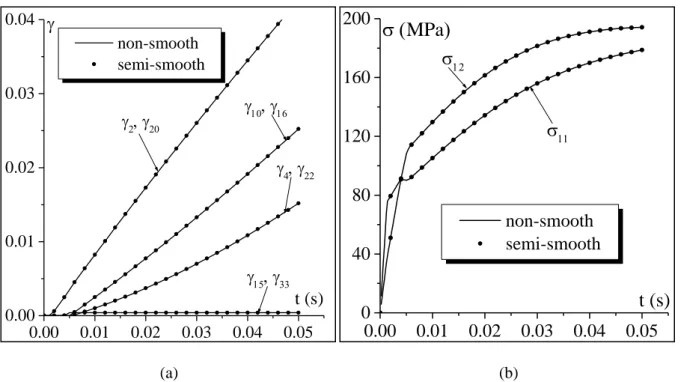
R-M and UL will be used, as needed, to specify the return-mapping and ultimate algorithm, respectively. In some figures of Sections 4, 5 and 6, for the sake of clarity and to avoid clutter, the dots associated with dotted curves are not represented for all time increments (typically only one dot is reproduced at each 5 x 10³ s).
1 2 3 1 3 2 3 1 1 3 3 2
3 1 1 2 3 1 3 2 1 3 2 3
1 2 1 2 2
cosφ cosφ cosφ sinφ sinφ cosφ cosφ sinφ cosφ sinφ cosφ sin φ cosφ sin φ cosφ cosφ sinφ cosφ cosφ cosφ sinφ sinφ sin φ sin φ
cosφ sin φ sinφ sinφ cosφ
r . (3)
The Eulerian velocity gradient g, expressed in the current configuration, is given by the following formula: 1 1 1 1 e e e p p e 1 T 1 1 T 1 e e e e e p p e . . . . . . . . . g f f f f f f f f v v v r r v v r f f r v (4)
As is the case for most metallic materials, the elastic deformation is often assumed to be very small compared to unity. Accordingly, the stretching tensor ve is very close to the second-order identity tensor
e
v 1. (5)
Combining Eqs. (4) and (5), we obtain
T 1 T
e . . p. p .
gv r r r f f r . (6)
The symmetric and anti-symmetric parts of g, denoted as d and w , respectively, are defined by
T T e p e p 1 ( ) ( ) 2 d gg d d w g g w w (7)
where the elastic and plastic parts, de and d , of the strain rate tensor p d, as well as the elastic and plastic parts, we and w , of the rotation rate tensor w are given by p
1 1 T T e e p p p p p T 1 1 T T e p p p p p 1 . . . . 2 1 . . . . . 2 d v d r f f f f r w r r w r f f f f r (8)
2.2. Discrete kinematics of single crystal
We recall that the single crystal plastic strain is assumed here to be solely due to the slip on the crystallographic slip systems. Each slip system α is defined, in the deformed configuration, by two orthogonal vectors mα and nα representing the slip direction and the normal to the slip plane, respectively. Although this paper specifically focuses on BCC single crystals, we shall assume that each crystal has in general a total of N slip systems. s N is equal to 24 for BCC crystallographic structures. s
Therefore, the integer α ranges then from 1 to N . The symmetric (resp. anti-symmetric) part of the s
tensor product Mα mα nα is denoted by Rα (resp. Sα) and is called the Schmid tensor associated with the slip system α. The rotation r between the current configuration and the intermediate one is chosen such that the tensor product mαnα of each slip system α is equal to m n0α when
expressed in the intermediate configuration. With this choice, the slip direction mα and the normal to the slip plane nα in the deformed configuration are given by the following relations (Figure 1):
0 0 1
α e . α ; α α . e
m f m n n f . (9)
Using assumption (5) and the kinematic relations (9), the tensor M , which is equal to 0α m n0α, can be related to Mα by the following relation:
0 T
α . α.
M r M r. (10)
The detailed numbering of m and0α n for BCC single crystals is given in Appendix A. 0α
As the plastic deformation is solely due to the slip on the crystallographic systems, the plastic part
1 p
. . .
r f f r of the velocity gradient (see Eq. (6)) can be written as
1 T *
p β β s
. . . γ ; β 1,...,N
r f f r M , (11)
where γ*β is the algebraic value of the slip rate of system β. For practical reasons, and for handling only
positive values of slip rates, it is more convenient to split each slip system into two opposite oriented slip systems (m , β n ) and (β mβ, n ). With this new definition, Eq. (11) becomes β
1
p β β β s
. . . γ with γ 0 ; β 1,...,2 N
r f f r M . (12)
From Eq. (12), the plastic strain rate d and plastic spin p w can be written in terms of the Schmid p
tensors R and β S as follows: β
p γβ β ; p γβ β ; β 1,...,2 Ns
d R w S . (13)
The rotation tensor r , which describes the crystallographic orientation of the single crystal and its evolution, is defined by the following relation:
T
p
.
r r w w . (14)
As in several earlier works, e.g. [24], [33], [34], Eqs. (6), (8), (11) and (13) are expressed in the crystal lattice frame defined by the rotation r in order to satisfy the objectivity principle [35]. For the sake of clarity, the tensors and vectors evaluated in this frame are denoted by an underbar notation. In this frame, the velocity gradient is expressed as follows:
T
. .
gr g r d w, (15)
where d and w are defined by the following relations:
T
e p , . p , p p γβ β ; β 1,...,2 Ns
dd d wr rw d w M . (16)
T β . β.
M r M r. (17)
By comparing Eqs. (10) and (17), we can easily conclude that the tensor product M is constant and β
equal to M0β.
2.3. Elastic behavior law
Recognizing that the deformations considered in the present paper are dominated by plastic slip, and that the elastic deformations are small in comparison to those induced by plastic slip, we consider the elasticity as being linear and isotropic in the constitutive equations for simplicity. In a rate form based on Eulerian tensors, the elastic part of the behavior law is classically written as
e: e 2μ e λ tr( )e
σ d d d 1. (18)
Here, e is the fourth-order elasticity tensor, σ is the Cauchy stress rate tensor, and λ and
μ
are the Lamé coefficients.In total form based on Lagrangian tensors, Eq. (18) can be rewritten in the following form:
e
e
, (19)
where T and e are the symmetric second Piola–Kirchhoff stress tensor relative to the intermediate e
configuration and the elastic Green–Lagrange deformation tensor, respectively, see e.g., [11]. They are defined by the following relations:
1
e e e e e
[det( )] . . ; (1/2)( )
T f f σ f e c 1 , (20)
with c being the elastic right Cauchy–Green deformation tensor given by e T
e e . e
c f f . (21)
2.4. Plastic behavior law
The plastic part of the behavior law is defined by the Schmid law [23]. This relation states that slip may occur only when the resolved shear stress τ on a slip system α becomes equal to a critical value α c
α τ c α α α s c α α α τ τ γ 0 α 1,...,2 N : τ τ γ 0 (22)
where the resolved shear stress τ , acting on a given slip system α, is defined as the projection of the α Cauchy stress on the Schmid tensor M associated with that slip system α
α α α α
and the evolution of the critical shear stress c α
τ is given by the hardening law defined in Section 2.5. By using Eqs. (9), (20)(1), (21) and (23), τ can be expressed as follows: α
, (24)
where c T is the inner product between e. c and T . e
For infinitesimal elastic stretches (det( ) 1fe and ce 1), the resolved shear stress τ can be α approximated by
0 0 0 0 0 0
α α α α α α α
τ T n. ).m T M: with M m n . (25) Considering Eq. (22), the yield function c
α (τατ )α
f corresponding to slip system α then reads c
s α α α α α α
α 1,...,2 N : (τ τ ) 0 ; γ 0 ; γ 0
f f . (26)
Eq. (26) may be viewed as a non-smooth complementarity problem and can therefore be replaced by an equivalent system involving the semi-smooth Fischer–Burmeister function [25], [26]
2
s α α α α α
α 1,...,2 N : φ ( )f (γ ) f γ 0
. (27)
2.5. Hardening description
The hardening law describes the evolution of the critical shear stress c α
τ during the loading history. The literature provides numerous models with various expressions for the hardening law, which are generally motivated by the crystal physical microstructure and are dependent, via a hardening modulus
h , on the slip rates of the different slip systems. These hardening laws have traditionally a rate form
and can be expressed as
s
c
s α+N α αβ β β+N s
α 1,..., N : τ τ h (γ γ ) ; β 1,..., N
. (28)
The hardening modulus h has been defined in the literature by various forms: diagonal, isotropic, anisotropic, symmetric or asymmetric. An overview of the different hardening laws adopted in the literature is given in [7], [36]. In the present paper, the integration scheme is general enough to be independent of the choice of the hardening law.
3. Numerical integration
We now elaborate on the algorithmic treatment of the above-described constitutive equations. In this aim, two new algorithms are developed. The first is based on the return-mapping class of algorithms, while the second relies on the so-called ultimate algorithm. For convenience, the return-mapping algorithm is formulated within a Lagrangian hyperelastic approach, whereas the ultimate algorithm is developed within an Eulerian hypoelastic framework.
0
α e α α e τ . ). . det( ) 1 c T n m fThe time integration of the constitutive equations, described by Eqs. (1)–(28), proceeds by discretizing the deformation history in time and numerically integrating these equations over each time increment I[t0, t0+t]. For this purpose, we assume that the mechanical quantities: f , e f , p σ , r , γ and α τcα (for
s
α 1,...,2 N ) are known at t0. The Eulerian velocity gradient g is assumed to be constant and known
over the time increment I. The aim of both incremental algorithms is to compute σ , r , γ and α c α τ (for α1,...,2 Ns) at t0+t. In what follows, a variable x evaluated at t0 (resp. t0+t) is denoted by
x(t0) (resp. x(t0+t)).
3.1. Return-mapping algorithm
This algorithm is defined by three main steps, which will be detailed in Sections 3.1.1, 3.1.2 and 3.1.3.
3.1.1. Determination of the set of potentially active slip systems
A direct time integration of Eq. (4) over I gives the following update equation: Δt
0 (t Δt) e g. (t )
f f . (29)
When Δt g is very small ( Δtg ), Eq. (29) can be approximated by
0
(t Δt) ( Δt ). (t )
f 1 g f . (30)
Despite the accuracy of the kinematic approximation (30) (especially for small time increments), the exact expression (29) is used in this algorithm. Note that approximation (30) is widely used in the literature (see. e.g. [11]).
The trial elastic deformation gradient tr 0 (t Δt) f is computed as tr 1 e (t0 Δt) (t0 Δt). p (t )0 f f f , (31)
in terms of which we express the trial elastic Green–Lagrange strain tensor by
tr tr tr tr T tr
e(t0 Δt) (1/2)( (te 0 Δt) ) ; e(t0 Δt) e (t0 Δt). e(t0 Δt)
e c 1 c f f . (32)
The trial second Piola–Kirchhoff stress tensor associated with the trial elastic strain tr e
e is defined by the following relation:
tr tr
0 e e 0
(t Δt) (t Δt)
T . (33)
And the trial resolved shear stresses are given by (see Eq. (25))
tr tr 0
s α 0 0 α
α 1,...,2N : τ (t Δt) T (t Δt) M
. (34)
A slip system α is potentially active if it satisfies the following inequality:
tr c
α 0 α 0
τ (t Δt) τ (t ) 0 . (35) Accordingly, the set of potentially active slip systems is given by
tr c
s α 0 α 0
α 1,...,2 N ; τ (t +Δt) τ (t ) 0
. (36)
At this stage, two possibilities may occur [37]:
If , then the mechanical behavior is purely elastic over I (i.e., there is no plastic flow) and the slip rates of all the slip systems are equal to 0. The algorithm described in Section 3.1.2 is then skipped.
If , then the mechanical behavior is elastic–plastic over I and there is at least one system that is active among the set of potentially active slip systems. To compute the slip rates of the potentially active slip systems, the algorithm detailed in Section 3.1.2 is followed.
3.1.2. Determination of the slip increments of the potentially active slip systems
Eq. (12) can be written in the frame of the crystal lattice
1
p. γβ β γβ β ; β 1,...,2Ns
f f M M . (37)
If a slip system α is not potentially active, then its slip rate γ is obviously equal to 0. Hence, Eq. (37) α can be reduced to the following form:
1 p β
. γ ; β
f f M . (38)
A backward integration of Eq. (38) yields
0
p(t0Δt) p(t ) Δγ0 β β. (tp 0Δt) ; β
f f M f , (39)
which can be written equivalently as
1
p(t ).0 p (t0 Δt) ( Δγβ ) ; β
f f 1 M . (40)
On the other hand, the elastic Green–Lagrange strain tensor can be written as
e(t0 Δt) (1/2)( (te 0 Δt) )
e c 1 . (41)
The deformation gradient f(t0Δt) can be written in the following two equivalent forms:
tr
0 e 0 p 0 e 0 p 0
(t Δt) (t Δt). (t Δt) (t Δt). (t )
f f f f f , (42)
which implies that
tr 1
e(t0 Δt) e (t0 Δt). (t ).p 0 p (t0 Δt)
f f f f . (43)
By using Eq. (43), expression (41) of the elastic Green–Lagrange strain tensor becomes
T 1 tr T tr 1 e 0 p p e e p p T 1 tr T tr 1 p p e e p p T 1 p p p p (t Δt) (1/2) (t ). (t Δt) . (t Δt). (t Δt) . (t ). (t Δt) (1/2) (t ). (t Δt) . (t Δt). (t Δt) . (t ). (t Δt) (1/2) (t ). (t Δt) . (t ). 0 0 0 0 0 0 0 0 0 0 0 0 0 0 0 e f f f f f f 1 f f f f 1 f f f f f f
(t0 Δt)
1 . (44)By substituting Eq. (40) in Eq. (44), ee(t0Δt) can be rewritten after some lengthy but straightforward algebraic manipulations as
tr tr 0 e(t0Δt) e(t0Δt) Δγ sym β e(t0Δt). β ; β e e c M , (45)where sym(x) is the symmetric part of tensor x. Note that the slip increments Δγ are assumed to be β small so that, in the expression (45) above, their second-order terms have been disregarded.
The resolved shear stress τ is determined on the basis of Eqs. (19), (25) and (45) α
0 tr tr 0 α 0 α e e 0 β e 0 β 0 tr 0 tr 0 α e e 0 β α e e 0 β τ (t Δt) (t Δt) Δγ sym (t Δt). (t Δt) Δγ sym (t Δt). ; β M e c M M e M c M . (46)Finally, τ can be rearranged in the following simpler form: α
tr 0 tr 0
α 0 α 0 β α e e 0 β
τ (t Δt) τ (t Δt) Δγ M sym c (t Δt).M ; β , (47) where the trial resolved shear stresses have already been expressed through Eqs. (33) and (34).
On the other hand, via backward integration of the evolution equation (28) for the critical shear stresses, the following relations are derived:
c
s α 0 α 0 αβ 0 β
α 1,...,2 N τ (t Δt) τ (t ) h (t Δt) Δγ ; β
. (48)
By combining Eqs. (47) and (48), we can obtain the following expression for the yield function f (see α
Eq. (26)): c α α 0 α 0 αβ β α α τ (t Δt) τ (t Δt) A Δγ b ; β f , (49) where
0 tr 0 αβ αβ 0 α e e 0 β c tr α α 0 α 0 A h (t Δt) sym (t Δt). α,β b τ (t ) τ (t Δt) M c M . (50)The semi-smooth form (27) of the Schmid law can therefore be written as
2
α αβ β α α αβ β α α
α (A Δγ b ) (Δγ ) A Δγ b Δγ 0 ; β
. (51)
The slip increments Δγ (and then the set of active slip systems β ) can be determined by solving the system of non-linear equations (51) using a global Newton–Raphson method. The development of this global Newton–Raphson method is extensively detailed in Appendix B. It must be noted that, during the global Newton–Raphson iterations, no ad hoc assumptions concerning the determination of the active set are necessary, as the indices α and β in Eq. (B.3) cover all (active and inactive) slip systems. Indeed, the use of the semi-smooth function (51) permits to avoid the typical problems related to the definition and use of iterative search procedures for the set of active slip systems.
3.1.3. Update of the other variables
After convergence of the Newton–Raphson procedure, the slip increments Δγ as well as the set of β active slip systems are known and all other variables can be updated using the constitutive equations:
The plastic and elastic parts of the deformation gradient are computed as follows:
1
p(t0 Δt) ( Δγβ β) . (t ) ;p 0 e(t0 Δt) (t0 Δt). p (t0 Δt) ; β
f 1 M f f f f . (52)
Then, the second Piola–Kirchhoff and Cauchy stress tensors are determined by
tr tr 0 0 β e e 0 β β 1 T 0 e 0 e 0 0 e 0 (t Δt) (t Δt) Δγ sym (t Δt). (t Δt) det( (t Δt)) (t Δt). (t Δt). (t Δt) T T c M σ f f T f
. (53) The resolved shear stresses are computed by
0
s α 0 0 α
α 1,...,2 N τ (t Δt) T(t Δt) :M
. (54)
The critical shear stresses are then updated
c
s α 0 α 0 αβ 0 β
α 1,...,2 N τ (t Δt) τ (t ) h (t Δt) Δγ ; β
. (55)
The Schmid law is checked for the different slip systems α 1,...,2 N s, i.e. c
α 0 α 0
τ (t Δt)τ (t Δt), (56)
if the slip system is active, or
c
α 0 α 0
τ (t Δt) τ (t Δt), (57) if it is inactive.
In fact, Eqs. (56) and (57) are obviously satisfied for the potentially active slip systems. But occasionally, one or several non-potential slip systems may violate inequality (57). In such a case, these slip systems must be added to the set of potentially active slip systems, and the procedure detailed in Sections 3.1.2 and 3.1.3 is repeated until complete satisfaction of Eqs. (56) and (57).
Finally, the lattice rotation r is derived by polar decomposition of the elastic part of the deformation gradient
1
0 e 0 e 0
(t Δt) (t Δt). (t Δt)
r v f . (58)
3.1.4. Some remarks on the return-mapping algorithm
Although the stretching tensor v is assumed to be very small, Eq. (53)e (2) is used to update the
Cauchy stress tensor σ without any approximation (i.e., fe(t0Δt) is not replaced by r(t0Δt) in Eq. (53)(2)).
The return-mapping algorithm detailed above is not able to accurately satisfy the incremental incompressibility. Indeed, an isochoric loading (det(f)=1) does not necessarily lead to a deviatoric form for the stress tensors T and σ . This point will be further discussed in Section 4.3.
The return-mapping algorithm developed in the previous section is based on a Lagrangian hyperelastic formulation. Accordingly, one of its advantages is that one does not have to check its incremental objectivity. Indeed, the time integration scheme naturally satisfies this important requirement.
3.2. Ultimate algorithm
For convenience, the Eulerian formulation is used in the development of the following version of the so-called ultimate algorithm. In this case, the time increment I is divided into several discrete sub-increments I, over which the Schmid criterion is fulfilled at each time t. The end of each sub-increment I corresponds to a change in the set of potentially active slip systems (through addition of new systems or suppression of existing systems).
The ultimate algorithm is defined by the following main steps:
3.2.1. Determination of the set of potentially active slip systems
The set of potentially active slip systems is identified at t0 as
0 0 α 0 α 0 α α 0 {α 1,...,2 N σ(t ) :M σ(t ) M σ(t ) M τ (t )} ; , (59) where σ(t )0 is equal to T 0 0 0 (t ). (t ). (t ) r σ r .
At this stage, two possibilities may occur:
If (a) or (b) and M0α: e (t )0 0 for all α , then the mechanical behavior
is purely elastic over I (with d(t )0 being equal to T 0
(t ). . (t )
r d r ). In this case, the algorithm detailed in Section 3.2.2 is followed.
If and 0α: ed(t )0 0 for at least one system α , then the mechanical behavior is
elastic–plastic over I. In this case, the algorithm detailed in Section 3.2.3 is followed.
In spite of multiple similarities between the algorithmic treatments of the two possibilities, the two cases are studied separately (Sections 3.2.2 and 3.2.3) for the sake of clarity and consistency of the presentation.
3.2.2. Purely elastic phase
The first aim of this elastic algorithm is to compute the length δt of the sub-increment Iδ over which the behavior remains purely elastic. The second aim is to update the different mechanical variables at
0 t + δt.
δt corresponds to the time required to reach the first facet of the yield surface. It must be comprised between 0 and Δt(0 δt Δt). δt can then be computed as follows:
s c 0 c 0 α 0 0 α α 0 0 α α=1,...,2N 0 α 0 α e 0 τ (t ) (t ) τ (t ) (t ) δt min Δt, τ (t ) (t ) σ M σ M M . (60)
Generally, the length δt of the elastic phase is very small. Therefore, the different mechanical variables can be updated by a forward scheme
0 0 0 0 0 e δt (t ) T 0 0 0 0 0 0 (t δt) (t ) δt (t ) (t ) δt (t ) (t +δt) (t ). (t δt) (t δt). (t δt). (t δt) 0 w σ σ σ σ d r r e σ r σ r . (61)
As this phase is purely elastic, the accumulated slips γ and the critical shear stresses α c α
τ of the different slip systems remain constant over Iδ and equal to their values at t0.
After application of this update stage, the computation must be restarted from Section 3.2.1, with a new sub-increment I.
3.2.3. Elastic–plastic phase
3.2.3.1. Determination of the slip rates of the potentially active slip systems
For each slip system belonging to , the Schmid criterion should be verified at t0 and at each instant t
over I.
δ c c
α α α α α α
α , t I : γ (t) 0 ; (τ (t) τ (t)) 0 ; γ (t)(τ (t) τ (t)) 0
. (62)
The resolved shear stress τ (t) and the critical shear stress α c α
τ (t) can be approximated over Iδ by the following expression (which can be obtained, e.g., by backward integration):
α α 0 0 α δ s c c c α α 0 0 α τ (t) τ (t ) t t τ (t) α 1,...,2 N , t I : τ (t) τ (t ) t t τ (t) = . (63)
As all the slip systems α are potentially active, τ (t ) is equal to α 0 τ (t )c 0 . Using this, in conjunction with Eq. (63), the Schmid criterion (62) becomes equivalent to the following consistency condition:
δ c c
α α α α α α
α , t I : γ (t) 0 ; (τ (t) τ (t)) 0 ; γ (t)(τ (t) τ (t)) 0
Knowing that only the slip systems belonging to may be active, τ (t) and α c α
τ (t) can be recast in the following form: c α αβ β δ s 0 0 0 0 α α α e β α e β τ (t) h (t) γ (t) α 1,...,2 N , t I ; β τ (t) σ M M d(t) γ (t)(M M ) . (65)
After straightforward algebraic manipulations, the insertion of (65) into (64) yields
δ
α α αβ β α α α
α , t I γ (t) 0 f (t) A (t)γ (t) b (t) 0 ; γ (t) (t) 0 ; βf
.(66)
The components of A and b are given by
δ 0 0 0
αβ α e β αβ α α e
α,β t I : A (t) M M h (t) b (t) M d(t)
. (67)
The non-smooth formulation of the consistency condition given by Eq. (66) is a Non-Linear Complementarity Problem (NLCP). Unlike the return-mapping algorithm, this NLCP cannot be solved by an implicit scheme over I, because at the initial time t0 of I, its length t is not a priori known. To
compute the slip rates of the potentially active slip systems, a new algorithm is developed. This algorithm requires one or two phases, depending on the situation: an explicit phase (automatically achieved), followed or not by an implicit correction (performed if t is equal to t). This algorithm is described by the following three steps:
Step 1: In this step, the NLCP given by Eq. (66) is evaluated at t0 as
α 0 α 0 αβ 0 β 0 α 0 α 0 α 0
α γ (t ) 0 f (t ) A (t )γ (t ) b (t ) 0 γ (t ) (t ) 0 ; βf
. (68)
With this choice, the NLCP is transformed into a Linear Complementarity Problem (LCP), since 0
(t )
b and A(t )0 are known and do not depend on the value of γ(t )0 . This LCP can be solved by using a semi-smooth formulation similar to that given by Eq. (51). However, it turns out that this semi-smooth form is not the most optimal approach to solve Eq. (68). Consequently, as alternative, a robust and efficient iterative search strategy is proposed to detect the set of active slip systems and thus to solve this LCP. This strategy, developed in the spirit of the algorithm proposed in [11], is based on the following three sub-steps:
Sub-step 1.1: We start this sub-step by assuming that the active set at t coincides with0 the set of potentially active slip systems . The slip rates of the slip systems belonging to are determined by solving the following linear algebraic equation system:
0 0 0 0 0 0
(t ). (t ) (t ) (t ). (t ) (t )
If for all slip systems α belonging to the set (=) the corresponding components γ (t )α 0 , solution of (69), are strictly positive, then γ(t )0 is a solution of the LCP (68). In this case, we go to Step 2; otherwise, we go to Sub-step 1.2. If the matrix A(t )0 is singular, the pseudo-inversion method is used to compute its inverse and then to solve Eq. (69). Further details about the pseudo-inversion method are given in Appendix C.
Sub-step 1.2: If some components γ (t ) , solution of (69), are negative or equal to zero,α 0 then the corresponding slip systems are inactive and, accordingly, we remove them from the set of active slip systems and we resolve the algebraic system (69) for this new set . Sub-step 1.2 is repeated until a solution for (69) is found, with all slip rates γ (t ) , α 0
α , being strictly positive. The slip rates of the slip systems belonging to are set to 0.
Sub-step 1.3: In this sub-step, the consistency condition (68) is checked for all slip systems belonging to . The first inequality is naturally fulfilled, as a result of Sub-step 1.2. The second inequality of (68) is obviously satisfied for the slip systems belonging to the set . If some slip systems belonging to violate this inequality, then these slip systems are added to the set of active slip systems and one returns to Sub-step 1.2. Otherwise, the vector γ(t )0 computed through Sub-step 1.2 is a solution to the LCP (68). The combinatorial search procedure, defined by Sub-steps 1.2 and 1.3, always allows identifying the set of active slip systems after a few iterations, as will be demonstrated in Figure 18. Moreover, it is known that the set of active slip systems is included in the set of potentially active slip systems . Hence, if the set contains n slip systems, the set is at least one of the 2n sub-sets of . Consequently, the application of a trivial combinatorial search procedure necessarily allows finding at least one set of active slip systems , as a solution of the consistency condition (68), among the 2n sub-sets of . However, this trivial search procedure seems to be computationally expensive (for instance, for a set of 8 potentially active slip systems, 256 sub-sets must be checked). In order to quickly identify the set of active slip systems, the search procedure consisting of Sub-steps 1.2 and 1.3 is followed. The same procedure has been successfully used in several previous works in the literature (see, e.g., [11] and [13]). In the numerical code developed on the basis of this algorithm, the trivial search procedure has been incorporated in case the combinatorial algorithm presented in Sub-steps 1.2 and 1.3 fails to converge after 10 iterations. From personal experience, and on the basis of the various simulations carried out at the single crystal and polycrystal scales, it is found that the set of active slip
systems is generally determined after 3 or 4 iterations. Therefore, from a practical point of view, the recourse to a trivial search procedure has never been required so far, although the latter has been implemented in the code.
Step 2: The aim of this step is to compute the length t of the time sub-increment I=[t0, t0+t]
over which the Schmid criterion is satisfied. In view of the previous steps, it can be shown that this criterion is fulfilled for the potentially active slip systems. For the other systems ( ), the following condition must be checked:
c
α 0 α 0
α τ (t δt) τ (t δt)
. (70)
By using a Taylor expansion combined with Eq. (65), one obtains
0 α 0 α 0 α 0 c α 0 α 0 αβ 0 β 0 τ (t δt) (t ) δt (t ) α ; β τ (t δt) τ (t ) δt h (t ) γ (t ) M σ M σ , (71)
where the stress rate σ(t )0 is computed by the following relation:
0
0 e 0 β 0 β
(t ) (t )γ (t ) ; β
σ d M . (72)
The combination of Eqs. (70) and (71) gives the following condition on δt, which must, of course, be greater than 0 and inferior or equal to Δt:
c α 0 0 α α 0 α e 0 β 0 β αβ 0 β 0 τ (t ) (t ) δt min Δt, ; β (t ) γ (t ) h (t ) γ (t ) σ M d M . (73)If δt Δt , then an implicit evaluation of the slip rates turns out to be very complicated. Indeed, in this case, an iterative loop is required to update the length of the time sub-increment δt, in addition to the iterative loop used to implicitly evaluate the slip rates for a given value of δt [24]. Furthermore, the value of δt is generally small (most often below Δt). For these reasons, the explicit evaluation γ(t )0 of the slip rates obtained through Step 1 is considered here to be reasonable, and the implicit correction is not required. In case δt Δt , the iterative loop to update δt is not required. Therefore, a straightforward implicit correction can be achieved to accurately compute the slip rates at t0δt ( t0 Δt). This implicit correction is detailed in the next step.
Step 3: In this step, the slip rates of the potentially active slip systems are implicitly corrected in
order to ensure the overall accuracy and stability of the solution. This implicit correction allows the use of large time increments. The set of active slip systems at t +δt is assumed to be the0
same as that explicitly obtained in Step 1 at t0. In order to compute the slip rates of these active
αβ 0 β 0 α 0
α A (t δt)γ (t δt) b (t δt) ; β
(74)
where the components of A and b are given by
0 0 0
αβ 0 α e β αβ 0 α 0 α e
α,β : A (t δt) M M h (t +δt) b (t δt) M d(t0 δt)
. (75)
The set of non-linear equations (74) can be solved by at least two iterative techniques: the Newton–Raphson method and the fixed point method. On the basis of various numerical tests and simulations, the latter method has been preferred. Indeed, this method does not require the analytical or numerical computation of some Jacobian matrix, which is needed in the application of the Newton–Raphson method. The detailed procedure of the fixed point method is given in Appendix D.
If some slip rates γ (tβ 0δt), computed by the fixed point procedure, violate at least one constraint of the NLCP (66), then the set of active slip systems at t0δt is different from that determined at t . In this particular case, the basic iterative search strategy developed in [24], [33] 0 can be used to choose another set of active slip systems, and Step 3 is repeated until fulfillment of the different constraints of (66). Note that, fortunately, thanks to the slow evolution of matrix
A and vector b over I, this particular case is seldom encountered.
3.2.3.2. Update of the other variables
If the slip rates are computed explicitly (i.e., without the use of the implicit correction), the different mechanical variables are updated as follows:
0 0 0 0 0 0 e β 0 β δt (t +δt) T 0 0 0 0 0 0 α 0 α 0 α 0 c s α 0 α 0 αβ 0 β 0 (t δt) (t ) δt (t ) (t ) δt ( (t ) γ (t ) ) ; β (t +δt) (t ). (t δt) (t δt). (t δt). (t δt) α : γ (t δt) γ (t ) δt γ (t ) α 1,...,2 N : τ (t +δt) τ (t ) δt h (t ) γ (t ) 0 w σ σ σ σ d M r r e σ r σ r ; β . (76)
The time increment Δt and the initial time t are also updated 0
0
Δt Δt δt ; t t δt. (77)
After this update stage, the computation must be restarted from Section 3.2.1, with a new sub-increment I.
If the implicit correction is used, then the different mechanical variables are updated as follows:
0 0 0 0 0 e β 0 β T 0 0 0 0 α 0 α 0 α 0 c s α 0 α 0 αβ 0 β 0 (t δt) (t ) δt (t δt) (t ) δt ( (t +δt) γ (t δt) ) ; β (t δt) (t δt). (t δt). (t δt) α : γ (t δt) γ (t ) δt γ (t +δt) α 1,...,2 N : τ (t +δt) τ (t ) δt h (t +δt) γ (t +δt) ; β 0 σ σ σ σ d M σ r σ r , (78)
where r(t0δt) and h (t +δt) are taken equal to their respective last converged values, αβ 0
computed in the application of the fixed point procedure (see Eqs. (D.1) and (D.5), respectively, in Appendix D).
After application of this update stage, the computation must be restarted from Section 3.2.1, with a new sub-increment I.
3.2.4. Incremental objectivity of the ultimate algorithm
Several works have been developed in the literature to demonstrate the incremental objectivity of numerical integration schemes (see, e.g., [3840]). To demonstrate that the developed ultimate algorithm is incrementally objective, let us apply a pure rotation , as an increment of the deformation gradient f over a typical time increment [t0, t0+t]
0
(t Δt) . (t )
f f . (79)
The algorithm is incrementally objective if the stress tensor σ(t0Δt) computed by the ultimate integration algorithm can be deduced from σ(t )0 and by the following relation ([38]):
T 0
(t Δt) . (t ).
σ σ . (80)
In order to check whether relation (79) implies (80), let us consider unit base vectors e (i=1,2,3) i
related to the deformed configuration of the single crystal at t0. Without loss of generality, let us choose
1
e and e equal to 2 m1/ m and n1/ n , respectively. Here, m1 and n1 are the slip direction and the normal to the slip plane of the slip system number 1 in the deformed configuration at t0. e can be 3
determined automatically from e and 1 e by the following cross product: 2
3 1 2
e e e . (81)
Due to rotation , the unit base vectors e (i=1,2,3) are transformed into unit base vectors i gi
(i=1,2,3) at t0+t
i i
i = 1,2,3: g .e
. (82)
The rotation tensors between the deformed configuration and the intermediate configuration of the single crystal (see Figure 1) at t0 and t0+t are denoted, respectively, r(t0) and r(t0+t). Using Eqs. (78) (2) and (78)(1) (for t=t), the following relation is obtained:
T 0 0 0 0 T 0 0 0 0 T T 0 0 0 0 0 0 T T T T 0 0 0 0 0 0 0 0 (t Δt) (t Δt). (t Δt). (t Δt) (t Δt).( (t ) Δt (t Δt)). (t Δt) (t Δt).( (t ). (t ). (t ) Δt (t Δt)). (t Δt) (t Δt). (t )]. (t ).[ (t Δt). (t )] Δt (t Δt). (t Δt)). (t Δ σ r σ r r σ σ r r σ r σ r r σ r r r σ r + + + + + + + + + + + + + + + t) .(83)
Let us also introduce the unit base vectors ti (i=1,2,3) related to the intermediate configuration and defined as follows:
0
1 1 ; 2 1 ; 3 1 2
t m t n t t t . (84)
Then, g can be related to i ti by the following relation (as long as the elastic deformation is assumed to be very small):
i 0 i
i = 1,2,3: g r(t Δt).t
+ . (85)
On the other hand, ti and e are related by i
T
i 0 i
i = 1,2,3: t r (t ).e
. (86)
Replacing ti in Eq. (85) by its expression from Eq. (86), one obtains
T
i 0 0 i
i = 1,2,3: g r(t Δt). (t ).r e
+ . (87)
By comparing (82) and (87), one can easily deduce that
T 0
(t Δt). (t )
r r
+ . (88)
The deformation between t0 and t0+t is a pure rotation as defined in (79) and, accordingly, the strain
rate d is equal to 0 . Hence, d is also equal to 0 and the slip rates of all slip systems are equal to zero.
This conclusion is easy to understand by analyzing the relation between the slip rates and the strain rate
d (see for example Eqs. (67) and (69)). Then, the plastic strain d , defined by Eq. (16)p (3), is equal to 0
and, using Eq. (16)(1), we can deduce easily that d is also equal to 0 . Consequently, the stress rate e 0
(t Δt)
σ + is equal to 0 and, hence, Eq. (83) reduces to
T T T
0 0 0 0 0 0
(t Δt) (t Δt). (t )]. (t ).[ (t Δt). (t )]
σ + r + r σ r + r . (89)
By replacing r(t0+Δt). (t )rT by , as stated in (88), Eq. (89) is transformed to T
0
(t Δt) . (t ).
σ + σ , (90)
which is exactly the same relation as (80). This shows that the ultimate algorithm is incrementally objective.
3.2.5. Some remarks on the ultimate algorithm
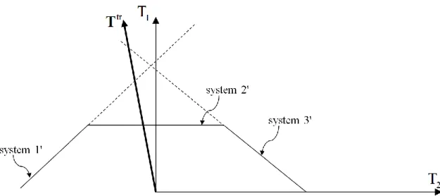
The remarks below rely on the fictitious yield surface introduced in Figure 2.
Remark 1: The first sub-increment of computation is elastic, as the single crystal is generally
assumed to be initially stress-free (i.e. (t = 0) =σ 0 ), and this sub-increment permits to catch the first facet of the yield surface, which corresponds to the activation of system 1'. As the crystal is loaded further, the stress state rides along the system 1', until it activates system 2'. In this
manner, other facets are progressively reached in the following sub-increments until arriving at a vertex of the yield surface (the intersection of at least 5 facets). Note that, during this process, some systems may be activated simultaneously. Generally, at this stage, only one sub-increment (for typical values of strain increments, which are about 0.1–1% in FE simulations) is required in order to reach the next facet. Therefore, for these first sub-increments (when the stress state is not yet located at a vertex of the yield surface), the explicit algorithm is used without implicit correction, as δt is generally smaller than Δt.
Remark 2: When the stress state at t is laid on a vertex, and unless changes in the loading path 0 or unloading occur, ed(t ) is an outward vector with respect to the yield surface. As the yield surface is convex, the stress remains constrained to this vertex, and it is impossible to reach a novel facet of the yield surface during the remainder of the time increment IΔ. Accordingly, there is no change in the set of potentially active slip systems in this case. This implies that δt is equal to Δt (see Eq. (73)), which means that the implicit correction is possible in this case. In order to geometrically illustrate the previous two remarks, a simplified 2D schematic representation of the single crystal yield surface is introduced in Figure 2. The idea behind the progression shown in Figure 2 can be easily extended to the general case of the single crystal yield surface (which is represented in the linear five-dimensional deviatoric space).
3.3. Derivation of an analytical expression for the consistent tangent modulus
For the sake of brevity, only the tangent modulus, consistent with the ultimate integration scheme, is derived in this section. For the return-mapping integration scheme, several versions of the consistent tangent modulus have been given (in a Lagrangian formulation) in [41] and [42].
In order to simplify the following developments, the time increment [t0, t0+t] is assumed to consist of
a single sub-increment. Accordingly, I (resp. t) is equal to I (resp. t). From a practical point of view, this assumption is generally valid after few time increments (usually starting from the third or the fourth time increment). When the time increment is composed of more than one sub-increment, the following development remains valid, provided it is applied to the last sub-increment of [t0, t0+t]. In
order to simplify notations, the argument t0+t is dropped in the following developments, with the
implied understanding that the corresponding variable is evaluated at t0+t.
In order to take the finite strain aspects into account (finite deformation as well as finite rotation), the consistent tangent modulus is computed in the co-rotational frame, where it is defined by the following expression (see, e.g., [4344]):
ep ˆ Δ ˆ ˆ Δ σ ε , (91)
in which ˆσ and ˆε represent, respectively, the Cauchy stress increment and the corresponding strain increment (equal to t ˆd, as ˆd is assumed to be constant over the time increment), both being
expressed in the co-rotational frame. This co-rotational frame is determined by the anti-symmetric part
w of the velocity gradient g . Then, the rotation tensor ˆr is defined as the orientation of the co-rotational frame relative to the fixed frame. This rotation has the following evolution law:
Δt 0 ˆ e w. (t )ˆ
r r . (92)
Any tensor X used in the current section will be denoted ˆX when expressed in the co-rotational frame.
To compute ˆ , the so-called secant modulusep ˆ , which relates the increment of the Cauchy stresss tensor ˆσ to the increment of the strain tensor ˆε, is first determined
s
ˆ
ˆ ˆ
Δσ : Δε. (93)
Indeed, the stress increment Δσˆ can be expressed as follows:
T 0
ˆ ˆ ˆ ˆ
Δσ σ σ (t )r σ r. . σ(t ), (94)
where r is the rotation of the intermediate configuration relative to the co-rotational frame. Its
evolution is defined by the following equation:
p αˆα ˆ Δt Δt γ 0 e w . (t ) e S. (t ) ; α r r r . (95)
Using the update equation (78)(1),Δσˆ can be rewritten as
T 0 0 0 T T T T 0 0 0 0 ˆ ˆ ˆ ˆ Δ (t ) .( (t ) Δt ). (t ) ˆ . (t )]. (t ).[ . (t )] Δt . . (t ). σ σ σ r σ σ r σ r r σ r r r σ r σ (96)
By using Eq. (95), r r. T(t )0 and [ .r rT(t )]0 T can be expressed as
αˆα α α Δt γ Δt γ T T T 0 . (t ) e S , [ . (t )] e ; α r r r r . (97)
For small time increments, tensor eΔt γα αSˆ (resp. eΔt γα αSˆ ) can be approximated by
αˆα
Δt γ
1 S (resp.
αˆα
Δt γ
1 S ), since the higher-order terms in Δt are negligible. Hence, Eq. (96) can be transformed into
T 0 0 0 T α α 0 α α 0 ˆ ˆ ˆ ˆ Δ (t ) .( (t ) Δt ). (t ) ˆ ˆ Δt γ ]. (t ).[ Δt γ ] Δt . . (t ) σ σ σ r σ σ r σ 1 σ 1 S r σ r σ ; α . (98)
![Table A.1. The numbering of the slip systems of a BCC single crystal according to [50]](https://thumb-eu.123doks.com/thumbv2/123doknet/7296956.208834/50.892.101.777.448.701/table-numbering-slip-systems-bcc-single-crystal-according.webp)


![Figure 2. Evolution of the stress state on a 2D schematic representation of the single crystal yield surface: (a) First sub-increment [0, t 1 ], which corresponds to a purely elastic phase, (b) Second sub-increment [t 1 , t 2 ], which corr](https://thumb-eu.123doks.com/thumbv2/123doknet/7296956.208834/75.892.111.779.104.562/figure-evolution-schematic-representation-crystal-increment-corresponds-increment.webp)