GPU Divergence: ANALYSIS AND REGISTER ALLOCATION

HAL Id: hal-01612523

https://hal.inria.fr/hal-01612523

Submitted on 6 Oct 2017

HAL is a multi-disciplinary open access

archive for the deposit and dissemination of sci-entific research documents, whether they are pub-lished or not. The documents may come from teaching and research institutions in France or abroad, or from public or private research centers.

L’archive ouverte pluridisciplinaire HAL, est destinée au dépôt et à la diffusion de documents scientifiques de niveau recherche, publiés ou non, émanant des établissements d’enseignement et de recherche français ou étrangers, des laboratoires publics ou privés.

GPU Divergence: ANALYSIS AND REGISTER

ALLOCATION

Diogo Sampaio

To cite this version:

Diogo Sampaio. GPU Divergence: ANALYSIS AND REGISTER ALLOCATION. Computer Science [cs]. 0008. �hal-01612523�

DIVERGÊNCIA EM GPU: ANÁLISES E

ALOCAÇÃO DE REGISTRADORES

DIOGO N. SAMPAIO

DIVERGÊNCIA EM GPU: ANÁLISES E

ALOCAÇÃO DE REGISTRADORES

Dissertação apresentada ao Programa de Pós-Graduação em Ciência da Computação do Instituto de Ciências Exatas da Univer-sidade Federal de Minas Gerais como req-uisito parcial para a obtenção do grau de Mestre em Ciência da Computação.

Orientador: Fernando Magno Quintão Pereira

Belo Horizonte

Março de 2013

DIOGO N. SAMPAIO

GPU DIVERGENCE: ANALYSIS AND REGISTER

ALLOCATION

Dissertation presented to the Graduate Program in Computer Science of the Fed-eral University of Minas Gerais in partial fulfillment of the requirements for the de-gree of Master in Computer Science.

Advisor: Fernando Magno Quintão Pereira

Belo Horizonte

March 2013

© 2013, Diogo N. Sampaio. Todos os direitos reservados.

Sampaio, Diogo N.

S192d GPU divergence: analysis and register allocation / Diogo N. Sampaio. — Belo Horizonte, 2013

xviii, 73 f. : il. ; 29cm

Dissertação (mestrado) — Federal University of Minas Gerais

Orientador: Fernando Magno Quintão Pereira 1. Compilers. 2. GPGPU. 3. Static Analysis. 4. Divergence. 5. Register Allocation.

6. Rematerialization. I. Título. CDU 519.6*33 (043)

Resumo

Uma nova tendência no mercado de computadores é usar unidades de processamento gráfico (GPUs)1 _{para acelerar tarefas paralelas por dados. Esse crescente interesse}

re-novou a atenção dada ao modelo de execução Single Instruction Multiple Data (SIMD). Máquinas SIMD fornecem uma tremenda capacidade computacional aos desenvolve-dores, mas programá-las de forma eficiente ainda é um desafio, particularmente devido a perdas de performance causadas por divergências de memória e de fluxo. Esses fenô-menos são consequências de dados divergentes. Dados divergentes são variáveis com mesmo nome mas valores diferentes entre as unidades de processamento. A fim de li-dar com os fenômenos de divergências, esta dissertação introduz uma nova ferramenta de análise de código, a qual chamamos Análise de Divergência com Restrições Afins. Desenvolvedores de programas e compiladores podem servir-se das informações de di-vergência com dois propósitos diferentes. Primeiro, podem melhorar a qualidade de programas gerados para máquinas que possuem instruções vetoriais, mesmo que essas sejam incapazes de lidar com divergências de fluxo. Segundo, podem otimizar progra-mas criados para placas gráficas. Para exemplificar esse último, apresentamos uma otimização para alocadores de registradores que, usando das informações geradas pelas análises de divergências, melhora a utilização da hierarquia de memória das placas grá-ficas. Testados sobre conhecidos benchmarks, os alocadores de registradores otimizados produzem código que é, em média, 29.70% mais rápido do que o código gerado por alocadores de registradores convencionais.

Palavras-chave: Linguagem de Programação, Compiladores, GPGPU, Analise Es-tática, Divergências, Alocação de Registradores, Rematerialização, SIMT, SIMD.

1_{Do inglês Graphics Processing Units}

Abstract

The use of graphics processing units (GPUs) for accelerating Data Parallel workloads is the new trend on the computing market. This growing interest brought renewed atten-tion to the Single Instrucatten-tion Multiple Data (SIMD) execuatten-tion model. SIMD machines give application developers tremendous computational power; however, programming them is still challenging. In particular, developers must deal with memory and control flow divergences. These phenomena stem from a condition that we call data divergence, which occurs whenever processing elements (PEs) that run in lockstep see the same variable name holding different values. To deal with divergences this work introduces a new code analysis, called Divergence Analysis with Affine Constraints. Application developers and compilers can benefit from the information generated by this analysis with two different objectives. First, to improve code generate to machines that have vector instructions but cannot handle control divergence. Second, to optimize GPU code. To illustrate the last one, we present register allocators that rely on divergence in-formation to better use GPU memory hierarchy. These optimized allocators produced GPU code that is 29.70% faster than the code produced by a conventional allocator when tested on a suite of well-known benchmarks.

Keywords: Programming Languages, Compilers, GPGPU, Static Analysis, Diver-gence, Register Allocation, Rematerialization, SIMT, SIMD.

List of Figures

1.1 Google Trends chart: CUDA and OpenCL popularity over time . . . 6

1.2 GPU and CPU performance over time . . . 7

1.3 GPU and CPU performance on FEKO . . . 8

1.4 GPU and CPU design comparison . . . 8

2.1 Two kernels written in C for CUDA . . . 15

2.2 Divergence analyses comparison . . . 20

3.1 Variables dependency . . . 23

3.2 Simple divergence analysis propagation . . . 23

3.3 Affine analysis propagation . . . 25

3.4 Execution trace of a µ-Simd program . . . 31

3.5 Program in GSA form . . . 32

3.6 Constraint system used to solve the simple divergence analysis . . . 34

3.7 Dependence graph created for the example program . . . 35

3.8 Constraint system used to solve the divergence analysis with affine con-straints of degree one . . . 38

3.9 Variables classified by the divergence analysis with affine constraints . . . . 39

3.10 Higher degree polynomial improves the analysis precision . . . 41

4.1 The register allocation problem for the kernel avgSquare in Figure 2.1 . . 46

4.2 Traditional register allocation, with spilled values placed in local memory . 47 4.3 Using faster memory for spills . . . 48

4.4 Register allocation with variable sharing. . . 49

5.1 Divergence analyses execution time comparison chart . . . 53

5.2 Affine analysis linear time growth . . . 54

5.3 Variables distribution defined by affine analysis . . . 55

5.4 Variables affine classification per kernel . . . 56 xiii

5.5 Chart comparing number of divergent variables reported . . . 57

5.6 Kernels speedup per register allocator . . . 59

5.7 Spill code distribution based on spilled variables abstract state . . . 60

5.8 Spill code affine state distribution per kernel . . . 61

List of Tables

3.1 The syntax of µ-Simd instructions . . . 27

3.2 Elements that constitute the state of a µ-Simd program . . . 27

3.3 The auxiliary functions used in the definition of µ-Simd . . . 28

3.4 The semantics of µ-Simd: control flow operations . . . 29

3.5 The operational semantics of µ-Simd: data and arithmetic operations . . . 30

3.6 Operation semantics in the affine analysis . . . 37

Contents

Resumo ix

Abstract xi

List of Figures xiii

List of Tables xv

1 Introduction 5

1.1 How important GPUs are becoming . . . 5

1.2 Divergence . . . 7

1.3 The problem of divergence . . . 9

1.4 Our contribution . . . 9

2 Related work 13 2.1 Divergence . . . 13

2.2 Divergence Optimizations . . . 16

2.2.1 Optimizing divergent control flow . . . 16

2.2.2 Optimizing memory accesses . . . 17

2.2.3 Reducing redundant work . . . 18

2.3 Divergence Analyses . . . 18

2.3.1 Chapter conclusion . . . 19

3 Divergence Analyses 21 3.1 Overview . . . 21

3.2 The Core Language . . . 26

3.3 Gated Static Single Assignment Form . . . 31

3.4 The Simple Divergence Analysis . . . 33

3.5 Divergence Analysis with Affine Constraints . . . 36 xvii

3.6 Chapter conclusion . . . 41

4 Divergence Aware Register Allocation 43 4.1 GPU memory hierarchy . . . 44

4.2 Adapting a Traditional Register Allocator to be Divergence Aware . . . 47

4.2.1 Handling multiple warps . . . 49

4.3 Chapter conclusion . . . 50 5 Experiments 51 5.1 Tests . . . 51 5.1.1 Hardware . . . 51 5.2 Benchmarks . . . 51 5.3 Results . . . 52 5.4 Chapter conclusion . . . 62 6 Conclusion 63 6.1 Limitations . . . 64 6.2 Future work . . . 65 6.3 Final thoughts . . . 66 Bibliography 67 xviii

CONTENTS 1

Glossary

GPU Graphics Processing Unit: Is a hardware accelerator. The first GPUs were built with specific purpose to accelerate the process of representing lines and arcs in bitmaps, to be displayed on the mon-itor. With time, GPUs incorporated hardware implementations of functions used to rasterize three dimensional scenarios. Later on, this accelerator turned to be massively parallel accelerators, capable of generic processing.

CUDA Compute Unified Device Architecture: Is a parallel

comput-ing platform and programmcomput-ing model created by NVIDIA and im-plemented to the graphics processing units (GPUs) that they pro-duce.

PTX Parallel Thread Execution: Is a pseudo-assembly language used in Nvidia’s CUDA programming environment. The nvcc compiler translates code written in CUDA, a C-like language, into PTX, and the graphics driver contains a compiler which translates the PTX into a binary code which can be run on the processing cores. Code hoisting Compiler optimizations techniques that reduce amount of

instruc-tions by moving duplicated instrucinstruc-tions on different execution paths to a single instructions on a common path.

kernel Function that executes in the GPU.

thread block Is a set of threads, defined by the programmer, at a kernel call. A thread blockexecutes in one SM, sharing its resources, such as cache memory and register file, equally among all threads of the block.

SM Stream Multiprocessor: A SIMD processor. It executes threads

of a thread block in warps.

warp A group of GPU threads that execute on lock-step.

threads Execution lines in the same kernel. GPU threads share global and shared memory, and have different mappings for the register file and local memory.

Acknowledgment

Many thanks to Sylvain Collange, Bruno Coutinho and Gregory Diamos for helping in the implementation of this work, to my adviser, Fernando Pereira, for being a source of inspiration and knowledge, and to my family, for the unconditional support and so much more that I can’t describe in words.

Chapter 1

Introduction

A new trend in the computer market is to use GPUs as accelerators for general purpose applications. This raising popularity stems from the fact that GPUs are massively par-allel. However GPUs impose new programming challenges onto application developers. These challenges are due, mostly to control and memory divergences. We present an new compiler analysis that identify divergence hazards and can help developers and automatic optimizations to generate faster GPU code. Our analysis can also assist the translation of GPU designed applications to vector instructions on conventional CPUs, that cannot handle divergence hazards.

1.1

How important GPUs are becoming

Increasing programmability and low hardware cost are boosting the use of GPUs as a tool to accelerate general purpose applications. This trend can be especially observed on the academic environment, as demonstrated in Google Trends1 _{and TOP 500}

super-computers. The chart 1.1, taken from Google Trends, illustrates the rising popularity of CUDA2 _{(see NVIDIA [2012]) and OpenCL}3 _{(see Khronos [2011]) languages among}

the Computer Science community. TOP 500 supercomputers, an organization that of-ten ranks the 500 most powerful supercomputers on the world, demonstrates that by November 2012 (see TOP500 [2012]), 53 of these supercomputers use GPUs accelera-tors, where three of them are among the five most power efficient (Mflops / watt) and

1_{http://www.google.com/trends/}

2_{Compute Unified Device Architecture: a parallel computing platform and programming model}

created by NVIDIA

3_{Open Computing Language: Open standard framework for writing programs that execute across}

heterogeneous platforms

6 Chapter 1. Introduction

04/08 04/09 04/10 04/11 04/12

CUDA

OpenCL

Figure 1.1. Google Trends chart: CUDA and OpenCL popularity over time

two among the ten most powerful.

This trend will continue, as academia and industry work on improving GPUs hardware and software. Efficient GPU algorithms were presented to solve problems as diverse as sorting (Cederman and Tsigas [2010]), gene sequencing (Sandes and de Melo [2010]), IP routing (Mu et al. [2010]) and program analysis (Prabhu et al. [2011]). Performance tests exposed by Ryoo et al. [2008] demonstrate that some programs can run over 100 times faster on GPUs than their CPU equivalent. Upcoming hardware will closely integrate GPUs and CPUs, as demonstrated by Boudier and Sellers [2011] and new models of heterogeneous hardware are being introduced (Lee et al. [2011]; Saha et al. [2009]).

GPUs are attractive because these processors are massively parallel and high through-put oriented. To illustrate GPUs characteristics, we are going to use NVIDIA’s GeForce GTX-580 GPU series, a domestic high-end GPU. A GTX-580 has 512 processing el-ements (PEs) that can be simultaneously used by up to 24,576 threads. It delivers, approximately, up to 1500 Gflops4 in single precision, much higher than the 62 Gflops

1.2. Divergence 7

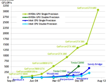
Figure 1.2. Chart taken from Nvidia’s CUDA C Programming Guide that shows GPU and CPU peak performance over time

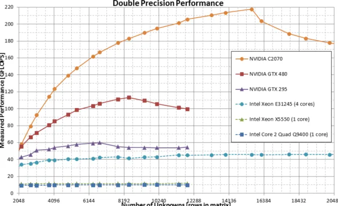
of a CPU at the same price range and release date. The chart 1.2 compares GPU to CPU theoretical computational power over time and 1.3 illustrates how domestic GPUs can outperform server CPUs when solving the same problem using FEKO5 _{, a}

parallel library for electromagnetic simulation.

Compared to a regular CPU, a GPU chip devotes much more transistors to PEs and much fewer transistors to cache memory and flow control, as illustrated by figure 1.4. To reduce dramatically their control hardware, GPUs adopt a more restrictive pro-gramming model, and not every parallel application can benefit from this parallelism. These processors organize threads in groups that execute in lock-step, called warps.

1.2

Divergence

To understand the rules that govern threads in a warp, we can imagine that each warp has simultaneous access to many PEs, but uses only one instruction fetcher. As an example, the GTX-580 has 16 independent cores, called Streaming Multiprocessors (SM). Each SM can run 48 warps of 32 threads each, thus, each warp might execute 32 instances of the same instruction simultaneously. Regular applications, such as Data parallel algorithms studied by Hillis and Steele [1986], fare very well in GPUs, as we

8 Chapter 1. Introduction

Figure 1.3. GPU and CPU performance on FEKO

Control Cache memory ALU

CPU GPU

Figure 1.4. GPU and CPU design comparison

have the same operation being independently performed on different chunks of data. However, divergence may happen in less regular applications.

Definition 1(Data divergence). Data divergence happens whenever the same variable name is mapped to different values by different threads. In this case we say that the variable is divergent, otherwise we call it uniform.

As we will see in chapter 2, a thread identifier (Tid) for instance, a special variable that

1.3. The problem of divergence 9

1.3

The problem of divergence

Data divergencesare responsible for two phenomena that can compromise performance: memory and control flow divergence. Control flow divergence happens when threads in a warp follow different paths after processing the same branch instruction. If the branching condition is data divergent, then it might be true to some threads, and false to others. The code from both paths, following the branch instruction, is serialized. Given that each warp has access to only one instruction at a time some threads have to wait idly, while others execute. As pointed out by Zhang et al. [2011], in a worse case scenario, control flow divergence can reduce hardware utilization down to 3, 125% on a GTX-580, when only one among all 32 threads of a warp is active.

Memory divergence, a term coined by Meng et al. [2010], happens whenever a load or store instruction targeting data divergent addresses causes threads in a warp to access memory positions with bad locality. Usually each thread request a different memory position upon a input data access. Such event request that a huge amount of data to travel between memory and the GPU. To deal with these events GPUs rely on a very large memory communication bandwidth, being able to transfer a huge amount of data at once. However, the data requested need to be congruent to be transferred at once. If the memory access requested by a single instruction is apart by more than the memory communication bandwidth, more than one memory access is required to deliver the requested data of a single instruction. If each thread access a data that is very distant apart from each other, a single instruction could generate many memory transfers. Such events have been shown by Lashgar and Baniasadi [2011] to have even more performance impact than control flow divergence.

Optimizing an application to avoid divergence is problematic for two reasons. First, some parallel algorithms are intrinsically divergent; thus, threads will naturally disagree on the outcome of branches. Second, identifying divergences burdens the application developer with a tedious task, which requires a deep understanding of code that might be large and complex.

1.4

Our contribution

Our main goal is to provide compilers with techniques that allow them to understand and to improve divergent code. To meet such objective in Section 3.4 we present a static program analysis that identifies data divergence. We then expand this analysis, discussing, in Section 3.5, a more advanced algorithm that distinguishes divergent and

10 Chapter 1. Introduction affinevariables, e.g. variables that are affine expressions of thread identifiers. The two analyses discussed here rely on the classic notion of Gated Static Single Assignment form(see Ottenstein et al. [1990]; Tu and Padua [1995]), which we revise in Section 3.3. We formalize our algorithms by proving their correctness with regard to µ-Simd, a core language that we describe in Section 3.2.

The divergence analysis is important in different ways. Firstly, it helps the compiler to optimize the translation of Single Instruction Multiple Threads (SIMT6_{, see Patterson}

and Hennessy [2012]; Garland and Kirk [2010]; Nickolls and Dally [2010]; Habermaier and Knapp [2012]) languages to ordinary CPUs. We call SIMT languages those pro-gramming languages, such as C for CUDA and OpenCL, that are equipped with ab-stractions to handle divergence. Currently there exist many proposals (Diamos et al. [2010]; Karrenberg and Hack [2011]; Stratton et al. [2010]) to compile such languages to ordinary CPUs and they all face similar difficulties. Vector operations found in traditional architectures, such as the x86’s SSE extension, do not support control flow divergence natively. Different than GPUs, where each data is processed by a different thread, that can be deactivated upon a control flow divergence, these instructions are executed by a single thread, that do the same operation on all data of a vector. If different data on a single vector need to be submitted to different instructions, these vector need to be reorganized on vector that all elements need to be submitted to the same treatment. Such problems have been efficiently addressed by Kerr et al. [2012], but still requires extra computation at thread frontier to recalculate active threads. This burden can be safely removed from the uniform, e.g., non-divergent, branches that we identify. Furthermore, the divergence analysis provides insights about memory access patterns, as demonstrated by Jang et al. [2010]. In particular, a uniform address means that all threads access the same location in memory, whereas an affine address means that consecutive threads access adjacent or regularly-spaced memory locations. This information is critical to generate efficient code for vector instruction sets that do not support fast memory gather and scatter (see Diamos et al. [2010]).

Secondly, in order to more precisely identify divergence, a common strategy is to use instrumentation based profilers. Coutinho et al. [2010] has done so, however, this approach may slowdown the target program by factors of over 1500 times! Our di-vergence analysis reduces the amount of branches that the profiler must instrument; hence, decreasing its overhead.

Thirdly, the divergence analysis improves the static performance prediction techniques

1.4. Our contribution 11

used in SIMT architectures (see Baghsorkhi et al. [2010]; Zhang and Owens [2011]). For instance, Samadi et al. [2012] used adaptive compilers that target GPUs.

Finally, our analysis also helps the compiler to produce more efficient code to SIMD hardware. There exists a recent number of divergence aware code optimizations, such as Coutinho et al. [2011] branch fusion, and Zhang et al. [2011] thread reallocation strategy. We augment this family of techniques with a divergence aware register alloca-tor. As shown in Chapter 4, we use divergence information to decide the best location of variables that have been spilled during register allocation. Our affine analysis is specially useful to this end, because it enables us to perform Rematerialization (see Briggs et al. [1992]) of values among SIMD processing elements. Rematerialization is a compiler optimization which saves time by recomputing a value instead of loading it from memory. It is typically tightly integrated with register allocation, where it is used as an alternative to spilling registers to memory.

All the algorithms that we describe are publicly available in the Ocelot compiler7

(Diamos et al. [2010]). Our implementation in the Ocelot compiler consists of over 10,000 lines of open source code. Ocelot optimizes PTX code, the intermediate program representation used by NVIDIA’s GPUs. We have compiled all the 177 CUDA kernels8

from 46 applications taken from the Rodinia (Che et al. [2009]) and the NVIDIA SDK benchmarks. The experimental results given in Section 5 show that our implementation of the divergence analysis runs in linear time on the number of variables in the source program. The basic divergence analysis proves that about one half of the program variables, on average, are uniform. The affine constraints from Section 3.5 increase this number by 4%, and – more important – they indicate that about one fourth of the divergent variables are affine functions of some thread identifier. Finally, our divergence aware register allocator is effective: by rematerializing affine values, or moving uniform values to the GPU’s shared memory, we have been able to speedup the code produced by Ocelot’s original allocator by almost 30%.

As a result of this research the following papers were published: • Spill Code Placement for SIMD Machines

Best paper award

Sampaio, D. N., Gedeon, E., Pereira, F. M. Q., Collange, S.

16th Brazilian Symposium, SBLP 2012, Natal, Brazil, September 23-28, 2012 Programming Languages, pp 12-26, Springer Berlin Heidelberg.

7_{Available at http://code.google.com/p/gpuocelot/}

12 Chapter 1. Introduction • Divergence Analysis with Affine Constraints

Sampaio, D. N., Martins, R., Collange, S., Pereira, F. M. Q.

24th International Symposium on Computer Architecture and High Performance Computing, New York City, USA

Chapter 2

Related work

Although General Purpose GPU (GPGPU) programming is a recent technology, it is rapidly becoming popular, especially on the scientific community. A substantial body of work has been published about program optimizations that target GPUs specifi-cally. The objective of this chapter is to discuss the literature that has been produced about compiler optimizations for GPUs. Therefore we further detail divergences via an example (Section 2.1), give notations on divergence optimizations (Section 2.2) and compare our divergence analysis against previous work.

2.1

Divergence

GPUs run in the so called SIMT execution model. The SIMT model combines MIMD, SPMD and SIMD semantics, but divergence is relevant only at the SIMD level. This semantics combination works as follows:

• Each GPU might have one or more cores (SM), that follow Flynn’s Multiple Instruction Multiple Data (MIMD) model (see Flynn [1972]), that is, each SM can be assigned to execute code from a different kernel and SMs executing code from the same kernel are not synchronized.

• Threads from the same kernel are grouped in Thread Blocks. Each Thread Block is assigned to a SM. Each Thread Block is divided in fixed sets of threads called warps. Each warp in a Thread Block follows Darema’s Single Program Multiple Data (SPMD) execution model (Darema et al. [1988]), that is, within a Thread Block all warps execute the same kernel but are scaled asynchronously.

14 Chapter 2. Related work • Threads inside the same warp execute in lock-step, fitting Flynn’s SIMD ma-chines, that is, all threads of a warp execute simultaneously the same instruction.

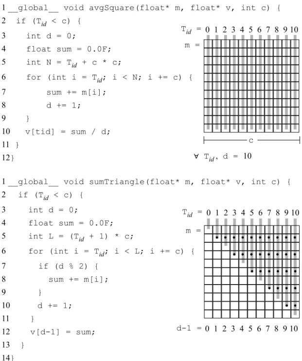
We will use two artificial programs in Figure 2.1 to explain the notion of divergence. These functions, normally called kernels, are written in C for CUDA and run on graph-ics processing units. We will assume that these programs are executed by a number of threads, or PEs, according to the SIMD semantics. All the PEs see the same set of variable names; however, each one maps this environment onto a different address space. Furthermore, each PE has a particular set of identifiers. In C for CUDA this set includes the index of the thread in three different dimensions, e.g., threadIdx.x, threadIdx.y and threadIdx.z. We will denote this unique thread identifier by Tid.

Each thread uses its Tid to find the data that it must process. Thus, in the kernel

avgSquareeach thread Tid is in charge of adding the elements of the Tid-th column of

m. Once leaving the loop, this thread will store the column average in v[Tid]. This is a

divergent memory access: each thread will access a different memory address. However, modern GPUs can perform these accesses very efficiently, because they have good locality. In this example, addresses used by successive threads are contiguous (Ryoo et al. [2008]; Yang et al. [2010]). Control flow divergence will not happen in avgSquare. That is, each thread will loop the same number of times. Consequently, upon leaving the loop, every thread sees the same value at its image of variable d. Thus, we call this variable uniform.

Kernel sumTriangle presents a very different behavior. This rather contrived function sums up the columns in the superior triangle of matrix m; however, only the odd lines of a column contribute to the sum. In this case, the threads perform different amounts of work: the threads that has Tid= nwill visit n+1 cells of m. After a thread leaves the

loop, it must wait for the others. Processing resumes once all of them synchronize at line 12. At this point, each thread sees a different value stored at its image of variable d, which has been incremented Tid+ 1times. Hence, we say that d is a divergent variable

outside the loop. Inside the loop, d is uniform, because every active thread sees the same value stored at that location. Thus, all the threads active inside the loop take the same path at the branch in line 7. Therefore, a precise divergence analysis must split the live range of d into a divergent and a uniform part.

2.1. Divergence 15

1 __global__ void avgSquare(float* m, float* v, int c) { 2 if (T_id < c) { 3 int d = 0; 4 float sum = 0.0F; 5 int N = T_id + c * c; 6 for (int i = T_id; i < N; i += c) { 7 sum += m[i]; 8 d += 1; 9 } 10 v[tid] = sum / d; 11 } 12}

1 __global__ void sumTriangle(float* m, float* v, int c) { 2 if (T_id < c) { 3 int d = 0; 4 float sum = 0.0F; 5 int L = (T_id + 1) * c; 6 for (int i = T_id; i < L; i += c) { 7 if (d % 2) { 8 sum += m[i]; 9 } 10 d += 1; 11 } 12 v[d-1] = sum; 13 } 14} c 0 1 2 3 4 5 6 7 8 9 10 T_id = m = ∀ T_id , d = 10 0 1 2 3 4 5 6 7 8 9 10 T_id =

• • • • • • • • •

• • • • • • •

• • • • •

• • •

•

d-1 = 0 1 2 3 4 5 6 7 8 9 10 m =

•

•

•

•

•

Figure 2.1. The gray lines on the right show the parts of matrix m processed by each thread. Following usual coding practices we represent the matrix in a linear format. Dots mark the cells that add up to the sum in line 8 of sumTriangle.

16 Chapter 2. Related work

2.2

Divergence Optimizations

We call divergence optimizations the code transformation techniques that use the re-sults of divergence analysis to generate better programs. Some of these optimizations deal with memory divergences; however, methods dealing exclusively with control flow divergence are the most common in the literature. As an example, the PTX program-ming manual1 _{recommends replacing ordinary branch instructions (bra) proved to be}

non-divergent by special instructions (bra.uni), which are supposed to divert control to the same place for every active thread. Other examples of control flow divergence optimizations include branch distribution, branch fusion, branch splitting, loop collaps-ing, iteration delaying and thread reallocation. At run-time divergence control flow can be reduced with a more complex hardware as demonstrated in large warps and two-level warp schedulingand SIMD re-convergence at thread frontiers.

2.2.1

Optimizing divergent control flow

A common method to optimize divergent control flow is to minimize the amount of work done in divergent paths, such as branch distribution and branch fusion.

Branch distribution (Han and Abdelrahman [2011]) is a form of code hoisting2 that works both at the Prolog and at the epilogue of a branch. This optimization merges code from potentially divergent paths to outside the branch. Branch fusion (Coutinho et al. [2011]), a generalization of Branch distribution, joins chains of common instruc-tions present in two divergent paths if the additional execution costs of regenerating the same divergence is lower than the potential gain.

A number of compiler optimizations try to rearrange loops in order to mitigate the impact of divergence. Carrillo et al. [2009] proposed branch splitting, a way to divide a parallelizable loop enclosing a multi-path branch into multiple loops, each containing only one branch. Lee et al. [2009] designed loop collapsing, a compiler technique that reduces divergence inside loops when compiling OpenMP programs into C for CUDA. Han and Abdelrahman [2011] generalized Lee’s approach proposing iteration delaying, a method that regroups loop iterations, executing those that take the same branch direction together.

Thread reallocationis a technique that applies on settings that combine the SIMD and

1_{PTX programming manual, 2008-10-17, SP-03483-001_v1.3, ISA 1.3}

2 _{techniques known as code hoisting tend to diminish the number of instructions of a program by}

unifying duplicated instructions on different control flow paths into a unique instruction in a common path

2.2. Divergence Optimizations 17

the SPMD semantics, like the modern GPUs. This optimization consists in regrouping divergent threads among warps, so that only one or just a few warps will contain divergent threads. Their main idea is that divergence occur based on input values, so they sort the input vectors applying the same modification over the threadIdx. It has been implemented at the software level by Zhang et al. [2010, 2011], and simulated at the hardware level by Fung et al. [2007]. However, this optimization must be used with moderation, as shown by Lashgar and Baniasadi [2011], unrestrained thread regrouping could lead to memory divergence.

At the hardware level, Narasiman et al. [2011] propose in Improving GPU performance via large warps and two-level warp scheduling warps with number of threads multiple of number of PEs in a Stream Multiprocessor by a factor n. A inner warp scheduler is capable of selecting for each PE, one among n threads, always preferring an active. Such mechanism can reduce the number of inactive threads selected for execution, but it also can lead to memory divergence.

Most GPUs only converge execution of divergent threads at the post-dominator block of divergent branches. Diamos et al. [2011] in SIMD re-convergence at thread frontiers minimize the amount of time that threads remain inactive by using a hardware capable of identifying blocks before the post dominator, called thread frontiers, where some threads of a warp might resume execution. The active threads set is recalculated at these points comparing the current PC against the PC of inactive threads.

2.2.2

Optimizing memory accesses

The compiler related literature describes optimizations that try to change memory access patterns in such a way to improve address locality. Recently, some of these techniques were adapted to mitigate the impact of memory divergence in modern GPUs. Yang et al. [2010] and Pharr and Mark [2012] describe a suite of loop transformations to coalesce data accesses. Memory coalescing consists in the dynamic aggregation of contiguous locations into a single data access. Leissa et al. [2012] discuss several data layouts that improve memory locality in the SIMD execution model.

Rogers et al. [2012] propose in Cache-Conscious Wavefront Scheduling a novel warp scheduler that uses a scoreboard based on the warp memory access pattern and data stored in cache, being able to maximize L1 data cache reuse among warps of a thread block, archiving a 24% performance gain over the previous state of the art warp sched-uler.

18 Chapter 2. Related work

2.2.3

Reducing redundant work

The literature describes a few optimizations that use data divergence information to reduce the amount of work that the SIMD processing elements do. For instance, Collange et al. [2010] introduces work unification. This compiler technique leaves to only one thread the task of computing uniform values; hence, reducing memory accesses and hardware occupancy. Some computer architectures, such as Intel MIC3 _{and AMD}

GCN4_{, combine scalar and SIMD processing units. Although we are not aware of}

any work that tries to assign computations to the different units based on divergence information, we speculate that this is another natural application of the analysis that we present.

2.3

Divergence Analyses

Several algorithms have been proposed to find uniform variables. The first technique that we are aware of is the barrier inference of Aiken and Gay [1998]. This method, designed for SPMD machines, finds a conservative set of uniform5 variables via static

analysis. However, because it is tied to the SPMD model, Aiken and Gay’s algorithm can only report uniform variables at global synchronization points.

The recent interest on graphics processing units has given a renewed impulse to this type of analysis, in particular with a focus on SIMD machines. For instance, Stratton et al. [2010] variance analysis, and Karrenberg and Hack [2011] vectorization analysis distinguish uniform and divergent variables. However, these analyses are tools used in the compilation of SPMD programs to CPUs with explicit SIMD instructions, and both compilers generate specific instructions to manage divergence at run-time. On the other hand, we focus on architectures in which divergence are managed implicitly by the hardware. A naive application of Stratton’s and Karrenberg’s approach in our static context may yield false negatives due to control dependency, although they work well in the dynamic scenario for which they were designed. For instance, Karrenberg’s select and loop-blending functions are similar to the γ and η functions that we discuss in Section 3.3. However, select and blend are concrete instructions emitted during code generation, whereas our GSA functions are abstractions used statically.

Coutinho et al. [2011] proposed a divergence analysis that works in programs in the Gated Static Single Assignment (GSA) format (see Ottenstein et al. [1990]; Tu and

3_{See Many Integrated Core Architecture at http://www.intel.com. Last visit: Jan. 13} 4_{See Understanding AMD’s Roadmap at http://www.anandtech.com/. Last visit: Jan. 13} 5_{Aiken and Gay would call these variables single-valued}

2.3. Divergence Analyses 19

Padua [1995]). Thus, Coutinho et al.’s analysis is precise enough to find out that vari-able d is uniform inside the loop in the kernel sumTriangle, and divergent outside. Nevertheless, their version is over-conservative because it does not consider affine re-lations between variables. For instance, in the kernel avgSquare, variables i and L are functions of Tid. However, if we inspect the execution trace of this program, then

we will notice that the comparison i < L has always the same value for every thread. This fact happens because both variables are functions of two affine expressions of Tid,

whose combination cancel the Tid factor out, e.g.: L = Tid+ c1 and i = Tid+ c2; thus,

L − i = (1 − 1)Tid + (c1− c2). Therefore, a more precise divergence analysis requires

some way to take affine relations between variables into consideration.

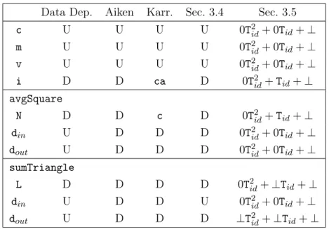
Figure 2.2 summarizes this discussion comparing the results produced by these different variations of the divergence analysis when applied on the kernels in Figure 2.1. We call Data Dep. a divergence analysis that takes data dependency into consideration, but not control dependency. In this case, a variable is uniform if it is initialized with constants or broadcast values, or, recursively, if it is a function of only uniform variables. This analysis would, incorrectly, flag variable d in avgSquare, as uniform. Notice that, because this analysis use the GSA intermediate representation, they distinguish the live ranges of variable d inside (din) and outside (dout) the loops. The analysis that we

present in Section 3.5 improves on the analysis that we discuss in Section 3.4 because it considers affine relations between variables. Thus, it can report that the loop in avgSquare is non-divergent, by noticing that the comparison i < N has always the same value for every thread. This fact happens because both variables are functions of two affine expressions of Tid, whose combination cancel the Tid factor out, e.g.:

N = Tid+ c1 and i = Tid+ c2; thus, N − i = (1 − 1)Tid + (c1− c2).

2.3.1

Chapter conclusion

This chapter provided some context on which the reader can situate himself. It defined divergence data, and showed this kind of data can degrade the performance of a GPU, via flow and memory divergences. It described possible optimizations that can ben-efit from the information of divergence analysis as motivation for our new technique, comparing its results against previously proposed techniques. As we will explain in the rest of this dissertation, our divergence analysis is more powerful than the previous approaches, because it relies on a more complex lattice. The immediate result is that we are able to use it to build a register allocator that would not be possible using only the results of the other techniques that have been designed before ours. In the next chapter we formalize our notion of divergence analysis with affine constraints.

20 Chapter 2. Related work

Data Dep. Aiken Karr. Sec. 3.4 Sec. 3.5

c U U U U 0T2_id+ 0Tid+ ⊥ m U U U U 0T2_id+ 0Tid+ ⊥ v U U U U 0T2_id+ 0Tid+ ⊥ i D D ca D 0T2_id+ Tid+ ⊥ avgSquare N D D c D 0T2_id+ Tid+ ⊥ din U D D D 0T2id+ 0Tid+ ⊥ dout U D D D 0T2_id+ 0Tid+ ⊥ sumTriangle L D D D D 0T2_id+ ⊥Tid+ ⊥ din U D D U 0T2id+ 0Tid+ ⊥ dout U D D D ⊥T2_id+ ⊥Tid+ ⊥

Figure 2.2. We use U for uniform and D for Divergent variables. Karrenberg’s analysis can mark variables in the format 1 × Tid+ c, c ∈ N as consecutive (c) or

Chapter 3

Divergence Analyses

In this chapter we describe two divergence analyses. We start by giving in Section 3.1 an informal overview on the basics of divergence analysis. We describe how our technique of using affinity with the Tid augments the precision compared to a simple

implementa-tion. In Section 3.4 we formalize a simple and fast implementaimplementa-tion. This initial analysis helps us to formalize the second algorithm, presented in Section 3.5, a slower, yet more precise technique because it can track affine relations between program variables, an extra information vital to our novel register allocator. Our affine divergence aware register allocator uses the GPU’s memory hierarchy in a better way when compared to previous register allocators. This better usage comes out of the fact that our allocator decreases the amount of memory used when affine variables are selected for spilling. It does so by trading memory space by extra computations, which we perform as value rematerialization. We formalize our divergence analysis by describing how it operates on a toy SIMD model, which we explain in Section 3.2. Our analysis requires the com-piler to convert the target program to a format called Gated Static Single Assignment form. We describe this format in Section 3.3.

3.1

Overview

Divergence Analyses, in the GPU context, are compiler static analyses that classify variables accordingly to, either all threads will see it with the same value or not. As in the Definition 1, the conservative set of variables classified as uniform variables will hold variables that, at compile time, are known to contain the same value among all threadsat run-time. The set of divergent variables hold the variables that might contain different values among threads at run-time.

22 Chapter 3. Divergence Analyses To be able to classify variables as divergent and uniform, divergence analysos rely on:

1. Data divergence origins are known at compile time, and are pre-classified as di-vergent variables. Divergence origins are:

a) Threads identifiers (Tid): It is known to be a unique value per thread.

b) Atomic operations results: Each thread might receive a different value after an atomic operation.

c) Local Memory Loads: Local memory has a unique mapping per thread, so values loaded from it might be different among threads.

2. Divergent variables can only affect variables that dependent on them. There are two types of dependency among variables:

a) Data dependency. b) Control dependency.

Variables dependency are represented in a oriented graph. If a variable v is depen-dent on the variable Tid, then there is an arrow from Tid to v. Data dependency is

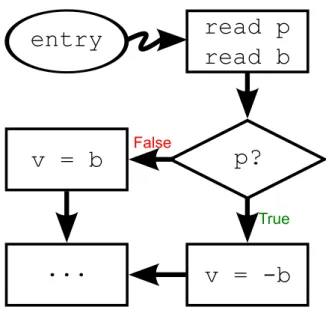
easily extracted from the instructions of the program. To every instruction, such as a = b + c, the left side (a) is dependent on the right side (b, c). Control dependency is a little more tricky to be detected, and require a special program representation to be identified, as described in details in Section 3.3. But a simple definition is, if variable p controls which value is assigned to a variable v, then v is control dependent on p. The fluxogram in Figure 3.1 illustrates data and control dependency.

3.1. Overview 23

read p

read b

entry

p?

v = b

v = -b

...

True False

Figure 3.1. Variable v is data dependent of variable b and control depen-dent of variable p.

The simple divergence analysis builds the variable dependency graph and uses a graph reachability algorithm to detect all variables dependent on divergent variables, as illustrated in Figure 3.2. c d k f _l h s i Tid Bid e 1 Bsz p c d k f _l h s i Tid Bid e 1 Bsz p

Figure 3.2. On the left the initial state of the variable dependency graph. On the right, variables states after graph reachability applied from divergence sources

24 Chapter 3. Divergence Analyses The divergence analysis with affine constraints is capable do give more details about the nature of the values that are going to be store in the variables. It uses the technique to keep variables affinity of degree one to the Tid. That is, all variables have

an abstract state, compound by two elements (a, b) that describe the encountered value as a × Tid+ b. Each of this elements can be assigned three possible values:

• >: The analysis did not process the affinity of the variable. • c: A constant value that is known at compile time.

• ⊥: At compile time is not possible to define any information about the factor. Based on these possible element states, all possible abstract states are:

• (>, >): The variable is still not processed by the analysis.

• (0, c): The variable is uniform and will hold a constant value that is known at compile time.

• (0, ⊥): The variable is uniform, but the value is not known at compile time. • (c1, c2): The variable is divergent, but we name it as affine because it is possible

to track the affinity with Tid. It is possible to the compiler use the constants c1

and c2 to write instructions that rematerialize the variable value.

• (c1, ⊥): The variable is divergent, but we name it as affine because it is possible

to track the affinity with Tid. It is possible to the compiler use the constant c and

a uniform variable to write instructions that rematerialize the variable value. • (⊥, ⊥): The variable is divergent or no information about the value at run-time

is known during compilation.

The affine technique rely on a dependency graph that takes into consideration the operations among variables, and uses different propagation rules to determine the out-put abstract state based on the inout-put ones. Special GPU variables, such as Tid, results

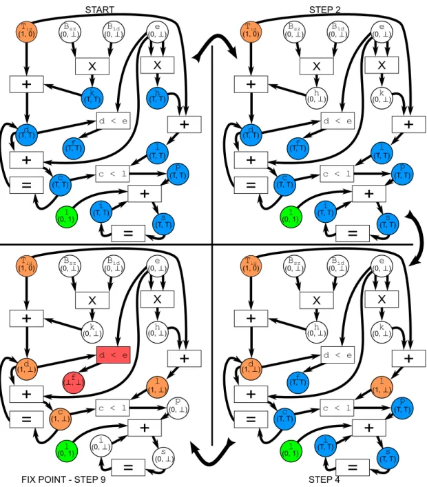
of atomic instructions, constant values, kernel parameters have their values statically predefined. All variables that have their abstract state predefined are inserted in the work-list. For each variable in the work-list we remove it and use propagation rules to compute the abstract state of all variables that depend on it. Always that the abstract state of a variable is altered, that variable is included in the work-list. We iterate until

3.1. Overview 25

the work-list is empty and the graph reach a fixed-point. Figure 3.3 demonstrates this process. c d k f _l h s i Tid (1, 0) Bid e X

+

d < e X

=

+

+

1 c < l

+

=

Bsz (0, ⊥) (0, ⊥) (0, ⊥) (T, T) (T, T) (T, T) (T, T) (T, T) (T, T) p (T, T) (T, T) (T, T) (0, 1) c d f _l s i Tid (1, 0) Bid e X

+

d < e X

=

+

+

1 c < l

+

=

Bsz (0, ⊥) (0, ⊥) (0, ⊥) (T, T) (T, T) (T, T) (T, T) p (T, T) (T, T) (T, T) (0, 1) k (0, ⊥) h (0, ⊥) START STEP 2 c d f _l h s i Tid (1, 0) Bid e X

+

d < e X

=

+

1 c < l

+

=

Bsz (0, ⊥) (0, ⊥) (0, ⊥) (0, ⊥) (1, ⊥) k (0, ⊥) (1, ⊥) (⊥, ⊥) (1, ⊥) p (0, ⊥) (0, ⊥) (0, ⊥) (0, 1) c f s i Tid (1, 0) Bid e X

+

d < e X

=

+

+

1 c < l

+

=

Bsz (0, ⊥) (0, ⊥) (0, ⊥) (T, T) (T, T) p (T, T) (T, T) (T, T) (0, 1) k (0, ⊥) h (0, ⊥) l (1, ⊥) d (1, ⊥) STEP 4 FIX POINT - STEP 9

+

Figure 3.3. On the top left the initial state of the variable dependency graph. Blue variables have a undefined abstract state. Especial variables, such as Tid, Bid

and Bsz, constants, such as 1, and function arguments, such as e, have predefined

abstract states. From these variables the state of all others are defined.

Now that we described how both techniques of divergence analysis work, we are going to prove and formalize its correctness. In Section 3.2 we introduce µ-Simd, a tool

26 Chapter 3. Divergence Analyses language that describes the rules followed by threads that execute in a same warp. In Section 3.3 we demonstrate how we transform our program CFG so it can inform control dependencies. In Section 3.4 we prove the Simple Divergence technique, as it help us to prove the correctness of our Affine Divergence Analysis in Section 3.5.

3.2

The Core Language

In order to formalize our theory, we adopt the same model of SIMD execution inde-pendently described by Bougé and Levaire [1992] and Farrell and Kieronska [1996]. We have a number of PEs executing instructions in lock-step, yet subject to partial execution. In the words of Farrel et al., “All processing elements execute the same statement at the same time with the internal state of each processing element being ei-ther active or inactive." [Farrell and Kieronska, 1996, p.40]. The archetype of a SIMD machine is the ILLIAC IV Computer (see Bouknight et al. [1972]), and there exist many old programming languages that target this model (Abel et al. [1969]; Bouknight et al. [1972]; Brockmann and Wanka [1997]; Hoogvorst et al. [1991]; Kung et al. [1982]; Lawrie et al. [1975]; Perrott [1979]). The recent developments in graphics cards brought new members to this family. The SIMT execution model is currently implemented as a multi-core SIMD machine – CUDA being a framework that coordinates many SIMD processors. We formalize the SIMD execution model via a core language that we call µ-Simd, and whose syntax is given in Table 3.1. We do not reuse the formal semantics of Bougé et al. or Farrell et al. because they assume high-level languages, whereas our techniques are better described at the assembly level. Notice that our model will not fit vector instructions, popularly called SIMD, such as Intel’s MMX and SSE exten-sions, because they do not support partial execution, rather following the semantics of Carnegie Mellon’s Vcode (Blelloch and Chatterjee [1990]). An interpreter for µ-Simd, written in Prolog, plus many example programs, are available in our web-page1_.

We define an abstract machine to evaluate µ-Simd programs. The state M of this machine is determined by a tuple with five elements: (Θ, Σ, Π, P, pc), which we define in Table 3.2. A processing element is a pair (t, σ), uniquely identified by the natural t, referred by the special variable Tid. The symbol σ represents the PE’s local memory,

a function that maps variables to integers. The local memory is individual to each PE; however, these functions have the same domain. Thus, v ∈ σ denotes a vector of variables, each of them private to a PE. PEs can communicate through a shared array Σ. We use Θ to designate the set of active PEs. A program P is a map of

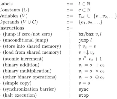
3.2. The Core Language 27 Labels ::= _{l ⊂ N} Constants (C) ::= _{c ⊂ N} Variables (V ) ::= Tid ∪ {v1, v2, . . .} Operands (V ∪ C) ::= {o1, o2, . . .} Instructions ::=

– (jump if zero/not zero) | bz/bnz v, l – (unconditional jump) | jump l – (store into shared memory) | ↑ vx = v

– (load from shared memory) | v =↓ vx

– (atomic increment) | v←− va x+ 1

– (binary addition) | v1= o1+ o2

– (binary multiplication) | v1= o1× o2

– (other binary operations) | v1= o1⊕ o2

– (simple copy) | v = o

– (synchronization barrier) | sync

– (halt execution) | stop

Table 3.1. The syntax of µ-Simd instructions

(Local memory) _{σ ⊂ Var 7→ Z} (Shared vector) _{Σ ⊂ N 7→ Z} (Active PEs) _{Θ ⊂ (N × σ)} (Program) P ⊂ Lbl 7→ Inst

(Sync stack) Π ⊂ Lbl × Θ × Lbl × Θ × Π

Table 3.2. Elements that constitute the state of a µ-Simd program

labels to instructions. The program counter (pc) is the label of the next instruction to be executed. The machine contains a synchronization stack Π. Each node of Π is a tuple (lid, Θdone, lnext, Θtodo)that denotes a point where divergent PEs must synchronize.

These nodes are pushed into the stack when the PEs diverge in the control flow. The label lid denotes the conditional branch that caused the divergence, Θdone are the PEs

that reached the synchronization point, whereas Θtodo are the PEs waiting to execute.

The label lnext indicates the instruction where Θtodo will resume execution.

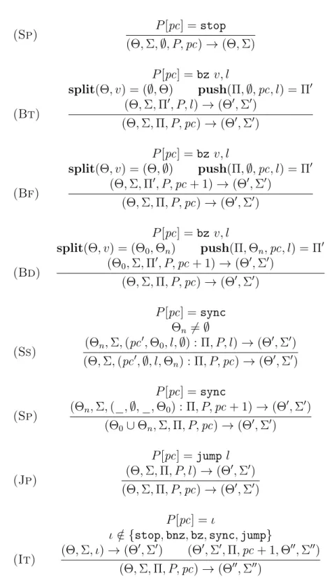
The result of executing a µ-Simd abstract machine is a pair (Θ, Σ). Figure 3.2 de-scribes the big-step semantics of instructions that change the program’s control flow. A program terminates if P [pc] = stop. The semantics of conditionals is more elabo-rate. Upon reaching bz v, l we evaluate v in the local memory of each active PE. If σ(v) = 0for every PE, then Rule Bf moves the flow to the next instruction, i.e., pc +1. Similarly, if σ(v) 6= 0 for every PE, then in Rule Bt we jump to the instruction at P [l]. However, if we get distinct values for different PEs, then the branch is divergent.

28 Chapter 3. Divergence Analyses split(Θ, v) = (Θ0, Θn) where Θ0 = {(t, σ) | (t, σ) ∈ Θ and σ[v] = 0} Θn= {(t, σ) | (t, σ) ∈ Θ and σ[v] 6= 0} push([], Θn, pc, l) = [(pc, [], l, Θn)] push((pc0, [], l0, Θ0_n) : Π, Θn, pc, l) = Π0 if pc 6= pc0 where Π0 = (pc, [], l, Θn) : (pc0, [], l0, Θ0n) : Π push((pc, [], l, Θ0_n) : Π, Θn, pc, l) = (pc, [], l, Θn∪ Θ0n) : Π

Table 3.3. The auxiliary functions used in the definition of µ-Simd

In this case, in Rule Bd we execute the PEs in the “then" side of the branch, keeping the other PEs in the sync-stack to execute them later. Stack updating is performed by the push function in Figure 3.3. Even the non-divergent branch rules update the synchronization stack, so that, upon reaching a barrier, i.e, a sync instruction, we do not get stuck trying to pop a node. In Rule Ss, if we arrive at the barrier with a group Θn of PEs waiting to execute, then we resume their execution at the “else"

branch, keeping the previously active PEs into hold. Finally, if we reach the barrier without any PE waiting to execute, in Rule Sp we synchronize the “done" PEs with the current set of active PEs, and resume execution at the next instruction after the barrier. Notice that, in order to avoid deadlocks, we must assume that a branch and its corresponding synchronization barrier determine a single-entry-single-exit region in the program’s CFG [Ferrante et al., 1987, p.329].

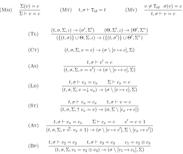
Table 3.2 shows the semantics of the rest of µ-Simd’s instructions. A tuple (t, σ, Σ, ι) denotes the execution of an instruction ι by a PE (t, σ). All the active PEs execute the same instruction at the same time. We model this phenomenon by showing, in Rule Tl, that the order in which different PEs process ι is immaterial. Thus, an instruction such as v = c causes every active PE to assign the integer c to its local variable v. We use the notation f[a 7→ b] to denote the updating of function f; that is, λx.x = a ? b : f(x). The store instruction might lead to a data-race, i.e., two PEs trying to write on the same location in the shared vector. In this case, the result is undefined due to Rule Tl. We guarantee atomic updates via v ←− va x+ 1, which reads the value at Σ(σ(vx)),

increments it by one, and stores it back. This result is also copied to σ(v), as we see in Rule At. In Rule Bp we use the symbol ⊗ to evaluate binary operations, such as addition and multiplication, using the semantics usually seen in arithmetic.

3.2. The Core Language 29 (Sp) P [pc] = stop (Θ, Σ, ∅, P, pc) → (Θ, Σ) (Bt) P [pc] = bz v, l split(Θ, v) = (∅, Θ) push(Π, ∅, pc, l) = Π0 (Θ, Σ, Π0, P, l) → (Θ0, Σ0) (Θ, Σ, Π, P, pc) → (Θ0, Σ0) (Bf) P [pc] = bz v, l split(Θ, v) = (Θ, ∅) push(Π, ∅, pc, l) = Π0 (Θ, Σ, Π0, P, pc + 1) → (Θ0, Σ0) (Θ, Σ, Π, P, pc) → (Θ0, Σ0) (Bd) P [pc] = bz v, l split(Θ, v) = (Θ0, Θn) push(Π, Θn, pc, l) = Π0 (Θ0, Σ, Π0, P, pc + 1) → (Θ0, Σ0) (Θ, Σ, Π, P, pc) → (Θ0, Σ0) (Ss) P [pc] = sync Θn6= ∅ (Θn, Σ, (pc0, Θ0, l, ∅) : Π, P, l) → (Θ0, Σ0) (Θ, Σ, (pc0, ∅, l, Θn) : Π, P, pc) → (Θ0, Σ0) (Sp) P [pc] = sync (Θn, Σ, (_, ∅, _, Θ0) : Π, P, pc + 1) → (Θ0, Σ0) (Θ0∪ Θn, Σ, Π, P, pc) → (Θ0, Σ0) (Jp) P [pc] = jump l (Θ, Σ, Π, P, l) → (Θ0, Σ0) (Θ, Σ, Π, P, pc) → (Θ0, Σ0) (It) P [pc] = ι

ι /∈ {stop, bnz, bz, sync, jump}

(Θ, Σ, ι) → (Θ0, Σ0) (Θ0, Σ0, Π, pc + 1, Θ00, Σ00) (Θ, Σ, Π, P, pc) → (Θ00, Σ00)

Table 3.4. The semantics of µ-Simd: control flow operations. For conciseness, when two hypotheses hold we use the topmost one. We do not give evaluation rules for bnz, because they are similar to those given for bz

30 Chapter 3. Divergence Analyses (Mm) Σ(v) = c Σ ` v = c (Mt) t, σ ` Tid= t (Mv) v 6= Tid σ(v) = c t, σ ` v = c (Tl) (t, σ, Σ, ι) → (σ0, Σ0) (Θ, Σ0, ι) → (Θ0, Σ”) ({(t, σ)} ∪ Θ, Σ, ι) → ({(t, σ0)} ∪ Θ0, Σ”) (Ct) (t, σ, Σ, v = c) → (σ \ [v 7→ c], Σ) (As) t, σ ` v0 = c (t, σ, Σ, v = v0) → (σ \ [v 7→ c], Σ) (Ld) t, σ ` vx= cx Σ ` cx = c (t, σ, Σ, v =↓ vx) → (σ \ [v 7→ c], Σ) (St) t, σ ` vx= cx t, σ ` v = c (t, σ, Σ, ↑ vx = v) → (σ, Σ \ [cx7→ c]) (At) t, σ ` vx= cx Σ ` cx= c c0 = c + 1 (t, σ, Σ, v←− va x+ 1) → (σ \ [v 7→ c0], Σ \ [cx7→ c0]) (Bp) t, σ ` v2 = c2 t, σ ` v3 = c3 c1= c2⊗ c3 (t, σ, Σ, v1= v2⊕ v3) → (σ \ [v17→ c1], Σ)

Table 3.5. The operational semantics of µ-Simd: data and arithmetic operations

keep the figure clean, we only show the label of the first instruction present in each basic block. This program will be executed by many threads, in lock-step; however, in this case, threads perform different amounts of work: the PE that has Tid = n will

visit n + 1 cells of the matrix. After a thread leaves the loop, it must wait for the others. Processing resumes once all of them synchronize at label l15. At this point,

each thread sees a different value stored at σ(d), which has been incremented Tid+ 1

times. Figure 3.4 (Right) illustrates divergence via a snapshot of the execution of the program seen on the left. We assume that our running program contains four threads: t0, . . . , t3. When visiting the branch at label l6 for the second time, the predicate p

is 0 for thread t0, and 1 for the other PEs. In face of this divergence, t0 is pushed

onto Π, the stack of waiting threads, while the other threads continue executing the loop. When the branch is visited a third time, a new divergence will happen, this time causing t1 to be stacked for later execution. This pattern will happen again with thread

3.3. Gated Static Single Assignment Form 31 A _µ-Simd program cfg l7: p = d % 2 bnz p, l11 l15: sync x= d − 1 ↑x= s stop l0: s = 0 d = 0 i = tid x = tid + 1 L = c × x l5: p = i − L bz p, l15 l9: x= ↓i s = s + x l11: sync d = d + 1 i = i + c jmp l5 Cycle Instruction t0 t1 t2 t3 14 l5 : p = i − L X X X X 15 l6 : bz p, l15 X X X X 16 l7 : p = d % 2 • X X X 17 l8 : bz p, l11 • X X X 18 l9 : x =↓ i • X X X 19 l10: s = s + x • X X X 20 l11: sync • X X X 21 l12: d = d + 1 • X X X 22 l13: i = i + c • X X X 23 l14: jmp l5 • X X X 24 l5 : p = i − L • X X X 25 l6 : bz p, l15 • X X X 26 l7 : p = d % 2 • • X X 27 l8 : bz p, l11 • • X X . . . 44 l5 : bz p, l15 • • • X 45 l15: sync X X X X 46 l16: x = d − 1 X X X X

Execution trace. If a thread t executes an instruction at a cycle j, we mark the entry (t, j) with the symbol _X. Otherwise, we mark it with the symbol • Figure 3.4. Execution trace of a µ-Simd program

synchronize via the sync instruction at label l15, and resume lock-step execution.

3.3

Gated Static Single Assignment Form

To better handle control dependency between program variables, we work with µ-Simd programs in Gated Static Single Assignment form (GSA, see Ottenstein et al. [1990]; Tu and Padua [1995]). Figure 3.5 shows the program in Figure 3.4 converted to GSA form. This intermediate program representation differs from the well-known Static Single Assignment proposed in Cytron et al. [1991] form because it augments φ-functions with the predicates that control them. The GSA form uses three special instructions: µ, γ and η functions, defined as follows:

• γ functions represent the joining point of different paths created by an “if-then-else" branch in the source program. The instruction v = γ(p, o1, o2) denotes

v = o1 if p, and v = o2 if ¬p;

32 Chapter 3. Divergence Analyses

l

₈

: p

₁

= d

₁

% 2

bnz p

1,

l

12

l

₁₆

: [s

₄

, d

₃

] = η[p

₀

, (s

₁

, d

₁

)]

x

₃

= d

₃

− 1

↑x

₃

= s

₄

stop

l

₀

: s

₀

= 0

d

₀

= 0

i

₀

= tid

x

₀

= tid + 1

L

₀

= c × x

₀

l

₅

:

[i

₁

,s

₁

,d

₁

]

= µ[(i

0

, s

0

,d

0

),(i

2

, s

3

, d

2

)]

p

₀

= i

1

− L

0

bz p

0

, l

16

l

₁₀

: x

₂

= ↓i

₁

s

₂

= s

₁

+ x

₂

l

₁₂

: [s

₃

] = γ(p

₁

, s

₂

, s

₁

)

d

₂

= d

₁

+ 1

i

₂

= i

₁

+ c

jmp l

5

Figure 3.5. The program from Figure 3.4 converted into GSA form

values. The instruction v = µ(o1, o2)represents the assignment v = o1 in the first

iteration of the loop, and v = o2 in the others.

• η functions represent values that leave a loop. The instruction v = η(p, o) denotes the value of o assigned in the last iteration of the loop controlled by predicate p. We use the almost linear time algorithm demonstrated by Tu and Padua [1995] to convert a program into GSA form. According to this algorithm, γ and η functions exist at the post-dominator of the branch that controls them. A label lp post-dominates

another label l if, and only if, every path from l to the end of the program goes through lp. Fung et al. [2007] shown that re-converging divergent PEs at the immediate

post-dominator of the divergent branch is nearly optimal with respect to maximizing hardware utilization. Although Fung et al. discovered situations in which it is better to do this re-convergence past lp, they are very rare. Thus, we assume that each γ or

η function encodes an implicit synchronization barrier, and omit the sync instruction from labels where any of these functions is present. These special functions are placed at the beginning of basic blocks. We use Appel’s parallel copy semantics (see Appel [1998]) to evaluate these functions, and we denote these parallel copies using Hack’s

3.4. The Simple Divergence Analysis 33

matrix notation described in Hack and Goos [2006]. For instance, the µ assignment at l5, in Figure 3.5 denotes two parallel copies: either we perform [i1, s1, d1] = (i0, s0, d0),

in case we are entering the loop for the first time, or we do [i1, s1, d1] = (i2, s3, d2)

otherwise.

We work on GSA-form programs because this intermediate representation allows us to transform control dependency into data dependency when calculating uniform variables. Given a program P , a variable v ∈ P is data dependent on a variable u ∈ P if either P contains some assignment instruction P [l] that defines v and uses u, or v is data dependent on some variable w that is data dependent on u. For instance, the instruction p0 = i1− L0 in Figure 3.5 causes p0 to be data dependent on i1 and L0. On the other

hand, a variable v is control dependent on u if u controls a branch whose outcome determines the value of v. For instance, in Figure 3.4, s is assigned at l10 if, and

only if, the branch at l8 is taken. This last event depends on the predicate p; hence,

we say that s is control dependent on p. In the GSA-form program of Figure 3.5, we have that variable s has been replaced by several new variables si, 0 ≤ i ≤ 4.

We model the old control dependence from s to p by the γ assignment at l12. The

instruction [s3] = γ(p1, s2, s1) tells that s3 is data dependent on s1, s2 and p1, the

predicate controlling the branch at l9.

3.4

The Simple Divergence Analysis

The simple divergence analysis reports if a variable v is uniform or divergent. We say that a variable is uniform if, at compile time, it is know that all threads will see the same value for this variable at run-time. A uniform variable meets the condition in Definition 2. If, at compile time, it is not possible to define if the values seen by all threads for a variable are the same, this variable is called a divergent variable. For example, loading data from different memory positions into a same variable name might not cause a data divergence, but that is not possible to define at compile time. In cases like this the analysis is conservative and classifies these variables as divergent. In order to find statically a conservative approximation of the set of uniform variables in a program we solve the constraint system in Figure 3.6. In Figure 3.6 we letJvK denote the abstract state associated to variable v. This abstract state can be an element of the lattice > < U < D. This lattice is equipped with a meet operator ∧, such that a ∧ a = a, a ∧ > = > ∧ a = a, a ∈ {U, D}, and U ∧ D = D ∧ U = D. In Figure 3.6 we use o1⊕ o2 for any binary operator, including addition and multiplication. Similarly,

34 Chapter 3. Divergence Analyses

v = c × Tid [TidD] JvK = D v = ⊕o [AsgD] JvK = JoK v←− va _x+ c [AtmD] JvK = D v = c [CntD] JvK = U v = γ[p, o1, o2] [GamD] JpK = U JvK = Jo1K ∧ Jo2K v = η[p, o] [EtaD] JpK = U JvK = JoK v = o1⊕ o2 [GbzD] JvK = Jo1K ∧ Jo2K v = γ[p, o1, o2] or v = η[p, o] [PdvD] JpK = D JvK = D v = µ[o1, . . . , on] [RmuD] JvK = Jo1K ∧ Jo2K ∧ . . . ∧ JonK

Figure 3.6. Constraint system used to solve the simple divergence analysis

Definition 2 (Uniform variable). A variable v ∈ P is uniform if, and only if, for any state (Θ, Σ, Π, P, pc), and any σi, σj ∈ Θ, we have that i, σi ` v = c and j, σj ` v = c.

Sparse Implementation. If we see the inference rules in Figure 3.6 as transfer func-tions, then we can bind them directly to the nodes of the source program’s dependence graph. Furthermore, none of these transfer functions is an identity function, as a quick inspection of the rules in Figure 3.8 reveals. Therefore, our analysis admits a sparse implementation, as defined by Choi et al. Choi et al. [1991]. In the words of Choi et al., sparse data-flow analyses are convenient in terms of space and time because (i) useless information is not represented, and (ii) information is forwarded directly to where it is needed. Because the lattice used in Figure 3.6 has height two, that constraint system can be solved in two iterations of a unification-based algorithm. Moreover, if we ini-tialize every variable’s abstract state to U, then the analysis admits a straightforward solution based on graph reachability. As we see from the constraints, a variable v is divergent if either it (i) is assigned a factor of Tid, as in Rule TidD; or (ii) it is defined

by an atomic instruction, as in Rule AtmD; or (iii) it is the left-hand side of an instruc-tion that uses a divergent variable. From this observainstruc-tion, we let a data dependence graph Gthat represents a program P be defined as follows: for each variable v ∈ P , let nv be a vertex of G, and if P contains an instruction that defines variable v, and uses

variable u, then we add an edge from nu to nv. To find the divergent variables of P , we

start from ntid, plus the nodes that represent variables defined by atomic instructions,

3.4. The Simple Divergence Analysis 35 d₀ d1 d2 µ + η d3 p0 L₀ i1 − c x0 tid + i₀ i₂ 0 × µ + 1 p1

Figure 3.7. The dependence graph created for the program in Figure 3.5. We only show the program slice (Weiser [1981]) that creates variables p1 and d3.

Divergent variables are colored gray.

Moving on with our example, Figure 3.7 shows the data dependence graph created for the program in Figure 3.5. Surprisingly, we notice that the instruction bnz p1, l12

cannot cause a divergence, even though the predicate p1 is data dependent on variable

d1, which is created inside a divergent loop. Indeed, variable d1 is not divergent,

although the variable p0 that controls the loop is. We prove the non-divergence of d1

by induction on the number of loop iterations. In the first iteration, every thread sees d1 = d0 = 0. In subsequent iterations we have that d1 = d2. Assuming that at the n-th

iteration every thread still in the loop sees the same value of d1, then, the assignment

d2 = d1+ 1 concludes the induction step. Nevertheless, variable d is divergent outside

the loop. In this case, we have that d is renamed to d3 by the η-function at l16. This

η-function is data-dependent on p0, which is divergent. That is, once the PEs synchronize

at l16, they might have re-defined d1 a different number of times. Although this fact

cannot cause a divergence inside the loop, divergence might still happen outside it. Theorem 1. Let P be a µ-Simd program, and v ∈ P . If JvK = U , then v is uniform.

Proof. The proof is a structural induction on the constraint rules used to derive JvK = U :