Budget Processes: Theory and Experimental Evidence

(1)

Montréal Octobre 1999

Série Scientifique

Scientific Series

99s-33

Budget Processes: Theory and

Experimental Evidence

Karl-Martin Ehrhart, Roy Gardner,

(2)

CIRANO

Le CIRANO est un organisme sans but lucratif constitué en vertu de la Loi des compagnies du Québec. Le financement de son infrastructure et de ses activités de recherche provient des cotisations de ses organisations-membres, d=une subvention d=infrastructure du ministère de la Recherche, de la Science et de la Technologie, de même que des subventions et mandats obtenus par ses équipes de recherche.

CIRANO is a private non-profit organization incorporated under the Québec Companies Act. Its infrastructure and research activities are funded through fees paid by member organizations, an infrastructure grant from the Ministère de la Recherche, de la Science et de la Technologie, and grants and research mandates obtained by its research teams.

Les organisations-partenaires / The Partner Organizations

$École des Hautes Études Commerciales $École Polytechnique

$Université Concordia $Université de Montréal

$Université du Québec à Montréal $Université Laval

$Université McGill $MEQ

$MRST

$Alcan Aluminium Ltée $Banque Nationale du Canada $Bell Québec

$Développement des ressources humaines Canada (DRHC) $Egis

$Fédération des caisses populaires Desjardins de Montréal et de l=Ouest-du-Québec $Hydro-Québec

$Imasco

$Industrie Canada $Microcell Labs inc.

$Raymond Chabot Grant Thornton $Téléglobe Canada

$Ville de Montréal

Reproduction partielle permise avec citation du document source, incluant la notice ©.

Short sections may be quoted without explicit permission, provided that full credit, including © notice, is given to the source.

ISSN 1198-8177

Ce document est publié dans l=intention de rendre accessibles les résultats préliminaires de la recherche effectuée au CIRANO, afin de susciter des échanges et des suggestions. Les idées et les opinions émises sont sous l=unique responsabilité des auteurs, et ne représentent pas nécessairement les positions du CIRANO ou de ses partenaires.

This paper presents preliminary research carried out at CIRANO and aims at encouraging discussion and comment. The observations and viewpoints expressed are the sole responsibility of the authors. They do not necessarily represent positions of CIRANO or its partners.

(3)

Budget Processes: Theory and Experimental Evidence

*

Karl-Martin Ehrhart

H

, Roy Gardner

I

, Jürgen von Hagen

'

, Claudia Keser

&

Résumé / Abstract

Ce texte étudie des processus de construction budgétaire, tant d'un point de vue théorique que d'un point de vue de leur application expérimentale. Nous spécifions une condition suffisante afin que l’équilibre électoral soit le même pour les processus de construction budgétaire qu'ils soient de type « top-down » (par le haut) ou de type « bottom-up » (par le bas). D'autre part, et bien que cela soit souvent supposé, il n'est pas toujours vrai qu'à l’équilibre électoral un processus de construction budgétaire « top-down » conduise à un plus faible budget global que ne le ferait un processus budgétaire de type « bottom-up ». Pour tester les conséquences de la théorie de l’équilibre électoral sur les processus de construction budgétaire, une série de 128 expériences a été conduite en laboratoire. Les résultats de ces expériences sont largement conformes à la théorie de l’équilibre électoral, aussi bien au niveau des donnés agrégés qu'au niveau des résultats individuels. Plus particulièrement, l'étude des résultats révèle que les joueurs font preuve d'une véritable rationalité de décision tant pour formuler leur proposition que pour établir leur stratégie de vote. Enfin, une information plus complète et moins de catégories de dépenses conduisent à un plus grand succès de prévision de la théorie de l’équilibre électoral et réduisent le temps nécessaire pour atteindre une ratification budgétaire.

This paper studies budget processes, both theoretically and experimentally. We give a sufficient condition for top-down and bottom-up budget processes to have the same voting equilibrium. Furthermore, at a voting equilibrium, it is not always true, as often presumed, that a top-down budget process leads to a smaller overall budget than does a bottom-up budget process. To test the implications for budget processes of voting equilibrium theory, we conduct a series of 128 voting experiments using subjects in a behavior laboratory. The experimental evidence from these experiments is well organized by voting equilibrium theory, both at the aggregate level and at the individual subject level. In particular, subjects display considerable evidence of rationality in their proposals and votes. More complete information and fewer spending

*

Corresponding Author : Claudia Keser, CIRANO, 2020 rue University, 25ème étage, Montréal, Qc, Canada

H3A 2A5 Tél. : (514) 985-4000 Fax : (514) 985-4039 courriel : keserc@cirano.umontreal.ca

†

University of Karlsruhe

‡_{Indiana University and ZEI, University of Bonn} §

University of Bonn, Indiana University, and CEPR ¶_{University of Karlsruhe and CIRANO}

(4)

categories lead to greater predictive success of voting equilibrium theory, and reduce the time needed to reach a budget decision.

Mots Clés : Processus de construction budgétaire, équilibre électoral, économie expérimentale

(5)

1. Introduction

A budget process is a system of rules governing the decision making that leads to a budget, from its formulation, through its legislative approval, to its execution. Consider the budget process of the United States government. The President formulates a budget proposal as part of his annual obligation to report on the State of the Union. Each house of Congress then reworks the budget proposal, with a final budget being passed by both houses for presidential approval.

In the last quarter century, the details of the budget process, both in the United States and in other countries, have been the object of considerable research (Wildavsky, 1975; Ferejohn and Krehbiel, 1987; Alesina and Perotti, 1995, 1999; von Hagen and Harden, 1995, 1996; see also the contributions in Poterba and von Hagen, 1999). There is a growing body of empirical research, based on international comparative studies, suggesting that the design of budget processes has considerable influence on the fiscal performance of governments. This has also been reflected in political decisions. In the United States, the Budget Act of 1974, the Gramm-Rudman-Hollings Act of 1985, and the Budget Enforcement Act of 1991 all tried to reduce excessive government spending and deficits by changes in the budget process. In the European Union, the Maastricht Treaty on European Union of 1992 mandates reform of budget processes of the member states to enhance fiscal discipline.

One aspect of the budget process that has received considerable attention is the sequence of budgeting decisions. Traditionally, Congress votes on budget items line-by-line, or category-by-category. The sum of all spending approved by Congress emerged as the overall budget—a budget process called bottom-up. The budget reforms stemming from the Budget Act of 1974 replaced this tradition with a different sequence. First, Congress was to vote on the total size of the budget. Once that was determined, Congress would allocate that total budget among spending categories. A budget process of that type is called a top-down process. It was argued at the time, that a top-down budget process would lead to a better outcome, in particular, to a smaller budget, than would a bottom-up budget process (Committee on the Budget, 1987).

A similar presumption is shared by many international organizations, which act as if a top-down budget process is inherently preferable to a bottom-up process. The Organization of Economic Cooperation and Development (OECD, 1987) reported approvingly that several countries adopted top-down budget processes in quest of greater fiscal discipline. Schick (1986) analyzes this report, explaining (and supporting) the thinking behind it in great detail. The International Monetary Fund (IMF) expresses a similar preference for top-down processes (IMF, 1996).

The presumption in favor of top-down budgeting stands in stark contrast to voting equilibrium theory. Suppose rational agents participate as voters in a budget process. In particular, if voters are sophisticated in the sense of Farquharson (1969) and Kramer (1972): they consider the implications of voting in early stages of the budget process for later stages of the process. Furthermore, assume that voters have convex preferences over the individual dimensions of the budget, and that the budget process divides the decision-making process into a sequence of

(6)

one-dimensional decisions. Based on these assumptions, Ferejohn and Krehbiel (1987) show that the voting equilibrium of a top-down budget process generally differs from the equilibrium of a bottom-up process: sequence matters. However, there is no unambiguous relation between sequence and the size of the budget. Depending on the voters’ preferences, a top-down process can lead to larger or smaller budgets.

This argument, based on voting equilibrium, depends crucially on the rationality of voters—itself an empirical issue. One way to get at this empirical issue is with controlled laboratory experiments. While laboratory experiments create artificial environments, they have the advantage over international comparisons that the design of an institution and the setting of a decision-making process can be controlled much more precisely. Previous experiments have found some evidence for sophisticated voting in two stage voting games (Holt and Eckel, 1989; Davis and Holt,1993). Similarly, in a pilot experiment Gardner and von Hagen (1997) find that structurally induced voting equilibrium best accounts for the data from their experimental trials of bottom-up and top-down budget processes.

This paper reports on a series of 128 independent trials of voting over budgets. The first testable implication of the theory of structurally induced voting equilibrium is that the outcome of a budget process depends on the voters’ preferences and on structure of the process. Therefore, we vary voters’ preferences and the structure of the process (bottom-up or top-down) in a systematic way over these 128 trials. The second testable implication of the theory concerns the effect dimensionalitythe number of spending categorieshas on the budget process and its outcome. Whereas previous experiments have been confined to two dimensions, ours include treatments with two and four dimensions. This leads to a gain in applicability, since naturally occurring budget processes only rarely deal with two dimensions. A third testable implication of the theory concerns the effect of incomplete information on the budget process and its outcome. Whereas previous experiments have assumed complete information (each voter knows the preferences of all voters), ours include treatments with complete and incomplete information. In the incomplete information treatment, a voter knows only his or her own preferences, and not the preferences of any other voter. This extension is again made in the interest of realism. Many budgets are processed in situations where a voter has limited knowledge of the preferences of other voters.

Our main result is that institutions matter. The data from all treatments correspond closely to the theory of voting equilibrium, and institutions drive those equilibria. The subjects display a high degree of sophistication over all treatments. Both extra dimensionality and incomplete information increase the complexity of the decision problem subjects face, and increase the number of periods needed to reach a final decision.

The paper is organized as follows. The next section sets out the general model, as well as the specification we have implemented experimentally. Section 3 describes the experimental design, as carried out at the economics behavior laboratory of the University of Karlsruhe. Our aggregate results are presented in section 4; individual results, in section 5. Section 6 concludes with the policy implications of these experiments.

(7)

2. A model of budgeting

We present a model of budgeting which is an extension to many dimensions of the model of Ferejohn and Krehbiel (1987). To solve this model, we use the notion of structurally induced equilibria following McKelvy (1979).

2.1 The general model

There are n voters, indexed by i, i=1,..., n. Using majority rule, the voters decide on the size and allocation of a budget. There are m spending categories in the overall budget. Let Rm+ denote the non-negative orthant of m-dimensional Euclidean space, the space of all possible budget vectors. Let the vector x = (x1, ..., xn) ∈ Rm+ denote a possible budget, where xj represents spending in the budget category j. The total spending implied by the budget vector x is

B = x_j

j=1 m

∑

.

Each voter i has preferences over budgets x represented by his or her utility function ui(x). We assume that each voter i has an ideal budget (or an ideal point) x*(i). The closer the actual budget is to a player’s ideal budget the higher is the player’s utility, where closeness is measured by the Euclidean distance function. This implies

u_i( )x = − [ − *( )] =

∑

K_i x_j x i_j j m 2 1 ,

where Ki is the utility attached to the ideal point.1 In general, each voter i has an ideal point x*(i) distinct from that of all other voters.

Several interpretations of players and their ideal points are possible. For instance, the players may be spending ministers in a coalition government. In this case, an ideal point represents the overall spending budget a spending minister would like to see enacted. Again, suppose the player is a member of a legislature. Then the ideal point may represent a commitment made by that legislator during his or her successful election campaign, to see that the ideal point (or something as close to it as possible ) is enacted into legislation.

Assume that decisions are made by majority rule, applied in a pairwise fashion over two budget proposals x and y. If the number of those voting for x is greater than the number of those voting for y, x defeats y. A budget x is a voting equilibrium, or a Condorcet equilibrium, if it defeats all other budgets. Note that for n ≥ 3 and m ≥ 2, the paradox of voting—non-existence of a Condorcet equilibrium—can occur ( Riker 1962).

1_{In the two dimensional case the Euclidean utility function leads to circular indifference curves. More} general preferences are studied experimentally in Lao-Araya (1998), whose results suggest that voting equilibrium theory is robust with regard to elleptical indifference curves.

(8)

To address the problem posed by the nonexistence of voting equilibrium in many dimensions, various institutions have evolved, which use majority rule for a single dimension at a time. With Euclidean preferences, there exists a voting equilibrium in each dimension, identified with the median voter in that dimension. With m budget categories, at most m such decisions are required, one for each spending category. The structure of a budget process induces a voting equilibrium. The voting equilibrium so induced depends on the process. With an odd number of voters, each with a unique ideal point, the voting equilibrium is unique.

In a bottom-up budget process the sequence of votes is taken in each dimension at a time. For instance, if there are two dimensions the vote is taken first on one dimension and then on the other. With Euclidean preferences in two dimensions, the voting equilibrium is invariant under permutations of the sequence of dimensions. One gets the same bottom-up equilibrium if the vote on dimension 1 is first, or if the vote on dimension 2 is first. This also holds true for higher dimensions, when m ≥ 2. The structurally induced equilibrium is constructed from the voting equilibrium in each dimension of the process. Let xbu denote the equilibrium induced by a

bottom-up budget process.

In a top-down budget process, the sequence of votes starts with a vote on the total budget. Then votes are taken on the distribution of total spending over m-1 spending categories. For instance, if there are two dimensions, the vote is taken first on the total budget and then on a dimension orthogonal to that one, the dimension corresponding to the difference in the two spending categories.2Again, the voting equilibrium is invariant under permutations of the sequence of orthogonal dimensions. The structurally induced equilibrium is constructed from the the voting equilibrium in each dimension of the voting taken. Let xtd denote the equilibrium

induced by a top-down budget process.

In general, xtd does not equal xbu. A sufficient condition for xtd and xbu to be equal is that there exist a Condorcet equilibrium xC over the entire space of budgets, in which case xtd and xbu equal xC. As already pointed out, this condition is unlikely to be satisfied in practice. One way to see this in two dimensions (the same insight holds for higher dimensions) is to note that a Condorcet equilibrium must have majority support in every dimension. Consider the case of bottom-up voting first. We seek possible configurations under which a median voter is the same in both dimensionshence this median voter’s ideal point is the Condorcet equilibrium. The simplest such configuration is if all the voters’ ideal points are arrayed on a straight line (see Figure 1). The first vote is determined by the median of the ideal points projected onto the first budget dimension (line a) and the second vote by the median of the ideal points projected onto the second dimension (line b). Line a and line b meet at the bottom-up equilibrium xbu which is equal to the ideal point x*(2) and therefore equal to the desired Condorcet equilibrium xC.

Next consider the case of top-down voting. The first vote is determined by the median of the preferred total budgets. This decision is graphically represented by the median -45° line through the ideal points (line c). The second decision, the vote on the first category, is graphically

2

This vote could also be taken over a non-orthogonal dimension, such as dimension 1 or dimension 2, without changing the resulting voting equilibrium.

(9)

represented by the median 45° line through the ideal points (line d). Line c and line d also meet at

x*(2). Thus, xtd equals xC as well.

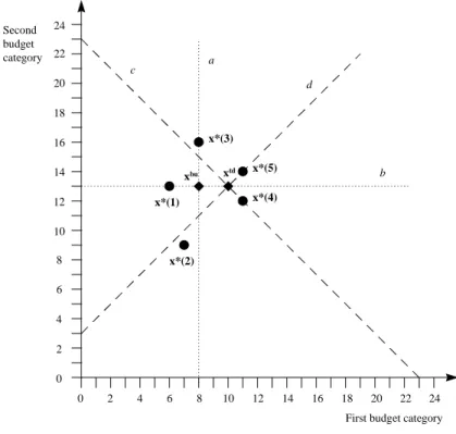
When this sufficient condition is not satisfied, , bottom-up and top-down voting may lead to different outcomes. See figures 2 and 3, which illustrate this for the case of n = 5, m = 2.

Second budget category

First budget category

x*(2) = xbu_{= x}td _{= x}C x*(1) x*(3) a b d c

Figure 1: Condorcet equilibrium

2.2 Specific models

For all experiments studied here, the number of voters, n, equals 5. The number of spending categories, m, equals either 2 or 4. To specify the voters' utility functions, we have two designsone design is such that the voting equilibrium of a top-down budget process leads to a larger budget than the voting equilibrium of a bottom-up budget process, and vice versa in the other design.

We discuss first the simpler case m = 2. To specify the voters' utility functions, we have two designs, design I and design II. They are presented in Table 1. Notice that the two designs differ by voter 4’s ideal point only. Voters 1, 2, 3, and 5 have the same ideal points in both designs. The general intention behind these two designs is to make the difference between the equilibrium induced by a bottom-up process, xtd , and the equilibrium induced by a top-down process, xbu, large and in different directions. As can be seen in Table 2, in design I, the total budget corresponding to xbu is smaller than the total budget corresponding to xtd , while the opposite is true in design II.

(10)

For design I, the median of the dimension 1 components of the ideal points is 8. The median of the dimension 2 components of ideal points is 13. Putting the components from the two dimensions together, we get (8, 13). The solution induced by the bottom-up process is the vector (8, 13). This is xbu. The total spending under this budget is 21.

The solution induced by the top-down process is the vector (10, 13). This is xtd. The total spending under this budget is 23. To find the top-down solution, start with two orthogonal dimensions, corresponding to the x1+x2 dimension and the x1-x2 dimension. In the x1+x2 dimension, the sum of ideal points components of the five players is 19, 16, 24, 23, and 25, respectively. The median of these components is 23. In the x1-x2 dimension, the difference of ideal points components of the five players is -7, -2, -8, -1, -3, respectively. The median of these components is -3. Solving the pair of equations x1+x2 = 23 and x1-x2= -3 yields x1 = 10, x2 = 13.

The ideal points and the voting equilibria of design I are shown in Figure 2. Graphically, the bottom-up equilibrium xbu = (8,13) is determined by the intersection of the vertical median line through the ideal points a and the horizontal median line b. The top-down equilibrium xtd = (10,13) is determined by the intersection of the -45° median line c and the 45° median line d. Notice that xtd is different from xbu. Bottom-up voting leads to a smaller budget, 21, than does top-down voting, 23.

For design II, the solution xbu induced by the bottom-up process is the vector (8, 13). The total spending under this budget is 21. This is the same as in design I. However, for the top down process, the solution xtd is the vector (8, 11). The total spending under this budget is 19. Notice that xtd is different from xbu, but in contrast to design I, top-down voting leads to a smaller budget, 19, than does bottom-down voting, 21 (see Figure 3). This is because the median voter, here voter 4, goes from wanting to spend 23 units in design I to 18 units in design II.

We consider now the case m = 4. The basic principle in getting from two dimensions to four dimensions is projection: (x1, x2) maps into (x1, x2, x1, x2). The ideal points of each player are presented in Table 1. The medians of the ideal points in each dimension are preserved under projection.

For design III, which is the projection of design I, the medians in dimensions 1 and 3 are 8; in dimensions 2 and 4, 13. Putting the components from the four dimensions together, we get

xbu , the vector (8, 13, 8, 13). The total spending under this budget is 42.

The solution xtd induced by the top-down process is the vector (10, 13, 10, 13); this again follows by projection. The total spending under this budget is 46. Notice that xtd is different from

xbu, and in particular that xtd spends more than xbu, 46 versus 42.

For design IV, which is the projection of design II, the medians in dimensions 1 and 3 of the ideal points are 8; in dimensions 2 and 4, 13. Putting the components from the four dimensions together, we get (8, 13, 8, 13) as the bottom-up vector xbu . Total spending under this budget is 42.

(11)

The solution xtd induced by the top-down process is the (8, 11, 8, 11). The total spending under this budget is 38. Notice that xtd also differs from xbu. In contrast to design III, top-down voting leads to a smaller budget, 38, than the budget of size 42 that bottom-up voting adopts.

Table 1: Individual ideal points and utility function, x*(i) and ui(x)

m = 2 m = 4

Design I Design II Design III Design IV

Voter i x1*(i) x2*(i) x1*(i) x2*(i) x1*(i) x2*(i) x3*(i) x4*(i) x1*(i) x2*(i) x3*(i) x4*(i) 1 2 3 4 5 6 7 8 11 11 13 9 16 12 14 6 7 8 9 11 13 9 16 9 14 6 7 8 11 11 13 9 16 12 14 6 7 8 11 11 13 9 16 12 14 6 7 8 9 11 13 9 16 9 14 6 7 8 9 11 13 9 16 9 14 Utility Function Of voter i ui(x) 15 2 1 2 − − =

∑

[x_j x i*_j( )] j 30 2 1 4 − − =

∑

[x_j x i*_j( )] j

Table 2: Voting equilibria

m = 2 m = 4

Design I Design II Design III Design IV

Process x1 x2 x1 x2 x1 x2 x3 x4 x1 x2 x3 x4

Bottom-up 8 13 8 13 8 13 8 13 8 13 8 13

Σ 21 21 42 42

Top-down 10 13 8 11 10 13 10 13 8 11 8 11

(12)

2 4 6 8 0 10 12 14 16 18 20 22 24 0 2 4 6 8 10 12 14 16 18 20 22 24 xbu xtd x*(3) x*(5) x*(4) x*(1) x*(2) a b c d Second budget category

Figure 2: Voting equilibria (design I)

Second budget category 2 4 6 8 0 10 12 14 16 18 20 22 24 0 2 4 6 8 10 12 14 16 18 20 22 24 xbu xtd x*(3) x*(5) x*(4) x*(1) x*(2) a b c d

(13)

3. Experimental design

The instructions for the experiment are based on those of the classic voting experiment conducted by Plott and Krehbiel (1979). Copies of the instructions (in German) are available from the authors upon request.

In the experiment, subjects are told that each of them is member of a group of 5 subjects. In designs I and II, the group’s task is to decide on how many integer-valued tokens to spend on two activities, called A and B. In the instructions for a bottom-up budget process, subjects are told that they first have to decide on the number of tokens to be spent on activity A. Their decision on this number is final. They then have to decide on the number of tokens to be spent on activity B, at which point they have completed their task. In the instructions for a top-down budget process, subjects are told that they first have to decide on the number of tokens to be spent on activities A and B together. Their decision on this number is final. They then have to decide on the number of tokens to be spent on activity A, at which point they have completed their task.

In designs III and IV, the group’s task is to decide on how many tokens to spend on four activities, called A, B, C, and D. In the instructions for a bottom-up budget process, subjects are told that they first have to decide on the number of tokens to be spent for activity A. Their decision on this number is final. They then repeat this process for activities B, C, and D in that order, at which point they have completed their task. In the instructions for a top-down budget process, subjects are told that they first have to decide on the number of tokens to be spent on activities A, B, C, and D together. Their decision on this number is final. They then have to decide on the number of tokens to be spent on activities, A, B, and C in that order, at which point they have completed their task.

At each step, the decision task is to decide on a number of tokens to be spent on some category or combination of categories. The decision process starts with a proposal on the floor which equals zero. At any point in time, each subject has the right to propose an amendment. If an amendment is proposed, then the group has to vote on it. If the proposed amendment is accepted, then it becomes the new proposal on the floor. If the proposed amendment is rejected, it has no effect; the proposal on the floor remains unchanged. In that case, each subject is free to propose another amendments, but only one amendment, at a time. At any point of time, a subject may also propose to end the process. If this proposal is accepted, then the proposal on the floor is considered accepted. If the proposal to end deliberations is rejected, then new amendments may be proposed or new proposals for ending the process may be made.

All votes are based on simple majority rule. This implies that if three or more members of the group vote in favor of the proposal, then it wins. Otherwise the proposal is rejected.

In the beginning of the experiment, each subject is informed about his personal payoff (or utility) function. The instructions give each subject the exact formula for the payoff function, which is also explained to him. In the case of two spending categories (design I and design II), the subject is given a table which shows his or her payoff for each combination of numbers in the two spending categories. In all four designs, each subject can, in the final dimension of voting, call up

(14)

on his or her computer screen to see individual payoff for the proposal on the table and the proposed amendment.

Besides designs I through IV, which differ with respect to the number of spending categories and the ideal points, we distinguish between two informational treatments. In the complete information treatment each subject knows not only his own ideal point, but also the ideal points of the four other players in his group. In the incomplete information treatment, each player is only informed about his own ideal point.

The experiments were organized at the University of Karlsruhe. Subjects were students from various disciplines. The experiments were computerized. Each subject was seated at a computer terminal which was isolated from other subjects’ terminals by wooden screens. The subjects received written instructions which were also read aloud by a research assistant. Before an experiment started, each subject had to answer at his computer terminal a short questionnaire (10 questions) concerning the instructions. Only after all subjects had given the right answers to all questions did decision-making begin. No communication other than through the recognition of proposals and the announcement of the outcomes of votes was permitted.

We organized sessions with 15 or more subjects. Thus, no subject could identify with which of the other participants he or she was grouped. Each subject participated in exactly one experiment; thus, each group of 5 subjects yielded an independent observation. For each design (4), each budget process (2), and each information condition (2), we obtained 8 independent observations, for a total of 128 experiments. Table 3 gives an overview of the experimental design. In obtaining these 128 independent observations, we also acquired data on 640 subjects, 5 each per experiment.

Table 3: Treatment design

Number of groups (subjects)

M = 2 m = 4

Design I Design II Design III Design IV Complete information Bottom-up Top-down 8 (40) 8 (40) 8 (40) 8 (40) 8 (40) 8 (40) 8 (40) 8 (40) Incomplete information Bottom-up Top-down 8 (40) 8 (40) 8 (40) 8 (40) 8 (40) 8 (40) 8 (40) 8 (40)

(15)

4. Experimental results

This section considers aggregate data from the experiment; the next section, individual data. Start with the sizes of the overall budgets we observe in these 128 experiments. Tables 4 (for the 2-dimensional treatment) and 5 (for the four-dimensional treatment) give an overview of observed group voting outcomes in all treatments. In situations where top-down voting equilibria spend more than bottom-up voting equilibria (designs I and III), we observe this very clearly in the data. The same holds true in situations where top-down voting equilibria spend less than bottom-up voting equilibria (designs II and IV). With complete information, the differences between bottom-up and top-down total budgets are significant at the 10% level in design I, and at the 5 percent level in designs II, III and IV (Mann-Whitney U-test). With incomplete information, the corresponding differences are significant at the 10 percent level in design II, and at the 5 percent level in designs III and IV. In design I the difference is not statistically significant at the 10 percent level; but it does go in the right direction.3

Result 1. Sequence matters. The outcomes observed under bottom-up and top-down voting differ from each other significantly.

We next show that voting equilibrium is a good predictor. To see this visually, first pool the data from designs I and II, and call the pooled data the 2-dimensional treatment. Figure 4 shows the scatter diagram of 2-dimensional treatment data relative to the predicted value. Notice how tight the scatter is around the voting equilibrium prediction; the average Euclidean distance of an observation from the predicted value is 1.5, a small number relative to a predicted total sum of between 19 and 23. A similar picture emerges for the 4-dimensional treatment, where the average Euclidean distance of an observation from the predicted value is 2.6, again a small number relative to a predicted total sum of between 38 and 46. Pooling over all 128 observations, the average Euclidean distance of the observed budgets from voting equilibrium is 2.1.

Result 2. Voting equilibrium is a good predictor of budget outcome. The average distance of observed outcomes from predicted equilibrium is 2.1, a small number.

(16)

Table 4: Average budgets in the two-dimensional treatments

Design I Design II

Information Bottom-up Top-down Bottom-up Top-down

Complete Incomplete 21.4 22.6 22.5 22.6 21.4 21.5 19.0 20.1 Voting equilibrium 21 23 21 19

Table 5: Average budgets in the four-dimensional treatments

Design III Design IV

Information Bottom-up Top-down Bottom-up Top-down

Complete Incomplete 42.1 43.4 46.4 46.6 43.0 43.8 38.0 38.6 Voting equilibrium 42 46 42 38

Next, introduce another measure of closeness of an observed budget to a predicted equilibrium: an observation is close to predicted equilibrium if it does not deviate from it by more than one unit in any spending category. Over all treatments, 53.9% are close (10 out of 128 outcomes, or 7.8%, hit the predicted equilibrium exactly).

Table 6 reports the percentages of observations close to the voting equilibrium prediction for all information-dimensionality treatments. First, we see that with complete information, a higher percentage of outcomes is equal or close to the voting equilibrium than under incomplete information. This is true for each dimensional treatment separately, as well as on average, the respective averages being 62.5% versus 45.3%. Second, we see that with lower dimensionality, a higher percentage of outcomes is equal or close to the voting equilibrium than with higher dimensionality. This is true for each information treatment separately, as well as on average, the respective averages being 67.2% versus 40.6%.

Result 3. Institutions matter: more than half (53.9%) of all observed budgets are close to the predicted voting equilibrium.

(17)

Figure 4: Distribution of outcomes around equilibrium

It is mathematically easier to realize an outcome which is equal or close to the voting equilibrium in two dimensions than in four dimensions. To address this concern, we apply to the data in Table 6 Selten’s (1991) measure of predictive success, which adjusts for dimensionality in the following way. Define the hit rate as the frequency of outcomes close to the voting equilibrium; define the area rate as the area of all points near the voting equilibrium, relative to the set of reasonable outcomes—outcomes any reasonable theory might allow for. Selten’s measure then is the difference between the hit rate and the area rate. In particular, the area rate in two dimensions is greater than the area rate in four dimensions.

To see this, consider the set of natural numbers bounded in each direction by the minimum and the maximum values of subjects’ ideal points. Call this the set of reasonable

outcomes—it contains the set of Pareto optima, and also includes outcomes which are nearly

Pareto optima. In designs I and II (dimension 2), the set of reasonable outcomes is the rectangle defined by the corners (6,9), (6,16), (11,9), (11,16), and contains 48 points. The area close to the voting equilibrium covers 9 points, so the area rate is 9/48 or 19 percent.

In designs III and IV (dimension 4), the set of reasonable outcomes is the polyhedron defined by the points (6,9,6,9), (6,16,6,16), (11,16,11,16), and (11,9,11,9), and contains 2304 points. The area equal or close to the voting equilibrium covers 81 points, so the area rate is 81/2304 or 3%. This verifies mathematically that it is harder to get close to a voting equilibrium in four dimensions where the area rate is 3%, than in two dimensions, where the area rate is 19%.

-4 -3 _-2 -1 0 ₁ 2 ₃ 4 -4 -3 0 2 4 0 2 4 6 8 1 0 1 2 1 4 F requ ency

F irst bu dget catego ry

Seco nd bu dget catego ry

(18)

Table 6: Percentage of budgets close to the voting equilibrium budget

Information Two-dimensional Four-dimensional Average

Complete 78.1 46.9 62.5

Incomplete 56.3 34.4 45.3

Average 67.2 40.6 53.8

Given these area rates, we can compute the measures of predictive success for the dimensionality treatment; Table 7 shows the results. In two dimensions, the hit rate is 67.2% and the area rate is 19%, yielding a predictive success of 48.2%. In four dimensions, the hit rate is 40.6% and the area rate is 3%, yielding a predictive success of 37.6%. Although predictive success is still greater in two dimensions than in four, the difference is much reduced. To put these levels of predictive success in context, note that the predictive success of Nash equilibrium theory is often less than 5% (Keser and Gardner, 1999).

Result 4. The predictive success of voting equilibrium theory is 43%. Predictive success increases with complete information, and with fewer spending categories.

Table 7: Predictive Success of Voting Equilibria

Information Two-dimensional Four-dimensional Average

Complete 59.1 43.9 51.5

Incomplete 37.3 31.4 34.4

Average 48.2 37.6 43.0

Table 8 shows the average number of moves—a proposal followed by a vote—needed to reach a budget decision in the information-dimensionality treatments. To reach a budget decision takes about 30 percent more moves with incomplete information, as opposed to complete information. To reach a budget decision in four dimensions takes about twice as many moves as in two dimensions. Since the 4-dimensional case requires twice as many final decisions made as the 2-dimensional case, we conclude that, relative to the number of spending categories the same effort is needed to reach a budget decision in both cases.

(19)

Result 5. The number of moves needed to reach a budget decision is greater with incomplete information than with complete information. The number of moves needed to reach a budget decision increases proportionally with the number of spending categories.

Table 8: Average number of moves to reach the budget decision

Information Two-dimensional Four-dimensional

Complete Incomplete 11.0 14.5 22.6 28.8 5. Individual behavior

Now turn to data on individual behavior. We consider first the effect of the information treatment on individual proposals. In two dimensions with incomplete information, subjects propose their ideal points 55.9% of the time; with complete information, 42.5%. This difference is significant at the 1 percent level (χ2 - test). In four dimensions with incomplete information, subjects propose their ideal points 47.8% of the time; with complete information, 40.8%. This difference is significant at the 5 percent level (χ2 - test).

Result 6. With incomplete information, subjects propose their individual ideal points significantly more often than with complete information.

This makes sense. If subjects’ information is incomplete, then proposing one’s ideal point has considerable signaling value. Subjects could be exploiting this signaling potential.

(20)

Table 9: Direction of Proposals, with reference to an individual’s optimal value (OV) .4

Percent of proposals Dimensions Information Towards

equilibrium

Equal to OV Away from equilibrium

Two Complete 57.3 37.6 5.1

Two Incomplete 30.8 53.0 16.2

Four Complete 49.9 41.9 8.2

Four Incomplete 35.3 46.4 18.3

Table 9 gives the relative frequencies with which proposals made by individuals moved towards equilibrium, stayed at an individuals’ optimal value (OV), or moved away from equilibrium. With complete information, the most frequently made proposals moved towards equilibrium; with incomplete information, the most frequently made proposals stayed at an individual’s optimal value. Across all treatments, the least frequently made proposals moved away from equilibrium. Table 9 clearly reveals that across all treatments, the majority of proposals, if they deviate from a subject's respective optimal value, move towards voting equilibrium. This is significant at the 5 percent level (sign-test).

Result 7. Subjects, when not proposing their optimal value, deviate from it in the direction of the voting equilibrium. This is true both under complete and incomplete information.

This is an important indicator of the quality of proposals and of the rationality of the subjects. Subjects’ proposals drive an equilibrium-seeking process.

Once an amendment to a proposal has been made, subjects have to vote on it. Table 10 considers for each individual vote whether the amendment, if adopted, would increase, leave unchanged, or decrease the subject's status quo utility, and records the relative frequency of votes for acceptance in each case. We see that in all information-dimensionality treatments, a majority of individuals vote to support utility-increasing amendments, while a minority of individuals vote to support utility-decreasing amendments. This tendency to accept utility-increasing amendments and to reject utility-decreasing amendments is significant at the 1 percent level (binomial-test)

4_{By value we mean the amount of either the total budget or the respective spending category, depending on} the decision situation. We exclude from consideration all subjects whose OV coincides with equilibrium.

(21)

Result 8. Subjects’ voting behavior with respect to amendments on the floor is sequentially rational. They accept amendments if they increase their status quo utility, and reject amendments if they decrease their status quo utility.

This result provides more support for subjects’ rationality, as evidenced through their voting behavior.

Table 11 shows for all information-dimensionality treatments, the percentage of proposals that have the values of voting equilibrium, at the amendment stage, as accepted proposals, and as final decisions. In each treatment we observe an increase in the frequency of voting equilibrium values, from the amendment stage to final decision. Furthermore, across all dimension-information treatments, the frequency of voting equilibrium is higher with complete dimension-information than with incomplete information, and higher in 2 dimensions than in four dimensions. This suggests that complexity is again the enemy of voting equilibrium, since both incomplete information and more spending categories make the decision task more complex.

Result 9. The percentage of voting equilibrium values increases from the amendment stage to the final decision stage. Complexity in the form of more spending categories or incomplete information reduces this percentage.

To conclude, our results support the concept of voting equilibrium also on the level of individual behavior, as subjects exhibit considerable rationality in their proposals and votes.

Table 10: Percentage of individual votes supporting proposals to increase, leave unchanged, or decrease utility

Relative frequency of accepted votes

if the effect of the amendment relative to the status quo is

Dimensions Information Increase No change Decrease

Two Complete 69.1 58.2 13.6

Two Incomplete 69.0 48.6 7.6

Four Complete 56.2 43.5 27.9

(22)

Table 11: Percentage of proposals that have the values of voting equilibrium

Percentage of voting equilibrium values in

Dimensions Information Amendments Accepted

proposals Final decisions Two Complete 24.3 35.1 50.0 Two Incomplete 15.9 25.2 37.5 Four Complete 20.7 28.6 36.7 Four Incomplete 16.3 21.5 34.4 6. Conclusion

This paper has studied budget processesthe system of rules governing decision-making, leading to a budgetboth theoretically and experimentally. On the theoretical side, we have shown that a top-down budget process does not necessarily lead to a smaller overall budget than a bottom-up budget process does. We then conducted a series of 128 experiments to study budgeting processes using subjects in a behavior laboratory. The evidence from those experiments supported the theory of voting equilibrium, both at the aggregate level and at the individual subject level. The subjects in these experiments exhibited behavior of a high degree of sophistication, both in the proposals they made and in the votes they cast. Neither incomplete information nor high dimensionality of the task prevented them from coming close to the predicted voting equilibrium.

These results have three important policy implications. First and foremost, institutions matter. The kind of budget one gets from a budget process is driven by the voting equilibrium of that process, and the voting equilibrium depends on the institution being used. If one uses an inefficient or irrational institution, one can expect inefficient or irrational outcomes.

Second, sequence matters. Policy makers should not presume that a top-down budget process always leads to less spending. As we have seen, that presumption is tantamount to presuming unsophisticated behavior on the part of voters in budget processes. On the contrary, we observe highly sophisticated voting behavior in our sample of 640 subjects. Indeed, sophisticated voters with big-spender preferences will not be deterred by a top-down process from arriving at a big-spending budget.

Finally, complexity is costly. If we measure decision-making costs in terms of the number of votes required to reach closure, those costs go up with more spending categories and with less incomplete information. To the extent that decision-making costs are important, agenda setters in a budget process, such as finance ministers, are well-advised to keep the overall decision low-dimensional, even if this means relying on local autonomy for more detailed budget allocations. While incomplete information also increases decision-making costs, it does not appear to

(23)

significantly reduce the predictive success of voting equilibrium theory. This increases the real-world applicability of our results, since complete information, even in a cabinet or legislature of long standing, is rare.

References

Alesina, A. and Perotti, R. (1995) ” The Political Economy of budget Deficits.” IMF Staff Papers 42, 1-31

Alesina, A., and Perotti, R.(1999), ”Budget Deficits and Budget Institutions.” In: J.M. Poterba and J. von Hagen (eds.), Fiscal Institutions and Fiscal Performance. Chicago: University of Chicago Press

Committee on the Budget, United States Senate (1987): Gramm-Rudman-Hollings and the

Congressional Budget Process: An Explanation, Washington: US Government Printing

Office.

Davis, D., and C. Holt (1993): Experimental Economics, Princeton: Princeton University Press. Eckel, C., and C. Holt (1989): "Strategic Voting in Agenda-Controlled Experiments," American

Economic Review 79, 763-773.

Ferejohn, J., and K. Krehbiel (1987): "The Budget Process and the Size of the Budget," American

Journal of Political Science, 31, 296-320.

Farquharson, R. (1969): Theory of Voting, New Haven: Yale University Press.

Gardner, R., and J. von Hagen (1997): "Sequencing and the Size of the Budget: Experimental Evidence," in: W. Albers, W. Güth, P. Hammerstein, B. Moldovanu, and E. van Damme (eds.), Understanding Strategic Interaction: Essays in Honor of Reinhard Selten, Berlin: Springer-Verlag, 465-474.

International Monetary Fund (1996): World Economic Outlook, Washington DC, IMF.

Keser, C. and Gardner, R (1999): ”Strategic Behavior of Experienced Subjects in a Common Pool Resource Game,” International Journal of Game Theory 28, 242-252.

Kramer, G. H. (1972): "Sophisticated Voting over Multidimensional Choice Space," Journal of

Mathematical Sociology 2, 165-180.

Lao-Araya, K. (1998)): ”Three Essays on the Fiscal Constitutions of Developing Countries,” Ph.D. dissertation, Indiana University.

McKelvey, R. D. (1979): "General Conditions for Global Intransitivities in Formal Voting Models," Econometrica, 47(5), 1085-1112.

(24)

Organization for Economic Cooperation and Development (1987): The Control and Management

of Government Expenditure, Paris.

Plott, C. and Krehbiel, K. (1979): ”Voting in a Committee: an Experimental Analysis,” American

Political Science Review

Poterba, J.M, and von Hagen, J. (1999): Fiscal Institutions and Fiscal Performance, Chicago: University of Chicago Press.

Riker, W. H. (1962): The Theory of Political Coalitions, New Haven, CT: Yale University Press. Schick, A. (1986): "Macro-Budgetary Adaptations to Fiscal Stress in Industrialized

Democracies," Public Administration Review 46, 124-134.

Selten, R. (1991): "Properties of a Measure of Predictive Success," Mathematical Social Sciences 21, 153-200.

von Hagen, J. and Harden, I. (1995), ”Budget Processes and Fiscal Discipline,” European

Economic Review 39, 1995, 771-779.

von Hagen, J. and Harden, I. (1996), ”Budget Processes and Commitment to Fiscal Discipline,”

IMF Working Paper WP96/97.

(25)

Liste des publications au CIRANO *

Cahiers CIRANO / CIRANO Papers (ISSN 1198-8169)

99c-1 Les Expos, l'OSM, les universités, les hôpitaux : Le coût d'un déficit de 400 000 emplois au Québec — Expos, Montréal Symphony Orchestra, Universities, Hospitals: The Cost of a 400,000-Job Shortfall in Québec / Marcel Boyer

96c-1 Peut-on créer des emplois en réglementant le temps de travail ? / Robert Lacroix 95c-2 Anomalies de marché et sélection des titres au Canada / Richard Guay, Jean-François

L'Her et Jean-Marc Suret

95c-1 La réglementation incitative / Marcel Boyer

94c-3 L'importance relative des gouvernements : causes, conséquences et organisations alternative / Claude Montmarquette

94c-2 Commercial Bankruptcy and Financial Reorganization in Canada / Jocelyn Martel 94c-1 Faire ou faire faire : La perspective de l'économie des organisations / Michel Patry

Série Scientifique / Scientific Series (ISSN 1198-8177)

99s-34 A Resource Based View of the Information Systems Sourcing Mode / Vital Roy et Benoit Aubert

99s-33 Budget Processes: Theory and Experimental Evidence / Karl-Martin Ehrhart, Roy Gardner, Jürgen von Hagen et Claudia Keser

99s-32 Tax Incentives: Issue and Evidence / Pierre Mohnen

99s-31 Decentralized or Collective Bargaining in a Strategy Experiment / Siegfried Berninghaus, Werner Güth et Claudia Keser

99s-30 Qui veut réduire ses heures de travail? Le profil des travailleurs adhérant à un programme de partage de l'emploi / Paul Lanoie, Ali Béjaoui et François Raymond 99s-29 Dealing with Major Technological Risks / Bernard Sinclair-Desgagné et Carel Vachon 99s-28 Analyse de l'impact productif des pratiques de rémunération incitative pour une entreprise de services : Application à une coopérative financière québécoise / Simon Drolet, Paul Lanoie et Bruce Shearer

99s-27 Why Firms Outsource Their Human Resources Activities: An Empirical Analysis / Michel Patry, Michel Tremblay, Paul Lanoie et Michelle Lacombe

99s-26 Stochastic Volatility: Univariate and Multivariate Extensions / Éric Jacquier, Nicholas G. Polson et Peter E. Rossi

99s-25 Inference for the Generalization Error / Claude Nadeau et Yoshua Bengio 99s-24 Mobility and Cooperation: On the Run / Karl-Martin Ehrhart et Claudia Keser

* Vous pouvez consulter la liste complète des publications du CIRANO et les publications elles-mêmes sur notre site World Wide Web à l'adresse suivante :