HAL Id: hal-01020330
https://hal.inria.fr/hal-01020330
Submitted on 8 Jul 2014HAL is a multi-disciplinary open access archive for the deposit and dissemination of sci-entific research documents, whether they are pub-lished or not. The documents may come from teaching and research institutions in France or abroad, or from public or private research centers.
L’archive ouverte pluridisciplinaire HAL, est destinée au dépôt et à la diffusion de documents scientifiques de niveau recherche, publiés ou non, émanant des établissements d’enseignement et de recherche français ou étrangers, des laboratoires publics ou privés.
ReTrofiT: A Software to Solve Optimization and
Identification Problems Applied to Building Energy
Management
Alexandre Nassiopoulos, Jordan Brouns, Nils Artiges, Mostafa Smail, B.
Azerou
To cite this version:
Alexandre Nassiopoulos, Jordan Brouns, Nils Artiges, Mostafa Smail, B. Azerou. ReTrofiT: A Software to Solve Optimization and Identification Problems Applied to Building Energy Management. EWSHM - 7th European Workshop on Structural Health Monitoring, IFFSTTAR, Inria, Université de Nantes, Jul 2014, Nantes, France. �hal-01020330�
R
ET
ROFIT:
A SOFTWARE TO SOLVE OPTIMIZATION AND IDENTIFICATION PROBLEMS APPLIED TO BUILDING ENERGYMANAGEMENT
A. Nassiopoulos1, J. Brouns1, N. Artiges1, M. Smail2, B. Azerou1
1LUNAM Université, IFSTTAR, COSYS-SII, 44344 Bouguenais, France
2Université Paris Est, IFSTTAR, COSYS-LISIS, 77447 Cité Descartes, Marne-la-Vallée, France [email protected]
ABSTRACT
Problems such as parameter identification for model calibration, optimal design or opti-mal energy management can all be formulated in a similar framework as problems consist-ing in findconsist-ing the minimum of a cost function. The paper presents the software ReTrofiT that specifically treats this kind of problems applied to building energy performance mod-els. ReTrofiT is first of all a simulation tool for evaluating building thermal behaviour and computing energy consumptions. The novelty compared to state-of-the-art energy sim-ulation software is that it also integrates a generic set of tools and algorithms to set up and solve optimization problems related to the building thermal model. The use of the adjoint model, that is intrinsically implemented in the code, constructs fast and efficient algorithms to solve linear, non linear, constrained or unconstrained problems addressing a wide range of applications.
KEYWORDS: model calibration, state-parameter identification, inverse problems. INTRODUCTION
Energy management systems in buildings greatly contribute to the improvement of overall energy ef-ficiency. Monitoring systems can lead to significant reductions of the global energy use by increasing occupants’ awareness of the consumptions or by enabling the implementation of more efficient regu-lation strategies. Model predictive control consists in computing optimal heating or cooling strategies by taking into account the future evolution of the state of the building under forecast weather or use conditions. Demand response strategies in smart grids consist in adjusting energy demand at the end-user level to reduce the overall demand thus resulting in end-end-user customer bill savings, increase of electricity market stability and of electricity supply reliability. Further, today the building construc-tion practices evolve towards a more performance-based approach in which the concern becomes the performance of the final building rather than the means employed to construct it.
All the aforementionned applications rely on the ability to accurately predict a building’s behavior using a calibrated model. In building energy applications, uncertainties in input data of modelling tools often lead to important discrepancies between the model predictions and the real performance. The desired model response can be obtained if the internal parameters of the model are calibrated using on-site measurements and model identification methods.
This kind of problems can typically be formulated as optimization problems consisting in mini-mizing a cost function measuring the discrepancy between sensor data and model’s response [1] [2], [3], [4]. Such optimization problems also come up in energy management applications, model reduc-tion techniques or optimal design.
The paper presents the software ReTrofiT that was specifically designed to treat this kind of optimization problems in the context of building energy simulation. ReTrofiT is first of all a dynamic building simulation code that compares to state-of-the-art simulation software such as Energy Plus or
TRNSYS. ReTrofiT adopts the so-called multizone modelling assumption for the description of the building’s envelope that leads to solve a set of ordinary and partial differential equations.
The major force of ReTrofiT comes from the fact that it integrates a set of tools and algorithms to set up and solve optimization problems related to the building energy model. Together with the model used for simulation it implements the adjoint model. The adjoint model computes in an efficient way the derivatives with respect to any set of scalar or functional variables and to construct fast optimization algorithms [5]. It thus enables to construct fast minimization algorithms and to compute sensitivities with respect to any of the model’s variables. ReTrofiT also integrates regularization tools in order to deal with the ill-posed nature of some identification problems [6]. The set of algorithms provided can tackle both linear and non-linear optimization problems, with or without constraints.
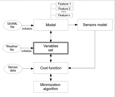
ReTrofiT is implemented as a Matlab toolbox [7]. Its object-oriented architecture provides theR
necessary modularity so that new model of algorithm components be easily added. Any CAD tool compatible with the standard gbXML data exchange format can be used to generate the building’s geometrical description using the specific import tool.
This paper presents the main characteristics of ReTrofiT software. The first section describes the building energy model. The next session describes the tools provided to set up and solve optimization problems. Finally, the last session illustrates the use of the software in typical applications related to heating load computations, sensitivity analysis and identification of non linear model parameters. 1. MULTIZONE MODEL AND DYNAMIC THERMAL SIMULATION
1.1 Modelling assumptions
The mathematical model describing the thermal state of the building builds upon standard multizone assumptions (see for instance [8] for details). The zone state variables are supposed homogeneous in the entire air volume. In each zone, the mean air temperature is governed by an ordinary differential equation with source terms related to internal gains, solar gains, and air mass exchange gains.
Air flows are considered in a simplified way, only air mass exchange between zones and with outside air due to infiltration effects are described.
Cj dTj dt −
∑
i C 0 i j−∑
i CL i j = Rjk(Tk− Tj) + Rej(Te− Tj) +ΓdjΦd+ ΓfjΦf + Qj+Wj+ η0jP Tj(0) = 0 (1)Table 1 : Description of terms
Expression Definition
Rjk(Tk− Tj) Air mass exchange between zone j and zone k; Rjk is an exchange coefficient, the
flow direction being set by the sign of the temperature difference (Tk− Tj)
Rej(Te− Tj) Air mass exchange between zone j and the outside
Γdj Solar gain coefficient (beam component) for zone j Γfj Solar gain coefficient (diffuse component) for zone j
Short wave solar radiation gains are taken into account through Γd j and Γ
f
j. They are computed
from the number of windows in the zone, the relative orientation and the window transmission coeffi-cient.
EWSHM 2014 - Nantes, France
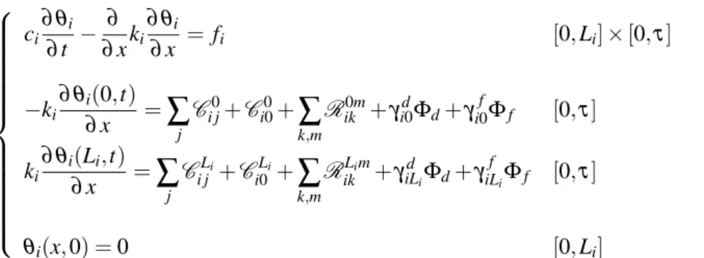
ci ∂ θi ∂ t − ∂ ∂ xki ∂ θi ∂ x = fi [0, Li] × [0, τ] −ki ∂ θi(0,t) ∂ x =
∑
j C 0 i j+Ci00+∑
k,m R0m ik + γ d i0Φd+ γ f i0Φf [0, τ] ki ∂ θi(Li,t) ∂ x =∑
j C Li i j +C Li i0 +∑
k,m RLim ik + γ d iLiΦd+ γ f iLiΦf [0, τ] θi(x, 0) = 0 [0, Li] (2)In the above expressions, xnand xmtakes the values 0 or Li depending of the surfaceorientation.
The table below gives the definitions of the various terms.
Table 2 : Description of terms
Expression Definition
Cn
i j= h0i j(θi(xn) − Tj) Convection terms between wall i (at x = xn) and zone j at
temperture Tj
Cn
i0= hni0(θi(xn) − Te) Convection terms between wall i (at x = xn) and outside air
at temperature Te
Rnm ik = α
nm
ik (θi(xn) − θk(xm)) Radiative transfer between wall i (at x = xn) and wall k (at
x= xm)
Rn∞
i j = βi j0(θi(xn) − T∞) Radiative transfer between wall i (at x = xn) and the outside
environment at temperature T∞
γind, γinf Solar coefficient of face x = xn of wall i, for the beam et
diffuse radiation
Heating device dynamics are governed by ordinary differential equation describing the evolution of the amount of heat Wjsupplied into zone j when some energy power Pjis injected.
dj dWj dt +Wj= ηjPj Wj(0) = Wj0 (3)
This generic model can represent, in a simplified way, both systems composed of standalone devices (eletric convectors for instance) and centralized heat production facilities.
Equations (1) to (3) constitute the standard system of equations in a typical energy simulation. As mentioned above, all equation terms are implemented as independent features that can be activated or disabled. These base equations can lead to different levels of details in the building model. Further, the software architecture enables future extensions of the system of equations with addition of new terms and equations, probably from other engineering fields.
1.2 Software architecture
ReTrofiT software is built in a modular way with object oriented programming. The building model constituting the core of the software is defined by a class containing all functions for mesh generation, matrix assembly and numerical integration. Each equation of the model is described into a separate object, which contains the implementation of all routines needed for the computation of its own terms. Those objects, called features, can be disabled on will, making it easy to adapt the level of detail.
In addition, this particular architecture makes it easy to add new terms in existing equations or new equations in the whole system of equations. The software can thus address problems related
to other engineering fields and could be viewed as a generic optimization platform for multiphysics applications, as the next section describes.
2. SOLVING OPTIMIZATION PROBLEMS 2.1 General formulation
It is a standard approach to formulate model calibration as a parameter identification problem [9]. Usually, a preliminary sensitivity analysis determines the model variables that have the highest impact on the computation of the quantities of interest. The parameter identification problem is an inverse problem that aims to determine the values of these predominant variables so that the gap between model simulation results and measured data be minimized. Such a problem is often ill-posed and needs an appropriate regularization procedure to be solved.
Problems of similar nature are also encountered in continuous monitoring applications: in this case, the unknown variables can be the initial state and/or the solicitations received by the system. The state estimation problem consists in identifying these unknowns using sensor data in order to reconstruct the global state of the system.
Optimal control for energy management applications provides another example of an optimiza-tion problem. In its simplest way, an optimal control problem consists in computing control laws (for example, power set-point of a heating device) to drive one or several state variables to a given set-point [10], [11].
All these problems can be formulated as minimization problems : one looks for a vector u such that
min
u∈Uc
J(u) (4)
where u is the control vector,Uc the control space that takes in account any additional constraints on
u. J is the cost functional which in a generic form writes J(u) = α1 2 kTu − yk 2 M+α22ku − u0k2U + α3 2 kφ (u)k 2 (5)
The first term of this expression is the so-called residue term. It measures the quadratic gap between the model response Tu and sensor data (or set-points, depending on the problem type) in the measurement spaceM . The model response Tu is obtained by applying an observation operator that models the measurement process on the solution of the partial derivatives equation system (1) - (3).
The second term is a weighting term for the control vector in a specific norm. In an identification problem, it acts like a regularization term avoiding the solution to be too far from an a priori guess . In this case, the weighting coefficient α2is called the Tikhonov parameter and must be small [6]. In an
optimal control problem, this term represents a measure of the energy cost. In this case, coefficients α1and α2reflects the trade-off between, for instance, the comfort represented by the first term and the
consumption represented by the second one.
The third term is a so-called penalization term enable to force the constraints. The function φ (u) is constructed such that it is (almost) null when u satisfies the constraints and positive otherwise. 2.2 Adjoint model
The minimum of the cost function J corresponds to the Euler conditions, i.e. to the point where the gradient is null. This minimum can be obtained using descent iterative methods.
The computation of the gradient of the second term is straightforward. The gradient correspond-ing to the computation of the third term depends on the function φ . In most cases, it is possible to choose a function for which the gradient is known explicitly.
EWSHM 2014 - Nantes, France
Computing the gradient calculation of the first term is less straightforward because the unknowns udoes not appear explicitly in the expression. Numerical differentiation should be avoided, because discretization of time dependent components of vector of unknowns u usually leads to a discrete vector of unknowns with a great number of components. Numerical differentiation would require at least one model resolution per discrete vector component which would dramatically increase computation cost. ReTrofiT natively implements the so-called adjoint model, which gives the exact gradient with only one adjoint resolution according to optimal control theory [12]. The adjoint model has the same structure as the direct model, meaning that the same numerical tools can be used for its resolution. 2.3 Minimization algorithms
Iterative descent algorithms of descents can be used to solve (4), each iteration requiring a resolution of the adjoint models to obtain the new gradient computation. ReTrofiT implements various descent algorithms exemplified in what follows.
When the model is linear with respect to all unknowns one can use the steepest descent or conju-gate gradient algorithm. The latter, applied to a functional of the form J(u) = 12kTu − yk2
M writes as
follows :
• Initialization : u0
• g0= T∗(Tu0− y), h0= −g0
• At each iteration n ≥ 1
– Compute optimal step : ρ = hn(g,Tn∗,hT hn)n)
– Compute descent direction hn: un+1= un+ ρhn
– Iteratively compute the gradient : gn+1= gn+ ρT∗T hn – Compute conjugate direction coefficient : γ = (gn+1(gn,g,gn+1n) )
– Iteratively compute the descent direction : hn+1= −gn+1+ γhn – Stop if (gn+1, gn+1) < ε
In case the model is non-linear with respect to some unknowns, a linearization step is required. The Levenberg-Marquardt algorithm is suited to this case. It consists in constructing, at each iteration, the following functional:
Jk(δ u) =
1
2kTuk+ δ T (δ u) − yk
2
M+ε2nkδ ukU (6)
and to minimize with respect to δ u. In the expression (6), δ T (δ u) is the response of the linearized model around the point uk such that: T (uk+ δ u) ∼ T (uk) + δ T (δ u). The minimum of Jk can for
instance be obtained with the conjugate gradient described above.
These algorithms can be adapted in the cases where bound constraints must be prescribed on the unknowns. In this case, an additional projection step is added at each iteration. For more general constraints more appropriate algorithms such as the Uzawa method or other dual algorithms should be used.
ReTrofiT software includes specific classes for all the above mentioned algorithms. Here again, the architecture is open to future addition of new algorithms.
3. APPLICATION EXAMPLES
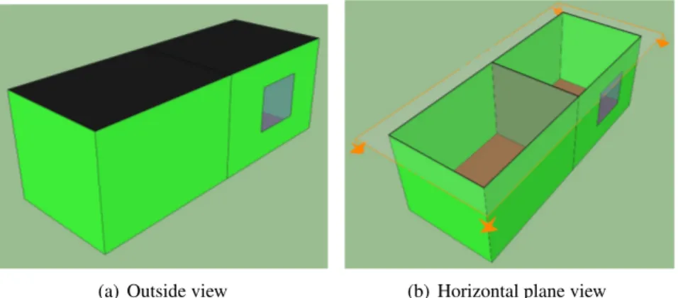
This section presents application examples on a test case in order to illustrate the various possibilities of the software. The case study is a building consisting of two zones, one of which includes an opening.
(a) Outside view (b) Horizontal plane view
Figure 1 : The case study building geometry: 3D geometry description using GSketchup CAD software
3.1 Computing heating loads and sensitivities
The theoretical heating loads during a time period [0, τ] can be computed by determining W that minimizes the cost function J(W ) given by
J(W ) =1 2
∑
j Z τ 0 (Tj− Tc)2dt+ ε 2∑
j Z τ 0 Wj2dtwhere Tjare the solutions of (1).
The sensitivity SW of W∗with respect to a parameter (for example, a perturbation δ Rej of the ir
exchange rates Rej) is given by
Find SW solution of minSWJ(SW), where
J (SW) = 1 2
∑
j Z τ 0 ( ˜Tj)2dt+ ε 2∑
j Z τ 0 (Wj∗)2dt Cj dTj dt −∑
i C 0 i j−∑
i CL i j = Rjk(Tk− Tj) + δ Rej(Te− Tj) T(0) = 0 (7)where the last equation is coupled to the linearized forms of equations (2) and (3).
The figure (2) gives an example of solutions of these two problems, obtained with ReTrofiT. 3.2 Resolution of an identification problem
The same tools can be used to formulation and solve an identification problem. Figure (3) gives an example where ambient air temperature measurements are used to reconstruct time-dependent air mass exchange. This result was obtained using the Levenberg-Marquardt algorithm with bound constraints were prescribed on the variable. The total computational time is around 11 seconds on a standard PC. CONCLUSION
ReTrofiT is a software for building energy simulation specially designed to solve optimization and identification problems applied to building energy management. It natively implements the adjoint model and includes various algorithm classes thus providing the user with a wide set of operational tools to formulate and solve optimization problems covering a wide range of engineering applications.
EWSHM 2014 - Nantes, France
Figure 2 : Computation of heating load and its sensivity with respect to a perturbation on air filtration rates.
(a) Ambient air temperature measurements (b) Reconstructed of air mass exchange
Figure 3 : Example of reconstruction of air mass exchange based on ambient air temperature measurements
The software architecture was designed to adapt to various situations by enabling the user to adapt the model’s level of detail and model’s complexity at will. It also enables future extensions of the software possibilities by addition of new resolution algorithms or model features, possibly related to other fields of physics.
REFERENCES
[1] T.A. Reddy. Literature review on calibration of building energy simulation programs: Uses, problems, procedures, uncertainty and tools. ASHRAE Transactions, 112(1), 2006.
[2] A. Nassiopoulos, R. Kuate, and F. Bourquin. Calibration of building thermal models using an optimal control approach. Energy and Buildings, 2014. Under press.
[3] Y. Heo, R. Choudhary, and G.A. Augenbroe. Calibration of building energy models for retrofit analysis under uncertainty. Energy and Buildings, 47(0):550 – 560, 2012.
[4] P. Bacher and H. Madsen. Identifying suitable models for the heat dynamics of buildings. Energy and Buildings, 43:1511–1522, 2011.
[5] M. N. Özisik and H. R. B. Orlande. Inverse Heat Transfer. Taylor and Francis, 2000.
[6] H. W. Engl, M. Hanke, and A. Neubauer. Regularization of Inverse Problems. Kluwer Academic Publishers, 1994.
[7] Mathworks. Matlab software,www.mathworks.com, 2012.
[8] J. A. Clarke. Energy simulation in building design. Butterworth Heinemann, 2001.
[9] J. Brouns, A. Nassiopoulos, F. Bourquin, and K. Limam. Identification de paramètres et séparation de sources thermiques à dynamiques différentes dans le bâtiment en utilisant la variation totale. In Congrès de la Société Française de Thermique, Gerardmer, France, July 2013.
[10] I. Hazyuk, C. Ghiaus, and D. Penhouet. Optimal temperature control of intermittently heated buildings using model predictive control: Part ii - control algorithm. Building and Environment, 51:388–394, 2012.
[11] F. Oldewurtel, B. Parisio, C. N. Jones, D. Gyalistras, M. Gwerder, V. Stauch, B. Lehmann, and M. Morari. Use of model predictive control and weather forecasts for energy efficient building climate control. Energy and Buildings, 45:15–27, 2012.
[12] J.-L. Lions. Contrôle optimal des systèmes gouvernés par des équations aux dérivées partielles. Dunod, 1968. Translation by S. K. Mitter: Optimal control of systems governed by partial differential equations, Springer, 1971.
EWSHM 2014 - Nantes, France