Configurations and Modulation Schemes Trade-off

CONFIGURATIONS AND MODULATION SCHEMES TRADE-OFF

(1)_{IAGL, Université de Liège}

17 Allée du 6 Août, B5C B-4000 Sart-Tilman, Belgium

Email: absil@astro.ulg.ac.be

ABSTRACT

During the preliminary phase A of the Ground-based European Nulling Interferometer Experiment (GENIE), a number of interferometric configurations have been studied, in the cases of exozodiacal cloud and hot Jupiter detection. Their expected performances have been computed in light of the measured or expected performances of the VLTI sub-systems. A simple Bracewell nulling interferometer, formed of two Unit Telescopes and working in the L’ or N bands, has been identified as a good candidate configuration for exozodiacal cloud detection. External or internal chopping, fringe tracking and intensity matching will be critical issues for this configuration. In the case of hot Jupiter detection, a double Bracewell with internal modulation in the L’ band seems well appropriate, and should allow to carry out low resolution spectroscopy on a few bright exoplanets. The basic assumptions and computations which have lead to these candidate configurations are described in this paper.

INTRODUCTION

The principle of nulling interferometry was proposed by R. Bracewell [1] in 1978. The purpose of this technique is to achieve a destructive interference for an on-axis target while letting through the signal from a nearby companion or a surrounding dust cloud. This can be achieved by introducing an achromatic π phase shift in one arm of the interferometer (Fig. 1). Nulling interferometry has been identified as one of the most efficient ways to directly detect the light coming from an extra-solar planet, and has been selected as a baseline for ESA’s Darwin mission.

Fig. 1. Principle of a Bracewell nulling interferometer.

Because a nulling interferometer uses coaxial beam-combination, no image is formed: the total flux coming through the interference pattern (also called transmission map) is integrated on a single pixel detector. It comprises the contributions from the scientific target (dust cloud and/or planet), from the residue of the stellar signal (called stellar leaks hereafter) and from the thermal background emission. Therefore, the contribution from the scientific target cannot be extracted from the total signal without an appropriate modulation scheme. Moreover, the stellar leaks and the thermal background are two important sources of shot noise and “fluctuation noise”, as explained below.

In the case of the Darwin mission, where Earth-like planet detection is the main goal, the light coming from the exozodiacal dust cloud (exozodi) surrounding the target star is also a source of noise, and could become the dominant one if the dust density around the target star was about 10 times higher than around our own Sun (“10-zodi” level). The characterization of the amount of dust around the candidate targets of Darwin is therefore an important task for a

precursor mission as GENIE. The instrument should be sensitive to exozodiacal dust clouds 10 times denser than our local zodiacal cloud. The reference target for GENIE will therefore be a 10-zodi cloud surrounding a Sun-like star at 10 parsecs. Table 1 summarizes the integrated fluxes from the star and the dust cloud in the four infrared atmospheric windows considered in this preliminary study. The exozodiacal cloud model developed by Kelsall et al. [6] has been used. The typical field-of-view of a fibre-linked interferometer is given by the relation Ω = λ2 _{/S (with S the telescope}

surface), and corresponds to a few AU for mid-infrared observations of a target at 10 pc. Therefore, only the hot inner part of the cloud is detected. Note that this field-of-view is large enough to include more than 90% of the infrared flux from the exozodiacal could, because most of the flux comes from the hot inner zone.

Table 1. Infrared flux from the reference target (10-zodi cloud around a Sun-like star at 10 parsecs) in the interferometric field-of-view of a 8-m telescope.

Waveband K L’ M N Wavelengths (µm) 2.0 – 2.4 3.5 – 4.1 4.5 – 5.1 7.7 – 12.7 Sun at 10 pc (Jy) 28 12 8.5 2.2 Corresponding magnitude 3 3 3 3 Exozodi (mJy) 0.2 0.5 0.6 1.0 Corresponding magnitude 16 14 13 11 Star/exozodi ratio 1.4 × 105 _{2.4 × 10}4 _{1.6 × 10}4 _{2.2 × 10}3

NULLING CONFIGURATIONS AT THE VLTI

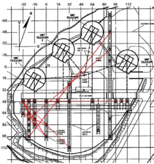
Thanks to its four 8-m Unit Telescopes (UT) and its three 1.8-m Auxiliary Telescopes (AT) which move on tracks (a fourth AT will probably be built), the VLTI offers a great number of potential nulling configurations. Some of them are appropriate for exozodiacal cloud detection, while others are specifically designed to detect extra-solar planets. In any case, linear arrays are generally preferred, because their projection on the plane of the sky remains homothetic during the night, while 2-D configurations are deformed by Earth rotation. A map of the VLTI site is presented in Fig. 2, where the AT stations are represented by black dots. Note that two ATs cannot be used simultaneously on the same “vertical” track, because in that case the light beams cannot be sent simultaneously to the delay lines.

Fig. 2. Map of the VLTI site. The red lines show all the possibilities to find three aligned AT stations. Configurations for exozodiacal cloud detection

In order to detect exozodiacal dust around nearby stars, simple nulling configurations like a two-telescope Bracewell interferometer formed of two UTs can be used. In that case the transmission map of the interferometer (Fig. 3) lets through about 40% of the total exozodiacal emission. Other contributors to the total signal are the stellar leaks, the

thermal background and a potential planet orbiting the target star. Unless this planet is a hot giant planet (a “51 Pegasi” planet), its thermal emission will be negligible compared to the infrared flux from the exozodiacal cloud.

Fig. 3. Left: Transmission map a Bracewell interferometer (50 m baseline) in the interferometric field-of-view of a 8-m telescope. The brightest zones denote a transmission of 100%.

Right: Horizontal cut through the central transmission, showing a θ2 _{central dependence.}

The right-hand side of Fig. 3 shows that the null of a Bracewell interferometer is not very deep: the central transmission is proportional to θ2 _{if θ is the angle to the axis. Therefore, a wide fringe pattern is recommended to cancel the starlight}

as much as possible.

Other linear configurations cannot be found with the Unit Telescopes. On the other hand, three or even four aligned AT stations can easily be found (see Fig. 2). It is therefore possible to use nulling configurations with a deeper null, like the DAC and OASES configurations (Fig. 4). Their central transmission scales respectively as θ4 _{and θ}6_{. These}

configurations will thus produce a lower stellar leakage, which could be a serious advantage if the calibration of the stellar signal turns out to be a limiting factor. The main drawbacks of these configurations is that the recombination scheme is more complex and that only the 1.8-m Auxiliary Telescopes can be used, leading to a lower sensitivity.

Fig. 4. Left: Aperture configuration of a DAC nulling interferometer, and its central transmission. Right: Aperture configuration of an OASES nulling interferometer, and its central transmission. The light and dark grey fillings represent respectively a 0 and a π phase shift applied to the beams. Configurations for hot Jupiter detection

In the case of exoplanet detection, the light coming from the exozodiacal cloud is an additional source of noise, and should be removed for a secure detection. A special modulation technique, called internal modulation, has been designed by Mennesson and Léger [7] for this purpose. This technique has the advantage to remove all spurious signals, such as the background, mean stellar leaks and exozodiacal light. Internal modulation could be tested at the VLTI in a “double Bracewell” configuration. Its principle is illustrated in Fig. 5.

Fig. 5. Principle of internal modulation: the double Bracewell interferometer.

The principle of internal modulation is to use two (or more) nulling interferometers in order to perform fast modulation between their outputs. By recombining the outputs of two Bracewell interferometers on a loss-less beam-combiner, we get two transmission maps which are both asymmetric, although symmetric to each other with respect to their centre. Therefore, all sources with central symmetry such as the exozodiacal cloud, the background and even the mean stellar leaks have the same contribution in both outputs. On the other hand, the planet has two different contributions because when it is located on a bright zone in the first map, it is on a dark zone in the second map. Thus if we alternately detect these two outputs, we get a final signal where only the planetary part is modulated. The modulation map shows which places on the sky are strongly modulated (bright zones), and where there is no modulation at all (dark zones).

MAIN NOISE SOURCES

The noise coming from the stellar leaks and the thermal background can both be divided into two parts: the shot noise associated to their mean value, and the noise associated to their fluctuations. In the case of stellar leaks, the fluctuations are due to two main effects: differential optical path delay between the two arms of the interferometer, and intensity mismatches in the two arms of the interferometer. In the case of thermal background, the fluctuations are mainly due to temperature and emissivity fluctuations in the atmosphere and in the optical train.

In this section, the main sources of “fluctuation noise” are presented, in the case of a Bracewell interferometer. We also investigate some ways the remove the mean stellar leaks and background. These considerations can easily be generalised for a nulling interferometer formed of more than two apertures.

Atmospheric piston

A major source of stellar leaks fluctuations is the time-varying optical path delay (OPD hereafter) between the two arms of the interferometer: the non-homogeneity of the atmospheric refraction index induces a differential delay between the two incoming wavefronts referred to as “piston” (Fig. 6). The piston is highly variable with time, with a zero mean and a typical standard deviation of 20 µm RMS for a 40 m baseline.

The effect of differential OPD is to make the fringes move around their central position (Fig. 7). In the case of GENIE, this means that the central dark fringe is not centred on the stellar disk any more, so that the starlight transmission increases. In the N band, an OPD variation of 5 µm is sufficient to get a constructive interference instead of a destructive one, and therefore, the differential OPD must be reduced by means of a fringe sensing unit (FSU). The nulling process needs a very high stability in the position of the fringes, particularly at short wavelengths. Fringe stabilisation will be achieved by the PRIMA-FSU facility at the VLTI.

Fig. 7. Left: The central fringe moves around the centre of the field-of-view as a result of OPD fluctuations. The size of the stellar disk is about 0.5 mas in radius for a 10 pc Sun-like star.

Right: Mean transmission, averaged on 100 random values of the differential OPD.

At the output of the FSU, the residual piston is characterised by its power spectral density (PSD). In this section, a simple FSU model (see [6]) is used in order to get an approximate PSD of the residual OPD. This PSD is the key to assess the fluctuations of the stellar leaks. The specifications of the FSU in [6] show that, for a guide star of magnitude K=7, the RMS residual OPD at the output of the fringe tracker will be about 11 nm RMS (this limit comes from the OPD measurement noise). But since the magnitude of a Sun at 10 pc is about K=3, the fringe sensing could be optimised for brighter targets in order to get a lower residual OPD. This is not expected for the PRIMA FSU, but could well be implemented inside the GENIE instrument, as a second level of fringe tracking. Preliminary simulations show that the limit performance of a FSU on bright stars should be about 7 nm RMS.

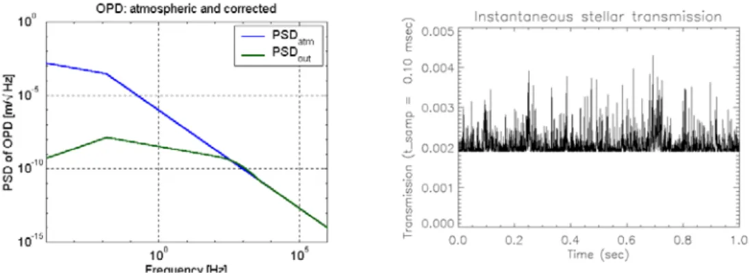
In this study, we have used a repetition frequency of 4 kHz for the fringe sensor and the FSU noise specified in [6]. Delay line noise has not been added. The residual OPD in closed loop was of 16 nm RMS in that case. The inferred stellar transmission is shown in Fig. 8, for a Bracewell interferometer working in the L’ band. The mean stellar transmission is of 0.002 and the RMS transmission of 5×10-5_.

Fig. 8. Left: Simulated power spectral density for the atmospheric and the residual piston.

Right: Instantaneous stellar transmission taking OPD fluctuations into account, computed in the L’ band for a Bracewell interferometer of 47 meters.

Intensity mismatch

If the intensities in the two arms of the interferometer are not equal, the on-axis transmission is not null any more, as proven by the interferometric equation:

1 2

2

cos(

)

I

= + +

I

I

I I

φ φ

−

where I1 and φ1 (resp. I2 and φ2) are the intensity and phase for the first (resp. second) light beam. If I1 ≠ I2, the intensity

does not cancel any more, even if φ2 – φ1 = π. There is a vertical deformation of the central fringe, as seen in Fig. 9. The

main cause of intensity mismatch is the atmospheric turbulence across a single telescopes pupil. If σφ1 and σφ2 are the

RMS phase variations over the two independent pupils, the intensities coupled from telescopes 1 and 2 into single-mode fibres can be written:

2

1 0

exp(

)

I

=

I

−

σ

I

=

I

exp(

−

σ

)

where the exponential factor represents the coupling efficiency into the fibre, which only accepts the coherent part of the incoming beam. The MACAO adaptive optics system [4] will equip all of the four Unit Telescopes by end of 2004. The quality of the wavefront correction by the AO system is measured by the Strehl ratio, which will be of about 0.64 in the case of a bright star (mV=9) observed in the K band (B. Koehler, personal communication). The corresponding

coupling efficiency, including the tip-tilt effect, will be about 0.58, with an RMS of 0.12. The effect of unmatched coupling efficiencies in the two arms of the interferometer is presented in Fig. 9, where we have chosen typical values of 0.52 and 0.64 for the coupling efficiency. Note that the coupling efficiency depends exponentially on the wavelength: since the RMS phase variation across the pupil is proportional to 1/λ, the coupling efficiency will be larger at longer wavelengths, and its fluctuations lower.

Fig. 9. Deformation of the fringe pattern due to unmatched coupling efficiencies in the two arms of a Bracewell interferometer. The left-hand figure shows that the total transmission is reduced due to the mean coupling

efficiency of 0.58, while the right-hand figure shows the vertical deformation of the central fringe.

The time variations of the coupling efficiency induce a variation of the stellar leaks, which is an important source of noise, particularly at short wavelengths. It would be the dominant source of noise unless an intensity matching device (IMD) is used to reduce the intensity mismatch. As in the case of the FSU, the IMD is characterised by its transfer function, and by the output power spectral density of the coupling efficiency fluctuations.

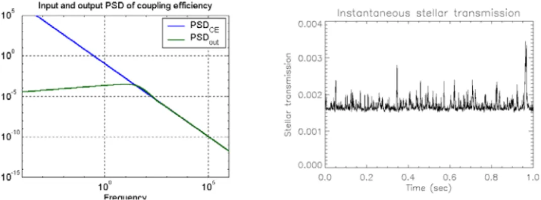
Simulations of the MACAO adaptive optics system have shown that the power spectral density of the uncorrected coupling efficiency fluctuations has a slope of –1.8 (B. Koehler, personal communication). A feedback loop with a simple integrator can be used to reduce the low-frequency component of the coupling efficiency fluctuations. When operating in the K, L’ or M bands, a repetition frequency of 300 Hz is sufficient to reduce the intensity-induced stellar leaks fluctuations down to the piston-induced fluctuations. When operating in the N band, where the fluctuations are much lower, a repetition frequency of 1 Hz is sufficient. This is illustrated by Fig. 10, obtained in the L’ band. The initial RMS coupling efficiency was of 0.07. After correction by the IMD (at 300 Hz), the RMS coupling efficiency goes down to 0.02. The associated RMS stellar leakage is of 1.2×10-4_{, which is of the same order than the OPD-induced}

Fig. 10. Left: Simulated power spectral density for the uncorrected and residual coupling efficiency fluctuations. Right: Instantaneous stellar transmission taking coupling efficiency fluctuations into account, computed in the

L’ band for a Bracewell interferometer of 47 meters. Calibration of stellar leaks

The fundamental limitation of a nulling interferometer is that its transmission is equal to zero only on the axis, while the star has a finite angular extent. Therefore, a small fraction of the light coming from the limb of the star will leak through the null, and produce a spurious signal at the detector. The amount of stellar light incoming on the detector depends on the quality of the nulling process, i.e. on the chosen configuration and wavelength. The last line of Table 1 shows that, in order to reduce the stellar signal down to the exozodi signal, the stellar transmission should be about 10-5 _{in the K}

band, 10-4 _{in the L’ and M bands, and 10}-3 _{in the N band. The N band is therefore preferred regarding stellar leaks, all}

the more because the fringe pattern scales as the wavelength, so that the central dark fringe is wider in the N band than in the near infrared.

Four possible ways to separate the exozodiacal signal from the stellar leaks have been considered:

1. A priori calibration: If the stellar diameter is known with a good precision from theoretical models or previous

observations, one can compute the theoretical stellar leaks and subtract this amount from the total signal in order to retrieve the signal of the exozodiacal cloud. This method has a low precision since the actual stellar transmission is generally higher than the theoretical one, because of atmospheric turbulence (as explained above). The expected calibration precision is of about 10%.

2. A posteriori calibration: This calibration method is an improvement of the previous one: instead of using the

theoretical transmission map, we will use the error estimates from the FSU (residual phase error) and from the IMD (residual intensity mismatch) in order to compute the actual stellar transmission. This could lead to a much better calibration precision, which is still to be computed.

3. Spectrum subtraction: This technique assumes that some spectral resolution will be available in GENIE. The idea

is to get a spectrum of the star through GENIE in a non-nulling mode, and to subtract the stellar spectrum from the scientific data. The accuracy of such a method is highly dependent on the spectral resolution achievable (and thus on the level of the exozodiacal flux) and on the stellar type. It has not been evaluated yet.

4. OPD modulation: Another way to remove the stellar contribution in the output signal is to modulate this

contribution at a known frequency. This could be achieved by slightly moving the dark fringe around the centre of the field-of-view by OPD variations. The amplitude of the OPD modulation must be larger than the residual OPD from the FSU in order to get a “deterministic” modulation of the stellar leaks. The main drawback of this method is that the mean stellar leakage increases drastically, and so its associated shot noise.

In any of the four cases, further investigations are needed to assess the precision of stellar leaks calibration. The prospective performances of the instrument presented in the next section do not take the stellar calibration into account: we have assumed a perfect removal of the stellar leaks. The final ratio of exozodiacal flux to stellar leaks will however give us an important information on the precision of stellar calibration to be reached.

Thermal background

An important source of noise for any ground-based infrared observation is the thermal emission from the sky and from the telescope itself. The atmospheric background has been measured in several astronomical sites. The values in Table 2 are based on measurements carried out on Mauna Kea. They are consistent with an atmosphere at 245 K, and with

recent observations of Cuby et al. [2] at Cerro Paranal. The thermal emission from the warm optical surfaces depends on their emissivity and temperature. We have computed a theoretical emissivity of 50% for the whole VLTI optical train, which is probably somewhat optimistic because the dust which might settle on the mirrors could increase their emissivity. The mean temperature in the VLTI interferometric lab and delay line tunnel is about 288 K. The GENIE instrument is not expected to contribute to the thermal emission because it will be cooled by a cryostat.

Table 2. Mean thermal background, compared to the exozodiacal flux (10-zodi cloud around a Sun at 10 pc). The estimated integration times are computed for a signal-to-noise ratio of 3 and only take into account the shot noise

from the background and the exozodi. A total transmission of 5% is assumed for the GENIE instrument.

Waveband K L’ M N

Exozodi (mJy) 0.2 0.5 0.6 1.0

Mean sky brightness (Jy/as2_{) 0.004 3 30 400} Blackbody at 288 K (Jy/as2_{) 0.012 32 251 6567}

Interferometric FOV (as2_{) 0.004 0.012 0.019 0.088} Background / exozodi 0.7 2×103 _2×104 _1×106 U

T

Estimated integration time (sec) 7×10-4 _{0.3 2 285} Interferometric FOV (as2_{) 0.081 0.24 0.38 1.7}

Background / exozodi 13 3×104 _4×105 _2×107 A

T

Estimated integration time (sec) 0.1 100 700 1×105

In addition to its shot noise, the background contributes to the total noise by its time fluctuations. Chopping is a technique designed to get rid of the background emission and of its fluctuations by alternately measuring the flux from the scientific source and from a nearby sky region, in order to sample the background emission. In fact, little is known about the stability of the background, particularly in the mid-infrared. In the following calculations, we will always assume that the chopping is efficient enough to remove the background fluctuations. This may not be the case in practice, unless a high chopping frequency is used (at least 5 Hz).

Two chopping techniques have been considered in the case of GENIE. The first one is the classical chopping method (or external chopping), where the secondary mirror of the telescope is tilted at a frequency of 0.1 to a few Hz. The main drawback of this simple chopping scheme is that at each time the secondary is tilted to sample the background, the tip-tilt unit (STRAP), the adaptive optics system (MACAO) and the fringe sensing unit (PRIMA-FSU) do not see the guide star any more, and therefore cannot remain in closed loop. Consequently all these sub-systems have to re-close their loops before each single interferometric measurement can be made. The overall efficiency of the chopping process will thus critically depend on the efficiency of these sub-systems, which are expected to close their loops in a few hundreds of milliseconds, while a chopping period last typically for 100 ms. The percentage of time spent on the scientific target will therefore be quite low. A potential improvement of this technique is to use counter-chopping, so that STRAP and MACAO can keep their loop closed during the chopping. The FSU would still have to re-acquire the fringes at each interferometric measurement.

The second chopping method is called “internal chopping”, and uses a phase modulation as proposed by Kuchner and Serabyn [5]. In this chopping scheme, the pupil of the two telescopes are divided into two parts. The principle is then to recombine the first (resp. second) half of telescope 1 with the first (resp. second) half of telescope 2 with a nulling interferometer, and to combine the two nulled outputs with a time-varying phase shift (see Fig. 11). The result is a set of baselines of two different types: long (46 m) baselines between the corresponding sub-apertures of the two UTs, and short (3.4 m) baselines between the two halves of each UT. The two beam-combinations produce two perpendicular fringe patterns, with respective periods of λ/46 and λ/3.4 (resp. equal to 45 mas and 618 mas at λ = 10µm). Fig. 11 illustrates how internal chopping can be used to remove the background emission from the scientific data: if φ = π/2, the final beam-combiner produces a constructive on-axis interference for the first output, and a destructive on-axis interference for the other output. The contribution of the exozodiacal cloud will therefore be different in the two outputs, while the incoherent background has the same contribution in both of them. Subtraction of the two output signals can thus be used to cancel the background emission. Note that the chopping frequency is not limited by the movement of a flipping mirror any more. Moreover, all sub-systems can keep their loops closed during the “virtual” chopping. The main drawback of this chopping method is that it increases the complexity of the instrument.

Fig. 11. Principle of internal chopping, based on the original concept of Kuchner and Serabyn [5]. EXPECTED PERFORMANCES

Prospective performances of the GENIE instrument have been computed, taking into account the noise sources discussed above, as well as the read-out noise of current infrared detectors. The noise contributions are presented in Fig. 12 in the case of L’ and N band observations. As expected, the background is the dominant source of noise in the N band, where the detector noise has also an important contribution. In the L’ band, the “fluctuation noise” due to stellar leaks becomes an important contributor. It would become dominant if the performances of the fringe sensing unit or of the intensity matching device were worse than expected. Current performance estimates for the PRIMA-FSU give a residual OPD error of 50 nm RMS. This is much larger than the residual of 16 nm RMS assumed in our simulations. Therefore a second (more accurate) stage of OPD control would probably be needed for L’ band operation.

Fig. 12. Noise contributions for a UT2-UT3 Bracewell interferometer pointing at zenith towards a Sun-like star at 10 pc surrounded by a 10-zodi cloud. Legend: ⋅ ⋅ ⋅ ⋅ ⋅ photon noise from the exozodi and from the mean stellar

leaks, –––– background noise (assumption: only photon noise), – – – fluctuation noise due to leakage fluctuations, – ⋅ ⋅ – detector read-out noise (40 electrons RMS in L’, 1000 electrons RMS in N).

The expected performances of the Bracewell interferometer are summarised in Table 3. They prove that the detection of 10-zodi clouds around nearby stars is a realistic goal, within less than one hour of integration time. Depending on the chosen waveband, we will face different kinds of problems: background emission at long wavelengths (M and N bands) and stellar leaks at short wavelengths (K and L’ bands). The first problem cannot be solved, unless bigger telescopes are available, while the second problem can be tackled by using other types of configurations. The DAC and OASES configurations, which have a deeper null, would reduce the contribution of the stellar leaks by a factor of about 10. Better rejection rates are not achievable due to piston and intensity mismatch. However, the DAC and OASES configurations require Auxiliary Telescopes to be used. As proven in Table 2, this increases the background to exozodi ratio by a factor of 20. The resulting integration times would be too long in the M and N bands. On the other hand, K or L’ band operation is possible thanks to the lower thermal background.

Table 3. Prospective performances of a Bracewell interferometer formed of UT2 and UT3: signals (ph-el) and noises (ph-el rms) in 100 seconds for a 10-zodi cloud around a Sun at 10 pc.

K band L' band M band N band

EZ signal 6.6e4 1.9e5 1.8e5 1.4e6

Star transm. 4.1e-3 1.8e-3 1.2e-3 2.9e-4

Star signal 1.5e8 2.5e7 7.7e6 2.0e6

Back. signal 4.6e4 2.7e8 2.6e9 1.1e12

Phot. noise 1.2e4 5.0e3 2.8e3 1.8e3

Back. noise 2.1e2 1.6e4 5.1e4 1.1e6

Trans. noise 1.2e5 2.0e4 5.8e3 3.5e3

Det. noise 1.3e3 1.3e3 3.8e3 3.4e5

SNR 0.53 7.6 3.6 1.2

In the case of hot Jupiter detection, the signal-to-noise ratio depends on the chosen target. For the brightest exoplanets (tau Boo b, 51 Peg b), we can expect the signal-to-noise ratios to be somewhat larger than those in Table 3, especially in the near-infrared where a 100 m baseline is sufficient to resolve the star-planet system. The N band is not really appropriate for hot Jupiter detection at the VLTI, because the typical angular distance between the star and the planet is of 5 mas, while the angular resolution is limited to 20 mas in the N band.

CONCLUSIONS

The choice of the waveband for GENIE is a crucial issue. We have to chose between large stellar leaks in the near-infrared and a huge thermal background in the mid-near-infrared. The N band has two important advantages: first, it corresponds to the Darwin waveband, so that any technological development would be beneficial to the space mission, and second, it is probably more suited for scientific exploitation thanks to the interesting spectral features in the 8-12 µm region (silicates, …). On the other hand, the L’ band allows the use of Auxiliary Telescopes for scientific observations, and would probably be more representative of the Darwin environment, where the background and the stellar leaks have almost the same level. The L’ band could also allow the use of an integrated optics beam-combiner. The choice of the aperture configuration is probably more straightforward: the Bracewell configuration is recommended because of its simplicity. Due to the increased complexity of their recombination scheme, the DAC and OASES interferometers would only be recommended if the stellar leaks calibration turns out to be a major issue. Once again, in order to reduce the complexity, external chopping is recommended, provided that it can achieve the required accuracy of background subtraction.

Finally, testing internal modulation with the double Bracewell configuration would be a major step towards Darwin, especially for data reduction in a Darwin-like environment.

REFERENCES

[1] Bracewell R., “Detecting nonsolar planets by spinning an infrared interferometer”, Nature, vol. 274, p. 780, 1978. [2] Cuby J., Lidman C. and Moutou C., “ISAAC: 18 months of Paranal Science Operation”, The Messenger, vol. 101,

p. 3, 2000.

[3] Kelsall T. et al., “The COBE diffuse infrared background experiment search for the cosmic infrared background. II. Model of the interplanetary dust cloud”, ApJ, vol. 508, pp. 44-73, 1998.

[4] Koehler B. and Gitton P., “Interface Control Document between VLTI and its Instruments”, VLT-ICD-ESO-15000-1826, Issue draft 3.0, December 2001.

[5] Kuchner M. and Serabyn E., “Modelling exozodiacal dust detection with the Keck interferometer”, ApJ, in press. [6] Ménardi S. and Gennai A., “Technical Specifications for the PRIMA Fringe Sensor Unit”,

VLT-SPE-ESO-15740-2210, December 2001.

[7] Mennesson B. and Léger A., “Direct detection and characterization of extrasolar planets: the Mariotti space interferometer”, unpublished.