Gérer le risque d'échantillonnage en économétrie financière : modélisation et contrôle

Gérer le risque d’échantillonnage en économétrie financière:

modélisation et contrôle

par

Bertille Antoine

Départementde sciences économiques Faculté des arts et des sciences

Thèse présentée à la Faculté des études supérieures en vue dc l’obtention dci grade de Philosophiae Doctor (Ph.D.) en scienceséconomiques, option économétrie et économie financière

Anut 2t)t)7

de Montréal

Direction des bibliothèques

AVIS

L’auteur a autorisé l’Université de Montréal à reproduire et diffuser, en totalité

ou en partie, par quelque moyen que ce soit et sur quelque support que ce

soit, et exclusivement à des fins non lucratives d’enseignement et de

recherche, des copies de ce mémoire ou de cette thèse.

L’auteur et les coauteurs le cas échéant conservent la propriété du droit

d’auteur et des droits moraux qui protègent ce document. Ni la thèse ou le

mémoire, ni des extraits substantiels de ce document, ne doivent être

imprimés ou autrement reproduits sans l’autorisation de l’auteur.

Afin

de

se

conformer

à

la

Loi

canadienne

sur

la

protection

des

renseignements personnels, quelques formulaires secondaires, coordonnées

ou signatures intégrées au texte ont pu être enlevés de ce document. Bien

que cela ait pu affecter la pagination, il n’y a aucun contenu manquant.

NOTICE

The author of this thesis or dissertation has granted a nonexclusive license

allowing Université de Montréal ta reproduce and publish the document, in

part or in whole, and in any format, solely for noncommercial educational and

research purposes.

The author and co-authors if applicable retain copyright ownership and moral

rights in this document. Neither the whole thesis or dissertation, nor

substantial extracts from it, may be printed or otherwise reproduced without

the author’s permission.

In compliance with the Canadian Privacy Act some supporting forms, contact

information or signatures may have been removed from the document. While

this may affect the document page count, it does flot represent any loss of

content from the document.

Université de Montréal Faculté des études supérieures

Cette thèse intittilée

Gérer le risque «échantillonnage en économétrie financière:

modélisation et contrôle

présentée par

Bertille Antoine

a été évaluée par un jury composé des personnes sui\ antes

Président-rapporteur

Caa

o

Directeur de recherche Eric

Examiniteurexterne

Alastai.r Hall—Univ. of Manchester

Ofôïa Rd

Membre du jury

Mc

Sommaire

L’objet dc cette thèse est le traitement de contextes d’application, en particulier dans le do

maine de l’économie financière, où lepointde vue asymptotique traditionnel peut être trom—

peur. Chaque essai propose alors crue méthode potir alhner les approximations asymptotiques en présence d’échantillons d’ohsers ations qtu, en pratique. sont tocmjocmrs finis.

Le premier essai se place dans la lignée de la littérature récente sur les instruments faibles.

Nous adaptons le contexte général de la méthode des moments généralisée (GMM) afin de lier plus spécifiquement la faible identification acix instruments, c’est—à—dire atix conditions

de moment. Ainsi, contrastant avec la plupart des méthodes existantes, la partition d’intérêt

entre les paramètres structurels fortement et faiblement identifiés n’est pas spécifiée a priori elle s’obtient plutôt après une rotation dans l’espace des paramètres. Par ailleurs, nous nous concentrons ici scir le cas d’identification presqcme-faihle potir lequel la déficience de rang est atteinte à la limite à un taux de conergence plus lent que l’usuel racine-i. Dans ce contexte,

les estimateurs GMM de tous les paramètres convergent, à des taux possiblement plus lents

que d’habitude. Cela nous permet de valider les approches de test standard comme Wald ou GMM-LM. De plcms, nous identifions et estimons des directions dans l’espace des paramètres pour lesquelles la convergence au taux racine—i est maintenue. Ces résultats sont d’un intérêt direct pour les applications pratiques. et ce, sans que la connaissance ou l’estimation du taux

de convergence plus lent ne soit mequmise. Nous proposons des illustrations Monie—Carlo pour dccix modèles économétriques le modèle dc régression linéaire avec variables instrLmmentales à une équation et le modèle d’évaluation d’actifs CAPM avec consommation.

Le deuxième essai complète le premier en réalisant une éttide comparative de puissance pour

deux tests de ta littématumre GMM avec instruments (presque)—faibles: le test de score clas sique, valide dans le cadre dti pi-emier essai, et le test de Kteihemgen oti score modifié. Plus

généralement,nous comparons_{deux approches: d’une part, à l’image du}premier essai, spé

cifier les problèmes d’identification, via le comportement des conditions de moment, permet

d’appliquer les procédures de teststandard: d’autre part, comme dans Kleihergen(2005), ne pas préciser e cadre d’identification requiert une moditication de la statistique du score. Dans le troisième essai, nous ptoposons une nouvelle méthode d’ inférence, la procédure Modihed-Wald, afin de pallier au mauvais comportement (connu) des tests de Wald lorsque l’identification n’est plus assurée à la fiontière de l’espace des paramètres. Nous nous concen— trons ici stir le ratio de paramètres multidimensionnel lorsque le dénorninateurest proche de la singularité. Notre méthode est basée stir la statistique de Wald : le contenu informationnel de l’hypothèse nulle d’intérêt est intégré dans le calcul de sa métricfue. Cette correction préserve la tractahilité dc la méthode et permet d’obtenir une région de confiance non bornée lorsque nécessaire. La procédure de Wald standard produit habituellement une région de confiance bornée: celle—ci est invalide pour toute taille d’échantillon donnée dans la mesure où sa pro babilité de cou\erture est nulle. La seule manière de remédier à ce problème est d’obtenir des régions de_{confiance non bornées avec une probabilité non nulle. Une simulation compare les} propriétés d’inférence des procédures Wald et Modified-Wald avec un ratio bidimensionnel. Nous considérons ausst le modèle de régression linéaire avec variables instrumentales à une équation lorsque les propriétés identifiantes des instruments varient.

Pour finit, contrastant avec lestrois premiers essais qui restent dansle domaine de la théorie statistique asymptotique. le quatrième essai adopte tin point de vue décisionnel dans le do maine dii choix dc portefeuille. Un défi important associé à l’allocation de portefeuille se pro— dtnt lorsque les caractéristiques (inconnues) de la distribution des rendements financiers sont remplacés par des estimés. Cela introduit du risqtic dit d’estimation, crucial pour la gestion (le portefeuille, au même titre qtie le risque financier traditionnel. Cet essai se concentre scir une nouvelle inescue de perfbrmance par rapport à la littérature existante. Nous empruntons aux praticiens et évaluons les différentes allocations de fonds à travers leur vraisemblance à battre un_{niveau de référence donné. Ensuite, le portefeuille optimal. qui incorpore alors le risque} d’estimation, est connu explicitement et ne dépend d’aucun paramètre de nuisance. Une étude de Monte—Carlo simple compare plusieurs stratégies d’investissement de la littérature. Mots clés: GMM: variables instrumentales: identification fpresque)—faihle : test K: test du score: ratio de paramètres: Wald : région de confiance non bornée: théorie du portefeuille: risqcie d’estimation : performance de référence : efficacité moyenne-variance.

Summary

The ehjectie cf this thesis is te stcidy designs. particularly in the Hcid e1 linancial ecenomics. wheretheasymptotic peint_{cf view may be misleading. Each essay proposes a rnethod te re} une the asy mptetic approximations in die presence of samples which are. in practice. aRvays dnite.

The lirst essay is in une with the recent literature en weak instruments. We propose te adapt ihe general framework cf ihe Gcneralized Method cf Moments (GMM) in eider te specifi cally relate weakness te the instrtlrnciits. that s the moment conditions. As a censequence.

n contrast with mest of theexisting literature. the relevant partition hetween stronglyand weakiy identified structurai pararneters is net specified a priori but rather achieved after a well-suited rotation in the parameter space. In addition. we focus here on the case duhhed ncarly-weaL identilication where the drifting DGP introduces a limit rank deticiency reachcd at a rate siower than reet-T. This framewerk ensures that the GMMestimatersof ail parame ters are consistent but at raies which may he slewer than usual. This altews us te veriIv the validitye! the standard tesiing approiiches like Waid and GMM-LM tests. Mereover. we iden

tify and estirnate directions in the parameter space where reot-T convergence is rnaintained. These resuits are ail directly relevant for practical applications without requiring knowledge or estimation cf the slower rate et cenveigence. We provide Monte—Carie illustrations fer two econometric medels: the single—equation I inear iV mode! and the consumpt ion hased CÀPM. The second essay cempletes the first ene with a comparative study of the power o! iwo tests proposed within the GMM literature when the ideniilication is (neariy)—weak: the standard score test. valid _{in the framewerk of chaptcr I. and the K-test or modilied score test. in n} more general sense. we are cemparing two approaches with respect te ideoiihcation issues: en _{one hand. as shown in the lirst essav. specifying identitication issues threugh moment}

iv

conditions allows the application o! standard test procedures: onthe other hand, as sho n hy Kleibergen (2005). in thc absence of identitication issLie specification a modification ol the score test statistic Sreqttired.

In ihe third essay. we propose u new int’ercnce method, the Moditied-Wald procedure. to over come some issues of the welt-documented pool hehavior of WaId tests when identilication is Iost at the frontier of the parameter space. We focus here on the mtiltidimensional ratio of parameters when the denominator is close to singularity. This method is hased on the Wald statistic. The key idea consistsofintegrating the informational content of the nul! hypothesis ot’ intetest n the computation of ils metric. This correction. while preserving thc computa— tional tractahility o! the rnethod. alloss for unhounded confidence regions when nceded. A standard Wuld test usually providesa bounded confidence region: this region is invalid forany

given sample sizeinthe sense that its couerage probahilitv iszero. The only svayto stirmolint this issue isto write conhdence regions with u non;em prohahility o! heing unhotinded. A simulation exercise compares the nlerenccpropcrlies of the Wald and Modified-Walcl pro cedures with a hidimensional ratio. We also consider the single-equation linearIV model in cases where the identifying properties of the instruments may vary.

Finalty. in contrasi to the first three essays which remain in the framework of statistical asymptolic theory. the fourth essay adopts a decisional point of view in portlolio choice. An important challenge in portfolio allocation arises ss lien the Ortie) characteristicso! re—

turns distrihution are replaced hy estimates. This introduces estimation risk. which is a cru cial component oC porttolio management. just likc the traditional linancial risk. This essay

diUers hem existing literuture hy irlue o! ils fucus on a different measure of performance. We borrow f’rom practitioners and evaluate the funds allocations hased on their likelihood oC heatini u henchmark. Then, the optimal portfol 0 whichaccounts for estimation risk is known inclosed-formand dues not depcnd on an)’ nuisanceparameter. This investment rule corresponds tu a mean-variance in\estor with a corrected, sample-dependentrisk aversion.A simple Monte—Carlu sttidy involving ive risly assets is used tucompare several investment stralegies.

[(ev Words: GMM: Instrumental ariables: (Nearly t—sseak identification: K—test: Score test: Parameter t-atio: \Vald: Unhuunded confidence reoion: \Veaf instruments: Portfolio theor Estimation risk: Benchmark performance: Mean-variance efhiciency.

Table des matières

Sommaire

Summary iii

Remerciements xi

Introduction générale 1

I Efficient GM1i with Nearly-Weak Identification 8

I Introduction ₉

2 Consistent point andsetGMMeslimators 12

2.1 Nearly-weak globalidentification 12

2.2 Nearly-weak local identification 15

3 Rates ni’ convergence and asymptotic normality 18

3.! Scparation of thc rates of convergence 18

3.2 Efficient estimation 20

3.3 Orthogonaliiauon ot themoment restrictions 23

3.4 Estimaling the stmngly-idcntihed directions 25

1 lfltCOdUCtiOfl . 2 Power aeainst a sCqtICflCe ol local altcmaties

2. I Frarncwork 2.2 Poweretthe K-test 3 Testing hpotheseson subsectors 4 Conclusion Appendix vi 30 30333334 34 3540 42 62 63646465607071

ICI Inference on (lie Parameter Ratio with Applications to Weak Identification liii todoct ion

2 Framet erk

3 The Modihed-WaId procedure 3. Detinitien

5 Examples

5. I Single—equation I inear 1V mode! 5.2 Non-linear IV moUd

5.3 Estimation otthc rates etconcrtcncc 6 Monte-CarIe Study

6.1 Single-Equation linear IV model

6.2 CCAPM

7 Conclusion Appcndix

II lesting parameters in GMrsI vithout assuming that they are identified: n com ment 76 77 78 XI 81

3.2 Properties .

3.3 An alternathe interpretation $6

4 (Nearly)-WeakIdemilication Applications 87

4.1 Ratioof paramelers 87

4.2 Application to the Singic-equation IV mode! 89

5 Conclusion 93

Appendix 95

IV Portfolio Selection with Estimation Risk: a Test Baseil Approach 107

I Introduction (0$

2 Classical Mean-Variance problem 110

3 Maxirnization oC the p—valtie 112

3.! Definition and Optimal investment mIe 112

3.2 An optimalchoice forthe hcnchmnark” (15

4 Theometical comparison with existingliterature 116

4.1 Overview oC somecompetingsciection methods 116

4.2 Corrected risk—aversion parameter 11$

4.3 Comparison oC thereintcrpreted inuestment rcmles 119

5 Monte-Carlo swdy 120

6 Conclusion 124

Appendix 126

Bibliographie 136

VIII

Liste des tableaux

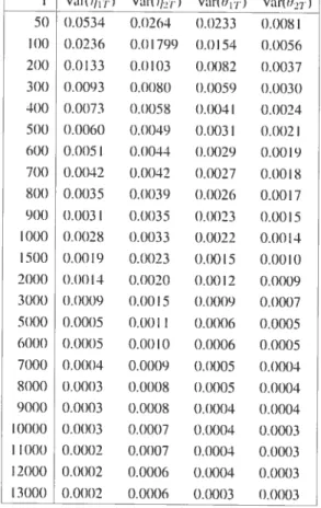
1.1 Single-cquation lincarIV mode!: Monie-Carlovariancesof the new parume

ters ‘)r 55

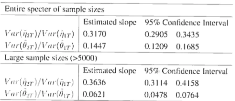
1.2 Sinete—equationlinear IV mode!: Estimation otthe 3coclticientsinthe linear

recression(5.4)und ihe rates of eoIwcrcnce ot the variance scries 56

1.3 Sin2Ie—eqtlation linear IV mode!: Estimationot the•coelhcientsfortheratio

series 56

1.4 CCÀPM: Estimation of the 3 coefficients and the rates ot conveoence ol tue

variance and ratio series forset I 57

1.5 CCAPM Estimation of the coefiicients and the rates of consergenceof ihe

varianceandratio series for set 2 57

1V.! Summary statisiics for the MSCI ofG5 countries over thc period January

1974 io December 995 13!

IV.2 Optima! benchmark c ftr severa! sample sues of the rollingwindow 3! IV.3 Expeeted performances for severa!samplesues of the mlling window 132 IV.4 Expectcd performance tosses whenusing the flasibIe ride instead of its the

orel cal cou nterparl _{I 33}

Table des figures

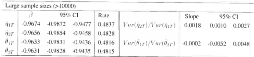
1.1

_{Single-equation linear W model: Logarithm ofthe variance as a firnction of}

thelog-samplesize

₅₈

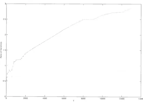
1.2

_{Single-equation linear W model: Ratio ofthe variance of the parameters as a}

function ofthe sample size

₅₉

1.3

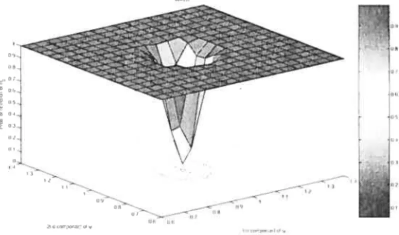
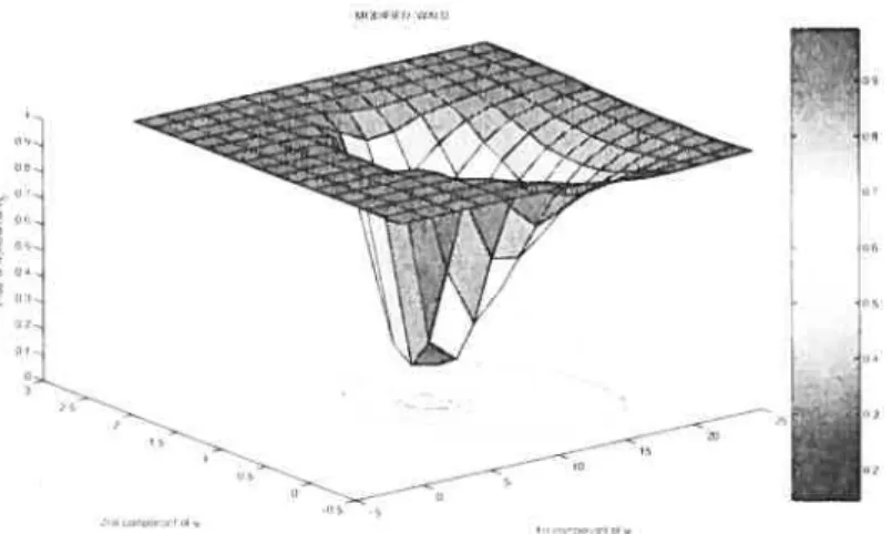
_{CCAPM: Moment restrictions as a function of the parameter values 9}

. .

60

1.4

_{CCAPM: Ratio ofthe variances as a function ofthe sample size}

₆₁

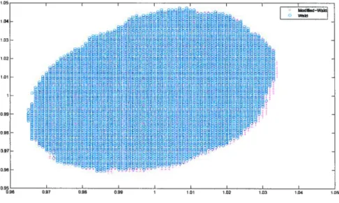
111.1 $5%-Averaged Cotifidence Region when b1 using Modified-Wald and WaId

procedures

₁₀₁

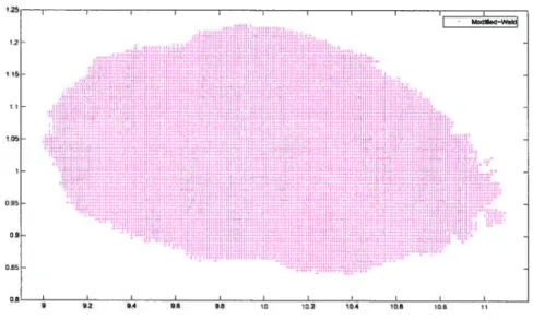
111.2 $5%-Averaged Confidence Region when b=. 1 using Modified-WaM and

WaÏd procedures

₁₀₂

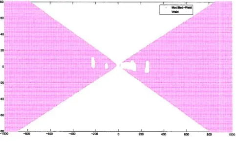
111.3 15%-Averaged Confidence Region when b.1 using Modified-Wald and

Waldprocedures

₁₀₂

111.4 75%-Averaged Confidence Region when b.01 using Modified-Wald and

Waldprocedures

₁₀₃

111.5 1%-Averaged Confidence Region when b=.01 using Modified-Wald and

Waldprocedures

₁₀₃

111.6 Power function when b1 using Modified-Wald procedure

104

111.7 Power function when b=1 using Wald-type procedure

104

111.8 Power function when b.1 using Modified-Wald procedure

105

X

111.9 Power function when b=.1 using Wald-type procedure

.

105

11I.lOPower function when b=.01 using Modified-Waldprocedure

106

111.11 Power fiinction when b.0 1 using Wald-type procedure

106

W 1 Expected performances for several feasible investment niles as a ftmction of

the size ofthe rolling window

134

W2 Expected performances for the p-value investrnent mIes with several bench

marks as a function ofthe size ofthe rolling window

135

Remerciements

Je tiens 10111 d’ahord_{à remercier mon directeur de rccherche. Éric Renault. II} jété présent à

chaque étapeduprocessus : depuis mespremières hesitationsà m’engager (à longterme)en recherche lors de non arrivée à Moiitréal.jusqti’au dernier rebondissement de cette histoire

qui meconduità présent à Vancouver... Sans lui, rien de toutceci ne se serait passé ainsi Un

énormc merci pour les multiples facettes deson sotitien méthodolomque,théorique, moral et financier. Je suis honorée d’avoir PCI évoluer à ses côtés.

Je remercie les lahoratoires de recherche et les institutions qui m’ont accueillie et financée le Centre Interuniversitaire (le Recherche en Économie Quantitative tCIREQ) et le dépar tement d’économie de l’ljnisei-sité de Montréal, le Centre tnlertinisersitaire de Recherche

en Analysedes Organisations (CIRANO). les départements d’économie et de statistiquede UNC-Chapel Hill. Cette thèse a également bénéficiée dcifinancementde bourses de recherche de l’institut de finance MathématiquetIEM2) de \iontréal et dii Conseil de Recherche en SciencesHumaines duCanada tCRSH).

Je remercie les participantsauxconférences, séminaires. grotmpes de travail... pourleurs dis cussions et commentaires.

Enfin, je remercie toutesles personnes qui m’ont épaIllée quandj’en asais besoin : parents, amis. collègues.. la liste est longue. Mercipourvotre présence etvosencouragements:c ‘est aussi grôce à voussij’y suis arrivé.

Introduction générale

Fournirde l’inférence de qualité sur les paramètres «intérêt atoujoursétéune question cen trale en économétrie. Pour ce l’aire, l’approche fréqtientiste se hase sur deux réstiltats es sentiels : la loi des ziands nombres et le théorème de la limite centrale (TLC). Ils assurent respectiement que les vraies valeurs (inconnues) des paramètres sont connues asymptoli cluement. c’est—à—dire cluand la taille de l’échantillon observé tend sers l’inlini, et approchées par des estimateurs asymptotiquernent gaussiens. Sous des hypothèses de régularité standard. il est communément adniis que les résultats précédents sont vérifiés. Dans ces conditions, l’inl’érencc à partir d’une statistique de Wald est très prisée par tes praticiens: on calculetin estimateur de la quantité d’intérêt etson comportement asymptotique est fournit par le TLC

s’en suivent alors les tests et régions de confiance associés. Ces dernières sont construites.

par exemple. en inversant celtestatistique de Wald: celasi2nilie simplement que les valeurs

des paramètres pottr lesquelles le test n’est pas signilïcatifsont collectées. De telles régions sont généralement bornées.

Plus récemment, tin intérêt particulier s’est fait ressentir pocir lournir de l’inférence valide

lorsque _{l’identification des paramètres n’est pitis complètement asstu’ée. Deux situations}

peuvent entraîner tme perte partielle ou totale de l’identification: soit, l’identification est

tout simplement perdueà_{la frontière de l’espace des paramètres soit, lesconditions quias—}

surent l’identification dti modèle font défaut. Dans le premier cas, il est facile d’imaginer une

transformation des paramètres qtii ne serait valide que dans unsous-ensembledel’espace des paramètres d’origine: parexemple. tin ration’est défini que lorsque le dénominateur estnon

nul. Dans le second cas. on peut pensera l’un des cheval de bataille de larecherche empirique

en économie, à savoir I’ instrumentation des ariahles exogènes. Plus précisément,unmodèle

l’on a recours à des variables instrumentales (IV)011instruments potir assurer l’identification

des paramètres du modèle et mener à bien l’inférence statistique. Les instruments sont des sa riahles auxiliaires exogèncs, ou encore non corrélées avec le terme d’erreur, qui doivent être suffisamment pertinentes c’est-à-dire suffisamment bien coiTélées avec les variables expli catives endogènes. Lorsque cette corrélation est faible, l’identification des paramètres n’est

plus complètement assurée.

La perte partielle ou totale d’identitication peut entraîner des comportements asymptotiques inhabitciels chez certaines statistiques de test. Plus généralement. les méthodes d’inférence

standard petivent être invalidées. Pltisicurs articles ont documenté la faible performance des méthodes et approximations asymptotiques cisuclles : entre autres. Nelson et Startz (I Bound. Jacger et Baker (I91)5) _{et Staiger et Stock (1997). Plusieurs pistes (le recherche ont}

alors été envisagées dans la littérature pour fournir desméthodesd’inférence (jables. L’éconemètre peut d’abord envisager une iiodification du cadre de travail en changeant le

scénario asymptotique, afin de potivoirdéris er le comportement asymptotique des statistiques

de test considérées. En d’autres termes, les propriétés d’identification du modèle sont mainte nant liées artificiellement à la taille de l’échantillon. Par exemple. dans le cadre d’un modèle

structurel linéaire à équations simultanées. Staiger et Stock ( 1997) modélisent la corrélation entre les instruments et les s ariahles endogènes comme inversement proportionnelle à la taille

de l’échantillon à la ptussancc 1/2: cette situation est conntie sous le nom d’identification faible, Plus récemment, Hahn et Kuersteincr (2002) considèrent différentes puissances de la

taille de l’échantillon qui caractérisent le degré d’identification: par exemple, l’identification est presque-faible lorsque la puissance est strictement comprise entre O et 1/2.

Une atitre approche consiste à modifier directement les statistiques dc test existantes afin de les rendre robustes aux différents cas d’identification. Par exemple, dans le cadre de la

méthode des moments généralisée (GMM). Kleibergcn (2005) propose le test K ou test du

scoire modifié: l’estmmameur cistmcl dci jacohien espéré est remplacé par un estimateur qin est

asymptotiquemcnt non corrélé avec la moyenne empirique des conditions de moment. Cette modification rend le test robuste aux instruments faibles.

j

dites exactes. Elles ne s’appuient ni sur cine hypothèse d’identification, ni sur la normalité

asymptotiqtie des estimatetirs mais plutôt sur des statistiques pivotales robustes aux pro blèmes d’identification. Citons lapremière d’entreelles, la statistique deAnderson et Robin ou statistiqtte AR (Anderson et Ruhin (949)). Une démarche statistique classiqLte consiste alors à dériver un système d’inférence à partir d’une statistique pivotaI e. Toute la difficulté réside dans l’ohtention de tels pi ots.

Les quatre essais de cette thèse traitent de contextes d’application, en partictilier dans le do maine de l’économie financière, où le point de vue asymptotlqtie traditionnel peut être trom—

pecir. ChaqLie essai propose alors une méthode pouraffinerles approximations asymptotiqtics en présence d’échantillons d’observations c{ui, en praticfue, sont toujoursfinis.

Le premier essai se concentre sur les problèmes d’identification liés à des instruments presqtle faibles. Notre approche consisteàadapter le contexte général de la méthode desmoments gé néralisée IGMM) afin que la Faiblesse des instruments soit en lien direct avec les conditions de moment. Plus précisément, ces dernières _{sont partitionnées suivant l’information statis—} tique qu’elles véhiculentt _{un groupe de conditions de moment standard associé au taux de} convergence hahittiel et cm groupe Faible associé à tin taux plus lent. Les paramètres strtictu rels sont alors estimés de manière usuelle,mais àdes taux de convergence possiblement plcis lents. C’est le cas, en particulier, lorsque le paramètre d’intérêt représente une caractéristique fine dela population qu n’est que faiblement identifiée par les observationsà notre disposi tion : par exemple. la caractérisation des événements rares, le prix des actifs contingents à de

tels événementsou encore le niveau des primes associées à des risques à peine prévisibles. Le decixième essai complète le premier en réalisant une étcide comparative de puissance pour

dccix tests proposés dans la littérature GMM avec instruments (presqtie)-faihles : le test de score classique, valide dans le cadre du premier essai, et le test de Kleihergen (2005) ou score modifié.

L’approche développée dans le_{troisième essai est plus spécifiquement adaptée au cas où le}

défaut d’ identification dti paramètre d’intérêt n’apparaitqu’àla Frontièredu domaine acuorisé des paramètres. Elle considère des régions de confiance potentiellement non bornées dans certaines c’onfigcirations des données d’ohservation, On ne des rait pas être surpris d’obtenir desrégions nonbornées lorsqcie qu’un paramètre n’est pas ou peu identifié eneffet, celles—

ci doivent simplenient être interprétéescomme tin manque d’information disponible dans

l’échantillon pour tournir de l’inférence précise sur ce paramètre.

Enfin, contrastant avec les trois premiers essais qui lestent dans le cadre de la théorie statis tique asymptotique. le quatrième essai adopte plus explicitement tin point de vue décisionnel dans le contexte dci choix de portefeuille. Le risque d’errettr statistique présent dans les mc)— ments estimés est ici considéré simtiltanément avec le risque financier, provenant de l’aléa des rendements : ceci. dans le htit de proposer une gestion intégrée de ces deux risques.Toci tefois, notre solcition passe encore par une approche en termes de test statistique et peLit donc’ être reliée, en ce sens, à la problématique générale de la thèse.

La contribution détaillée de ces quatre essais est à présent développée.

Le premier essai est basé scir un article rédigé conjointement avec Éric Renault. Dans cet es sai, nous ievisitons l’approche d’identification partielle développée par Phillips f1089). lotit en maintenant l’identification complète de tocis les paramètres, mais à des tatix potentielle ment plcis lents. Nocis conservons la normalité asymptotique des estimatetirs GMM, dédciite de l’identification de premier ordre; cependant, le jacohien espéré petit disparaître lorsque la taille de l’échantillon augmente.

À

cet égard, nous sommes dans la lïgnée de la littérature ré cente sur les instruments faibles, qui. sui ant l’approche pionnière de Staiger et Stock t I 997) et de Stock et Wright (2000), capture l’identification faible à partir de conditions de moment empiriques. Toutefois, nous ne spécifions pas a priori le degré d’identification (fort ou faible) des paramètres. Nous considérons que la faiblesse doit être liée plus spécifiqciement acix ins trcirnents, c’est—à—dire atix conditions de moment qui lecir sont associées. Ainsi, la partition fort/faible des paramètres structurels ne petit être atteinte qu’après une rotation adéquate dans l’espace des paramètres.

Par ailleurs, lotit comme Caner (2005 t. nous nous concentrons sur l’identification presque— faible dans laquelle la déficience de rang apparaît à la limite, à un taux picis lent que racine—T. De cette facon, tous les paramètres sont estimés de manière convergente, mais à des tacix pnssihlcment plcis lents qcie d’hahitcide. Il est à noter que la déficience de rang asymptotiqcie considérée garantit toujours des taux de convergence au moins égaux à j’1

pour tous les estimateurs GMM. C’est un contraste important avec l’approche de Stock et Wright (2000):

D

en considérant une déficience asymptotique de rang atteinte au taux racine—T, les estimateurs GMM nesont même pasconvergents. Obtenirdes estimateursGMMconvergents avec des

taux bien_{définis (même s’ils sont potentiellement plus lents qtie la normale) nous permet de} valider les approches de test standard comme Wald ou GMM-LM de Newey et West (1987). Par rapport à Kleihergen (2005). nous n’avons pas besoin de modifier les formules standard pour le test CM.

Il est évident qtic notre approche ne vise pas à capturer des cas sévères d’identification faible qui se proiltiisent même lorsqcie la taille de l’échantillon est très grande (voir Angrist et Krcie

ger (1991)). Toutefois, elle ftcirnitau praticien tIcs procédures d’estimation et d’ inférence qtii

sont valides avec les formules standard, tout en l’avertissant que, dans certaines directions, les tatix de convergence peuvent être plus lents que l’usciel racine—T. Ces résultats sont appli qués _{à un modèle d’équilibre général basé sur le modèle d’évaluation d’actifs CAPM avec} consommation.

Le deuxième essai est basé sur un article rédigé conjointement avec Bric Renault. Il complète le premier essai en réalisant une étude comparative de puissance pour dccix tests proposés dans la littérature GMM avec instruments (presque)-faihles le test de score classique, valide clans le cadre du premier essai, et le test de Kleibergen ou score modifié. Plcis généralement, il s’agit aussi de comparer cIeux approches: d’une part. à t’image dci premier essai, la spécifi cation des problèmes d’identification, ia lecomportement des conditions de moment, offre accès atix procédures de test standard: d’acore part, comme dans Kleihergen (2005), ne faire aucune précision dci cadre d’identification requiert une modification de la statistique du score.

Dans le troisième essai, nous considérons le ratio de paramètres multidimensionnel lorsqtie le dénominateur est proche de la singularité. Nous proposons une nouvelle méthode d’infé rence, la procédcire Modifiecl-Wald. Cette méthode est basée scir la statistique de Wald: il s’agit d’intégrer te contenu informationnel de l’hypothèse nulle d’intérêt dans le calcul de sa métricf oc. Cette correction. toLit_{en préseiant la commodité des calculs, permet l’obtention} de régions de confiance ion bornées lorsque l’identification n’est plcts complètement assurée. Le caractère borné des régions de confiance s’est révélé problématique depcus Dufour (1997). Dans le contexte de la quasi—identification locale (local almost identification), Dufour (1997) fournit des résultats sur la caractérisation des légions de confiance : socis certaines conditions

de régularité, ces régions doivent être non bornées asCC une prohahilite non nulle. En parti— culier. lorstltie l’identification fait défatit, la plupart des ensembles de confiance de type Wald ont_{tin niveau tic conliance nul car ils sont presque sûrement bornés. En comparaison. notre} procédure Modihcd-Wald, aussi attractive dci point de vue computationnel. offre la possibilité d’obtenir des egions de confiance non bornées si nécessaire.

Par aillecirs. lorsque l’identification fait défaut à la frontière de l’espace des paramètres (dans l’esprit de Dufour (1997)). nous montrons que la probabilité d’obtenir tine région de confiance non bornée atteint la borne stipérieure de Dtifour (1997). Lorsque les problèmes d’identification sont (artificiellement) reliés à la taille de l’échantillon (dans l’esprit dti Pit— man drift). cette probabilité dépend dti tatix de convergence vers la non—identification. Par exemple. avec une identification faible (tatix égal à racine—T), cette probabilité est non-ntilie mais pitis petite qtie la borne stipérietire précédente Un exercice de simulation confirme les bonnes propriétés d’inférence de la procédure Modified-Wald par rappoit à Wald avec un ra tio hidimensionnel.

Dans le contexte dii choix de pottefetiille. tin défi important intervient bisque les caiactéris— tiques (inconnties) de la distribution des rendements financiers sont remplacées par des esti més. Ce problème combine donc des difficultés d’ordre statistique à un problème d’économie financière classiqtie consistant à choisir I allocation de fonds optimale. Dans le tluatrième es sai. notis adoptons un point de vue décisionnel afin de développer une règle d’investissement qui incorpore à la fois le risque financier traditionnel et le risque d’estimation. Ce dernier provient directement dti fait que. en pratique. les échantillons sont toujours de taille finie ainsi, les estimés sont-ils tottjoctrs différents de leurs vraies valeurs respectives.

Potir répondre à cette question. nous notis concentrons stir tine mesure de performance dif férente de la littérattire. Nous empruntons atix praticiens et évaluons les différentes alloca tions de fonds à travers leur vraisemblance à battre un niveati de référence. Notre objectif est donc pltis conservateur qti’une maximisation directe de la performance espérée du porte feuille t voir entre autres Markowitz f 1959). Kan et Zhou t2006)). Toutefois. il conesptmd à l’intérêt direct de pltisietirs industries: par exemple. les fonds de pension se doivent de ga rantir un niseau minimal de performance à leurs us estissetirs. Potir tin niseati de référence donné, notis dédttisons une règle U ‘investissement explicite qui incorpore naturellement le risqtic d’estimation de la moyenne et ne dépend d’auctin paramètre dc ntiisance. Ainsi, elle

7

est directement applicable,sans recouriràaucuneétape préalable sous-optimale.

Plus précisément. notre méthode de sélection de portefeuille se hase sur un test unilatéral qui assure que la pertormance du portefeuille est au-dessus d’un niveau de référence donné ensuite, l’allocation optimales’obtient en maximisant la p-valeur associée à ce test. C’est donc en combinant unoutilstatistiquenaturel et valide pour comparer des quantités aléatoires (ici les performances estimées des portefeuilles) à une mestire de performance directement construite à partir des intérêts des praticiens que nous proposonsune règle d’investissement explicite qui intègre directement I’ incertitude du prohlème.

UneétudeMonte-Carlosimple. calibrée à partir de rendements mensuelsdesindices destock

pour les pays dti G5. révèle le bon comportement denotre règle d’investissementen termes de performance espérée hors-échantillon et de stabilité dans letemps par rapport àd’autres règles de la littérature.

Chapitre I

Efficient GMM with Nearly-Weak

Identificationt

9

1

Introduction

ThcCorflcistofleof GMM estiniatiofl iS iiset ol population momentcoiiditions, oltendeduiced Crofl a structural economctric mode!. The limit distributions oC GMtvf estiniators arc dcrived

under_{u central limit theorem (or the moment conditions and u full rank assuluption oC the} expectcd Jacohian. The latter assomptionis not implied hyeconomic theory and many cir

cumstanceswhere itis ailier unjustifiedhavebeen docurnentedin thcliterature (secAndres

and Stock (2005) forurecent sttrxey).

Earlier work on the propertiesoCGMM—hased estimation and inferenccinthe context of rank condition failures includes Phillips (1989) and Sargan (1983). In the contextofa classical linearsimultaneotts equations moUd. Phillipst1989) considers the case oC apcotia/lv identi— /iedstructural equation. He notes tuai, in caseoC rank condition failtire. itis alwayspossible to rotate coordinates in order to isolate estimable linear combinations_{o) the structural pu—}

rameters while the rernaining directions arc completely unidcntitied. Asymptotictheorv ot standard IV estimators in this contexi is then developcd through the general frameworkof

lirnited mixed Gacissian farnily. Thisapproaeh oC par/iaflv ide,iuified models ditfers from Sargan(I983)/irst cmler iuider—ideuti/kaiio,i. While forthe former there is nothing beRveen estimable parameterswithstandard mot—i consistent estirnators and completely uidentified parameters, the latter considcrs that asymptotic identification is stiil otiaranteedbut ii onty’ comes romhigher order ternisinthe Taylor expansionof lirst order optimality conditionsof

GMM: higher order ternis hecomecrucial when(irst order termsvanish. Theyarc rcsponsible

fur sloxer rates oCeonvcrteneeoC GMM estimators like Il and nav lead to non-normal

asymptotic distributions like aCauchy distribution ora mixture of normal distributions. Our contribution in this essay15 to revisit _{an approaeh of partial identification à lu Phillips}

(1989). whule maintaituin, I ikeSariaii(1983), the eomplete identificationoCal parameters.

bLitalpossibly siower rates. Morcover,we remaintruc to asymptotic normalityoC GMM esti Inatorsdeduced mm flrstorder identi(ieation bio s itli an expected Jacohian that _{ma3 vanish}

shen the sample size increases. In this respect. we are in the line oC the recent literatureon weak instruments. which. followingthe seminal approach oCStaigcr und Stock (1997) and

Stock and Wright(2000). capttires weak identilicafionhy drifting population moment condi tions. With respect tothe existing literattire. the contribtition of this essay is as Iollows.

ify a priori which parameters are strongly or wcaklv identiiied. Conforining to the common isdom that eakncss should rather he assigned tu specihc instruments or more generally

tusome specilic moment conditions. we tollow Phillips (1989) to consider that the relevant

partition of ihe sel of structurai parameters between strongIy and weakly identii)cdones can oniy he achievcd after a weli—stiited rotation in thc parameter spacc. In nonlinearsetiings. this change ofhasis dependson unknownstructural parameters andmust itselfhe consistenliy es

timated.

Second. like Caner (2005) (sec also Hahn and Kuersteiner(2002) for the specialcase of

lin-car 2SLS). we fucusun thc case duhhednearh-ncak identijicotio,i.where the driftioiz DGP

introduces a limit rankdeliciency reachedat a rate siower than root- T: this aIlo s consistent estimation of ail parameters. but al rates possihiy siower than usuai. It is then ail ihe more ïmportant to identify the dilfercnt directions in iheparameter space endowed with the ciïfler—

col rates. We consistentiy esiimate these directions viihout assuming that the rates sioer than root—T arc known. We oniy maintain the assomption that the moment conditions re— sponsibie for approximate rank de[iciency have hecn detected. Practicatiy. this either may he thanks tu prior economic knowledge (like market efiiciency responsibie for the weakness of instrcments huiitfrorn past returns in asset pricin_{modeis) or suggested hy a preliminary} study of thc iackoC steepncss uI thc GMM objective fonction around plausible values oC the structurai parameiers. Noie ihat we onivconsidcr asymptotictank deflcienc stich that ail the rates of convergence of GMM estimators. possihly siower than root-T. are at leasi larger than T”’. The Cirst order under-identilication case oC Sargan (i983. producing GM1 esti mators comerging at rates t’’1. can then he seen as a limit case ui our approach. This is in

sharp contras) ith the weakinstrument case à la StockantiWri,lit(2000) where the asymp—

totic rank dehcicncy is reached at u rate as fast as root-T: GMM estimators are nui even consistent. The fuet that ail the GMM estimators are consistent with well-delined rates oC convergence. aiheit possihiy unknown and siower than root-T. ailows us tu val idate standard asymptotic testing approaches like \Vald test or GMM-LM testut Newey and West (19X7). In contrast with Kieihergen (2005). se do not need tu modify the standard formulas ior the LM test. Moreo\er. otir approach is more gencrai ihan Kieihergen (2005) since e expiicitiy take into accotint the possible simuitaneous occurrence, in a gien set oC moment conditions. ut heterogeneocis rates oC cons ergence.

Asfar as technicai tools for asymplutic theory are coneemed. e horrow tc) three rccenl de eiopments in ecunometric theory.

First. as stressed hy Stock and Wriizht (2000). (nearly)—weak identification in nonlinear set tings makes as mptotic theory more invelved than in the linear case hecause theoccurrence of unknown parameters and observations in the moment conditions are flot additively sepa— table. Lees (2004) minimum distanceestimation with heteroizeneous rates ot convergence, aiheit nonlinear. is also kept simple hy this kind ni additive separahility. By contrast, this non—separahility makes. in general. necessary resorting 10a lunctional central limit theorem applied te the GMM objective function viewcdas-Clempirical process indexed hy uitknown parameters.

Second. our approach to Wald testingwith heteregencous rates of convergence must he re lated to the former contribution of Lee (2005). The ke issue isthe folloine: when several directions (te he tested in the parameter space are estimated at slow rates. while some linear combinationsof them may hc cstunated at fttstcr rates. a perverse asymptotic singularity is imroduced and in’alidates the common delta theorem. This situation. rather similar in spirit 10cointegration. leads Lee (2005) te maintain un additional assomption forWald testing. We are able to relax Lee’s (2005) condition und te confirrn that the common Wald test methodol ugy always work. alheit with possihly nonstandard rates of convergence against sequences of local alternatives. The trick is again te consider a convenient rotation in the paramcter space. Note that this issue makes even moie important otir extension of Kleihcrgcn’s (2005) setting to ullow ter dilïerent rates oC convergence simultaneously.

A ihird deht to acknowledge is with respect te Andrews (1994. 1995) MINPIN estiinators’ and te Gagliardini, Gouriérectx and Renault (2005) XMM (Extended Mcthod ot Moments) estimators_{as %ell. Like them. we observe that GMM-like asymptotic variance formulas re} main valid for strongly identified directions hen slowly identihed directions are estimuted al rates faster thanjLt

Rates even slewer than that would imply u perverse contamination oC the estimators oC the standard directions hy poorly idcntified nuisance parameters. In this respect. our approuch should rather he duhhed ncarlv-stmng identification. 0f course, by doing se, we may renounce te capture severe wcak tdenti)ication cases arising even when the sample size is vety large (sec e.gAngrist and Krtieger (1991)). Hewever, ottr appmach pie— vides the empirical economist tth estimation and inference procedtttes that are valid with the standard formulas, while warning her ahotit rates oC convergence in some specific direc tions that may he slower than the standard root—T. Moreover. ihese directions (strong and

MtNPt esiim.ttors are ttetjned as MtNmizi,ie u urjicrion uncuon ttiai ,nghtdepend oit aPretiini,ia,y

weakcan he disentanlcd ancl consistently estitoateci ithottt modiiying the overall rates o

convergence ofthe implied linear combinationsotstructural parameters.

The chapter is organixed as iollows. Section 2 precisely dehnes otir nearly-eak identilica

lion settingandproves consistency ofhoth pointGMM estimators of structural parameters t)

and set estimators. thatarc equivalent b LM-tests of nuit hypotheses O = O. With nearly

weak global identification, consistency ofpoint estimation tests upon an empirical pmcess approach or ihe moment conditions. vhereas set estimation l-ests upon nearly—weak local identification. characieriied in terms of the expeeted Jacohian of the moment conditions. Ont integrated fratuewoi-k restores ihe coherency hetween the two possible points ut view about weak identification, global and local. In section 3. we shov how tu disentangle and

ic) estimate the directions with difterent rates oC convergence. We also prove the asymptotic

normality of well-scnted meut combinations of the structural parameters. The isstie oC Wald

testtn is addressed in section 1 while section5 explicitly relates ont setting tuexamples o

weaL ideniiiicatton well—stLiclied itt_{the literattire. Section 6 is devoted to a couple ot Monte—} Carlo illustrations or two toys tuodels: single—eqtiation meut IV model and CCÀPM.

Ail the proofs and figures ai-e gatbered in the appendix2.

2

Consistent point and set GMM estimators

Ibis section shows that a standard GM M approach wor(shoth for consistent point and set

estimation. the latter thtoLigh u score type test statistic. Typically. ail the componentsofthe

parameters oC interest are simultaneously estimated and iestedwithouto priori knowiedge oC

their heterogenous putters oC identification.

2.1

Nearly-weak global identification

Lei t) he u p—dimensional paratueler vectorwith truc(nnknown) value

oU,

assumed in the in—

tcrior of the compact pararnetcr space The truc pararneter value satisfies the k equations. E [1(oU)]

= t) _(2.1)

Mo’.t ut the iheoretteal reults are Ibtaineci in a note general coniexi iii ateehnical compan(onpaper A iitoineantiRenaultI2007).

13

with

_(.)

_{some lnown functions. We have at mir disposaI a sample of size T, and we can} calculate :, (O) for any valtie of ihe parameler in —3 and for everyt

=

Ï. T.

Standard GMMestimation dehncs its estimator0-as follows:

Definition 2.1. Let Ç-j he

o

sequenceof

sv000ettic

posture clefinite mocloin matrices0/

suce

ii!ich _{coin’erges hi pmbcihilitv toirarcls u positit’e dejinite mcutrLvÏ. A GM,.iesthnator 0} oJ0° is dieu defined as:

or

argiidn

(2r(O)

teheir Qr(0)

iu’iihc1(O)

₌

₊

_{ô1 t 0).} tOc cnipii’ic’aI inca!? of tOc niomenti5’SltïCtiOIlS.

Standard GMM asymptotic theoiy assumes that. for0 0°. o(0) converges in prohahility to\vards Os nonzero expectecl value hecause ni some uniibrin law o) large ntimhers. \Ve consider here a more general sittiation vhere )0) may converge towards cero even for O 0° Ànd we show how this can he interpretedasidentiheation ls5LleS.

Moreprecisely. we imagine thai we have here two groupsofmoment restrictions: une stan dard for which the empirical counterpart converges at the standard (usuat) rate of convergence

VI

and a veakerune for which the empirical counterpart stiti converges but potentially at a stower rate À1. At ihis siaoc. ii is essential to stress ihat identification is goin b he

rnaimained thut through higher order asymptotic developments). More formalty. we have A’

standard moment restrictionssuich that

T [ô(0) —ni

tot]

=

Op(1) (2.3)

and A’1

₍₌

k —A’1) weakermomentrestrictionssuch that

VI

[2Io — n1(0)]

=

01(Ï) svhere À1

=

o(VI)

and À1

L

x (2.4)

with {p’(0) t/,((])]

=

U 0

=

0°.

À1measures the dcgree of wealcnessofthe second group ofmoment restrictions. The corre

sponding component

_t

_{is squeezed tu zct’o and Flint}

_[

_1T)0)]

₌

_{t) for ail 0 E} e. Thus.

such a conteXt. identification is acomhincd propertyofthe fonctions(O) andptO) and the

asymptotic hehavior oC \• The maintained identification assomption is the following:

Assumption I.

Udentification)

(ï) p(.) soconriniiottsfoitc’lïoiifm,no

cotnpoct

pfimntelerspclc’e Cii’ lolo lF’ suclitOut (Q) = t) Q 90

(ii) 19e cinpiricalpmces.v

t

Ji_r(O) obevsaflu cHonul centrc7l Omit theore,n

—Pi

t

Q)

)OT(0)

—fl2(9)

l’(Q)

11901e ili(Q) is u GotissiclnSt0C)tO.SliC pïOCc’SS (fi? iiliIi ineun :eto.

(iii) isu determù,istic sequence of positivereul nirnibers sndttOut À1

À1 x. cind Ititi — O

Followin Stock and Wright (2000), assomption I reinforcesthe standard central limit the orcm written ftrmoment conditions at the trtie value (0 00) _{hy maintaining a functional} centrallimittheorem on thewholeparamctcr set(—j. Stock and Wright (2000) usethis Crame

work b address the weak identification casecorrespondingto À = By contrast. as Hahn

and Kucrsteiner (2002) and Caner t2005),we focushereonncarly-weak identification wherc À5 ocs to tnfinitv albeit slower than

v’T.

Note that the standard stmng identification case corresponds to À5 =

VT.

The ahove functional central limit theorem3 aIIo s _{us to get a}

consistent GMM estimator. evenincase of nearly-wcak identification1.

Theorem 2.1. (Co,tsisiencvof 0)

tI,iderusslonption 1, cmv GMM esli,oolor () like (2.2) ismm’euklv consistent.

Note thai hoasynipioliv normmialiivassunmpimonï.not necear aiibis stars. migemierat.iini iht 0ereplaccd

by some tmhmiiess assomption onmii(). SeeAntoine amid Renamitt 20071.

1A. siressed hy Stock amid Wriht)2000itOcunitornutyiii (i_{providecl hy ihe I unetionat central I iinii iheoremmm}

s criiciat mmi case of nont miicar imonsepaiahleiliOlilOllieoiidiiioiis. itiat j bon tue occurrences ot (9and tue observai ionsinthemoment conditionsarcnom aclctimively separabte. By conirasi. T—latin aitt Knersieincr 201)2) t t inear case) anct Lee 2(104) separable casetdo flot neect tu resomt10fifumictional central t mii theorem.

15

Besides the tact that ail the components _{of the parameter of intcrcst I) are consistently es}

timated, it is worth stressine another di[’tirence with Stock and Wrktht t2000). We do flot assume the oprioriknoIedge of a partition t) (n’ 3’)’. where ‘s is strongly identified and .1 (nearly)-weakly idcntitied. By contrast. nearly-weak identification is produccd hy the rates of eon ergence ol the moment conditions. More precisely. assumption I implies ihat. for the lirst set of moment conclnions. we have tas or standard GMM).

= Ptis t1r(0)

hereas we only have Cor the second set of moment conditions

fIt-O) = Ptim TtO)

It wiIl he shovn that this frameork nesis Stock and Wright 12000). Hahn and Kuersteiner t2002t and Caner t2005t. More precisely. a rotation in the parameter space tsill allow us b _{identity some snongly identihed directions and some others. only nearly t-sseakly identi—} lied. Suhseetion 2.2 helow shows that the ahove rates of convemgence naturally induce rates oC convergence for the Jacohian matrices. This enahies us to encompass tOc framework of Kleihergen (2005).

2.2

Nearly-weak iocal identification

As alreadv explained. we simnuitaneotmsly consider tvo rates ni conergence to characterize ihe asymptotic hehuior oC the sample moments

3(o)

and 10e indciced singtmlarity issues in the sample colmnterparis of the estimating functions p(O). In this respect. ve differ from Sargan f 1083) since we maintain the first—order identification assumption:

Assuniption 2. (fiest—o rUer identification)

(î)p(-) ixconidmiioitslv di/fere,mtiable(711

tue

inlerior of(— denoted asdît)e—)).

(ii) O’ C iisf(E)).

(ni) 111e (1 X s)-inci!ri.v V)t’i O)/U0’] has lis?! cnhunn souk pfdr aU t) E O.

(ii’)

[

]

= pi,

{

T) aT:sӔ

]

T( a, o’’

1

The identification issue is no) raiscd hy rank dchciencv et themoment conditionshic hy the rates et convergence. In other words. the implicit assomption in Klcihergen t2005) (sec the proot et his theorem I page 1122) that Jacohian matrices may have non-standard rates et convergence is made explicit in our framework. Assomptions 2tiv)and (y) are the natural extensions et assomption I en Jacobian matrices. Typically, Kleibergcn (2005) maintains as— sumption 2(v) through ajoint asymptotic normality asstimption on _(O°) and [O7(Ou1_)/Oo’]

(sec his assumption I).

While global identification (assomption I) prov ides a consistent estimator ot f). local identi fication tassumption 2) provides in asyrnptotically consistent confidence set at lecl t I fi) or. equivalentlv. an asymptoticalte consistent test at level n Fr any simple hypothcsis ‘[u : O = _{0. A score test appmach. as defined in Newey and West (1987). does net}

w-soit te the asymptotic distributions cl the estirnators: Theorem 2.2. (Score test)

J7iescore stauisticfor testing [[ O = O ix de/ined as

/ — T

)(2()

ï)(O)_{-i T(U)}

-Ï

30 T 30’

uhere T15o .vicoidatd consiule,I1est jotatc),- o!tueIong—tenu ccit-oricmce matri.x6. Under fI anti as.vlonptions 1 mol 2. L -frt Ou) lias o \2(p)Iioiitdrviribttuion.

In sharp contrast with Klcihergen (2005). ‘se de net need te rnodity the standard score test statistictt)_{replace the Jacohian ot the moment conditions by their projections}017the orthog onal space ot the moment conditions. The reasen tor this rnaintained sirnplicity is that. in our nearly-weakly identilied case.

5/T

2T)

À1 30’

fias a deterministic limit which does no introduce any perverse correlationu. By contrast. in the weakly identificd case considered hy Kleihergen (2005) (or À1 = I). the teletaiit lin7it

ot the sequence et Jacohian niatrices is Gaussian. In this latter case. the limiting behavior Nnte that in general O, niuhi be dit turent train the tille (tuikuowit) valueo) Neparanteter H’’.

‘Note tInt uco,liieltt e%tiinator•5— o!the tong—tetit, c,oariattce natri SH, ut ‘t’Oit cuit Ne huilt in tue %Iandard way t sue in general HaIt (2005))froma prelhitinary _{inetflcieiit HMM estintator (I r ot H. However.} ci tuer Ne nu Il. otie ma siinply chooeHr 0u.

17

of [Li1(0u)/d(ï] is flot indcpendent ot’ the limiting hehavior ot [(OU)] so the lirniting

distributionof the GMM score test statistic depends 00 flUSaflCCparameters (see Stock and Wrfoht (2000)). 0f course. the advantage oC the K-statistic proposed hv Kleihergen (2005) s

b he rohusi in the iirnit case = 1 while. (orus. À1 must aiwuys converge towards inhnity

aiheit possibly very slowly.

h is essential to realize that although the standard score test statisttc lias the cornmon distribution under Oienul),it works rather differently. Basically.

(2.5)

-T

is an asymptotically singtilar matrix sincc

-) it) Î L)/)

(

00)

= r. (I

The proof o) theorem 2.2 shtnvs that the standard formula is actually recovered hy weli—suited matricial scalings ol {OQr(00)/O0’land (2.5). The ultimate cancela0on of these scalings must not conceal that testing parameter in GMM without assuming they are strongly identified

requires a spccilic theory. It isinparticular important to real ice that hoth strong and (nearly)— weak identthcation may show up together in a given set oC moment conditions. Note that this

is immaterial as far as practical formulas for score testing are concerned. Hov evei’. we show

helow that t _{has a dramatic impact on the power against local alternatives7.}

Another difforencewiih Kleiheigen (2005) is that our score test is consisteni in ail directions. Actually. ignoring the kmh case (À1 = 1) oC weak iclentilication aliows us 10 writedown consistent confidence sets and score tests. In ternis oC local alternatives. we get consisteucy

at least at rate \Tthanks

w

the )ollmv ing result: Theorem 2.3. (Raieof c’ometgem’e)

Cuiderassuo,ponsI ond 2(1) îo (iii), ne Iiciie:

—O0 ₌ O

()

Kicihergen t 1t)t)5 coiiider u iinpler setting silice he does toi u) mw loi iwo diflereiti kiiicts o) ideittilica— lion sirong anctsscuki iobe considered siiniiltaneoioly seC the prool oC bis theorein It.In addition. u full tank condition seeiiis ohc’imptic-itlvmaintaineci inKleibcrgen’spinot.

In the ternaining of the essay, wc precisely OCCISon the identification of directions ol local alternatives where consistency is kept al the standard rate

VI.

3

Rates of convergence and asymptotic normality

In this section. we start v 1h a kind of rotation n the parameter space which allows us b disentangle the rates ol convergence. More precisely, sorne special linear combinalions oC O are actually estimated at the standard rate of convergence

VI.

while some others are still cstimated al the slower rate This is formalized by a central lirnit theorem which allows the practitioner to apply the common GMM formula withottt knowing o priori the identification pattern.

3.1

Separation of tue rates of convergence

Weface the followingsituation:

(i)Onlyl equations (de[ined hy[‘t

(.))

have a sample counterpart which converges at the standard rate

VI.

Thesecan he used in a standard way. Unlbitunately. we have in general a reduced tank problem: p, O”)/ifl)’ is not full column rank. lis tank s is stnctly smaller than p and the first set oC equations cannot identify O. Intuitivel>. it can only identify si directionsin the p-dirnensional space oC pararneters.

(ii) The/2 rernainingequations (dcfined byfl2(.)_{) shoutd be used to identify therernaining} 2(=_p— s) directions5. However thisadditional identification cornes al the slower rate .\.

We_{already have the intuition tliat the parameter space is going to he separated mb two sub—} spaces: the Iirst one tdetined through pif.)) collectssi standard diiectionsand the second one tdetined throughfi,).))_{gathers the rernaining (slow) directions. We mw make ihis separation} much more precise h defining a reparametrization. Each of the ahove suhspaces is acittally characterizcd as the range of a full colurnn rank inttrix: respectively the (p s,_{)-rnatrix R} and the (p))— sj)-rnalrix R).

tRecatl ihai. byassulupi oit. oursoioCmomentconditions enablesthe iclemmi deal 10Horthe eimtime vector o) parametersh.

19

Since tt1tcharacterizestheset cii slov directions.it is natural todeline h viathe 11011 space of

[O4

(O0)IdO]. or. inotherwords. es erythinthat isnot identilied in a standard way tthmugh

Pi ( )):

D1

R = 0 (3.))

DO,

-Then these(p — _si) (slow) directions are completedwith the definition ol the remaining

s

directionsas follows:

R = FR R and R,inI [R0]

=p

Then R0 is a nonsingular _{(J’. p)—matrix that can} lie uscd as amatrix of a change of basis in

‘. _{Moreprceisely.ssc dehne}

the new pararneteras,

f

R0]0. that is

O [I? (iii

)

1), i

We will sec in the next subsection that this reparametrication precisely isolates the two rates oC convergence hy dcOnin two subsets ni directions. each oC them associated with a rate ot convergence. The reparametrization also showsthat. in gencral. there is no hope toget standard asymptotic normalityot somecomponents

or

the estirnator_°roC

o°.

The reason is simple: arter a standard expansion oC the lirst-order conditions,0 nowappears as asymptot

icallyequivalentto some lincar transrorrnatitms

or

ijt()_{t ss hich are likely to mix}up the two rates. In otherwords.aIl components of might he contaminated hy the slow rate oC conver gence. Hence themain advantage oCrhe reparametrization is preciselyk) separate these two rates. In section 5f where wecareftilly compare mir theory svith Stock iind Wright (2000), we provide conditions under which some components

or

o

are tby chance) converging at diestandard _{rate. And this is exactly what is assumed n priori hy Stock and Wright (2000)}

when they separate the structural _{parameters into one staitdard-coni’erging group and cime}

sloiier—co,nerç’ingone.

The reparametrization may not he Ceasible in practice since the natrix R° depends on the truc unknossnvalue ol the parameler 0”. However, wecan still dedtice a feasible inference

3.2

Efficient estimation

To be able to get an asymptotic normality resuit on the new set of parameters, we need some

technical assumptions and preliminaiy resuits. More details can be found in the technical

companion paper by Antoine and Renault (2007).

It is worth noting that, albeit with a

mixture

of different rates, the Jacobian

matrix

of moment

conditions has a consistent sample counterpart. Let us first define the following (p, p) block

diagonal scaling matrix AT, where Idr denotes the identity matrix of size r:

AT

t

vId51

O

O

As it cai be seen in the proof oftheorem 2.2, assumption 2 ensures that:

3(O0)

4

J0

with

J°

a:,°)Ro

(3.2)

where J° is the (K, p) block diagonal matrix with its two blocks respectively defined as the

(k, s) matrices [i9p(°)/3O’ R?] for j

=

1, 2. Note that the coexistence of

two

rates of

convergence

()T

and v) implies zero north-east and south-west blocks for J°.

Moreover to derive the asymptotic distribution ofthe GMM estimator

T

(through well-suited

Taylor expansions ofthe first order conditions), the above convergence towards J° needs to

be fulfihled even when the true value

0

is replaced by some preliminaiy consistent estirnator

O. Hence, Taylor expansions must be robust to a )T-consistent estimator, the only rate

guaranteed by theorem 2.3. This situation is rather similar to the one studied in Andrews

(1994) for the so-called MINP1N estimator9. We do not want the slow convergence of some

directions to contaminate the standard convergence of the others (see theorem 3.1 below):

more precisely, we need to ensure that the slow rate

?‘T

does not modify the relative orders

of magnitude ofthe different terms ofthe Taylor expansions. As Andrews (1995 p563) does

for nonparametric estimators, we basically need to assume that our nearly-weakly identified

9MINPIN

_{estimators are estirnators defined as MiNimizing a criterion firnction that might depend on a Pre}

Iiminary Infinite dimensional Nuisance parameter estimator. These nuisance parameters are estimated at siower

rates and one wants to prevent their distributions to contaminate the asymptotic distribution of the parameters

of interest.

21

directions urc estimutcdOa rate (asterthan (Ii 1)•

Inaddition. wè \ant as usttal titorm convergence ot sample Hessian matrices. This eads us tu rnaintain the ftiIIos ingasscunption:

Assumption 3. t 7itvlot evpcutsionx) (I) uni

[]

= x.

VI

(ii)(11(t)) ix twice co,ttiitimttslv difierenticit,le on the interior oJt—9 und ix suc?? ihat:

1T Â( \/i d1

.t°)

j

e’ 1 < k kt fJ1( 0) ancl V I < h <k1

--)t)()3’ — [‘21(0)

iottfrn,nR o,? (I in corne neiglibot-hoidcf (I futr seine

_t

j’.p) ,ncttr,cialfiotctioit fi,k (0)for

9 = 1.2wzd < k <h,.

While common weak identihcition corresponds Le À = 1 mdstwng identitication te

À1

\/7.

_{our approach in the est of the essay is actually a raiher ,iearh-simn one sinec} we assume À strictly hctween T1 and

v’T.’

[p te unusual rates et convergence, we gel n standard asymptotic normuuity resuit forthc newparameleri:

Theoreni 3.1. (AsvinptoticNon,ttilitv)

(j) LIeder osstrntplietts 11e 3, tOc GiclAi estirnator(T defluietl0v2.2) ixsurîttOut: (Or

—

o)

K

(o.

[I°QJ] ‘

_{J°’c)Q)Q5)Jl’}

[J’G.J’]

-‘)

tu)

Under axsmnuplions 1 103, flic’ asvrnptolic taria,lce dlisplavec? in (i) iS ti’hen theGjtvllVtestintcltor ixclefrned tiUha ut’eighirngnuattiv tl7t)euu a consistelilestùnatorof

t) = [S(0’’)]

1[R’1

(t

on)

L

(o.

[.Jutf[S(Ou)] l/fl] I)

wrvjo,e cietatis oit tlte lunl bctwceui Auiclicw(j994. (995tandtitisettine vigie also he Otuticl inÀntoiuie and Renault t 2(107t.

li sorth iem(nciuuig tltat die scoretest deriseci in section 2 iivalici lor\j arbitrarily close b the sveak dent iii cal ioncase.

‘Notelitai e[hcueitc s niplucitly considereci here or the giscnset ol moment restrictions_,(). In section

Note that

‘1?T = [R0]_1T

can be interpreted as a consistent estimator

ofr°

=

[R°1’O°. 0f

course it is not feasibie since R° is unknown. The issue ofplugging in a consistent estimator

of R° wiil be addressed in section 3.4. for the moment, our focus of interest are the implied

rates of convergence for inference about 0. Since

R?]Ï,T

+

R1?2,T

a linear combination a’OT ofthe estimated parameters ofinterest wilI be endowed with a

_v

rate of convergence

of’!1,T

if and only if a’R!

=

D, that is a belongs to the orthogonal space

of the range of Ri?. By

virtue

of equation (3.1) the latter property means that a is spanned by

the columns of the

matrix

[9p (0°)/90]. In other words, a’O is strongly identified if and only

if it is identified by the first set of moment conditions p’(O)

=

O.

As far as inference about 0 is concerned, several practical implications of theorem 3.1

are worth mentioning.

Up to the

unknown

matrix R° and the unknown rate of conver

gence

)p

(which appears in ÀT), a consistent estimator of the asymptotic covariance matrix

(J0i

_{[8(00)1_1}

jo)_1 13

-1 0-1 19T(OT) _laT(ôT)

1

T

AT[R

₁

ae

5T ‘

(3.3)

where

8T

is a standard consistent estimator of the long-term covanance matnx’4. from

theorem 3.1, for large T,

ÀT[R0]_1(T —

00)

behaves like a gaussian random variable with

mean zero and variance (3.3). One may be tempted to deduce that

v”(T —

00)

behaves like

a gaussian random variable with mean O and variance

8(Ô)

‘ T

F)0’

(3.4)

And this would give the feeling that we are back to standard GMM formulas of Hansen

(1982). As far as practical purposes are concemed, this intuition is correct: note

in

particular

that the knowledge of R° is not necessary to perform inference. However, from a theoretical

point of view, this is a bit misleading. first since in general ail components of

‘j

converge

t3This

directly follows from lemma B in the appendix.

14Note that a consistent estimator

of

5’ ofthe Iong-term covariance matrix

S(0°)

can 5e built in the standard

23

asymptolic ‘variance (3.4) s akin te refer te the inverse of an asymptotically singular matrix. Second, ter the saniereason.(3.4) _{is flot an estimator o)’ the standard population matrix}

[)

[S(0°)j ‘t]- (3.5) Te conclude, if inferencc about P is technically moie involved than one may helievc ut lirst sight. it is actuallv ‘verv similar te standard GMM f ‘mulas [‘rom a pure practical point et view. In otherwords. if a practitioncr s net aware of thc specific frarnework with moment conditions associated with several rates of convergence (coming. say. from the use of instru ments of diff’erent qtialities) then she can still provide reliable inference hy using standard GMM formulas. In this respect. we generalize Klcihergcn’s (2005) result that inference can he pcrfoi’med without ci prioriknowledge of the identification sciting. However as already mentioncd in section 2. e are more cneral that Kleiheiiien (2005) since we allow moment conditions te display simultaneously dilf’erent identification patterns’5.

Finally. the standard score test dchned in theorem 2.2 may he complcted hy u classical ovcri dentificat ion test:

Theorem 3.2. (J-lest)

UiuIer assionpilons 1 te3, if Ç)r is u co,isislent estiinutorcf [SU)°)] then

-p

3.3

Orthogonalization of the moment restrictions

Inthis section. _{wc investigate the consequenccs of transforming the moment restrictions to} estimate the standard and slow directions. Since wc deal simultaneously with standard and weaker moment conditions. wc cannot consider any linear comhination et the restrictions.

In _{partietilar. e can only consider transformations prescrving the central limit theorem in}

Àssumption t. and thc liagilc information of thc iveaker moment restrictions. Any valid O_{For suke o)notational}

suuplcliv.we_oiilvcohlsicterintliis esa(iflCpeedor nearlv—weak iclcntiflcaiion.\-t.

The readerImeresiect in work inc w ihan urbit rarynumberoFdi Herein speeds ni ighiusethe geiieral trumen ork nt Antoine und Renau Ii 20)7).