Auteurs:
Authors
:
Hao Dou, Kamel Barkaoui, Hanifa Boucheneb, Xiaoning Jiang et
Shouguang Wang
Date: 2019
Type:
Article de revue / Journal articleRéférence:
Citation
:
Dou, H., Barkaoui, K., Boucheneb, H., Jiang, X. & Wang, S. (2019). Maximal good step graph methods for reducing the generation of the state space. IEEE
Access, 7, p. 155805-155817. doi:10.1109/access.2019.2948986
Document en libre accès dans PolyPublie
Open Access document in PolyPublie URL de PolyPublie:
PolyPublie URL: https://publications.polymtl.ca/4849/
Version: Version officielle de l'éditeur / Published versionRévisé par les pairs / Refereed Conditions d’utilisation:
Terms of Use: CC BY
Document publié chez l’éditeur officiel
Document issued by the official publisher Titre de la revue:
Journal Title: IEEE Access (vol. 7)
Maison d’édition:
Publisher: IEEE
URL officiel:
Official URL: https://doi.org/10.1109/access.2019.2948986
Mention légale: Legal notice:
Ce fichier a été téléchargé à partir de PolyPublie, le dépôt institutionnel de Polytechnique Montréal
This file has been downloaded from PolyPublie, the institutional repository of Polytechnique Montréal
Maximal Good Step Graph Methods for Reducing
the Generation of the State Space
HAO DOU1, KAMEL BARKAOUI 2, HANIFA BOUCHENEB3, XIAONING JIANG1, AND SHOUGUANG WANG 1, (Senior Member, IEEE)
1School of Information and Electronic Engineering, Zhejiang Gongshang University, Hangzhou 310018, China 2Cedric Laboratory, Computer Science Department, Conservatoire National des Arts et Métiers, 75141 Paris, France
3Laboratoire VeriForm, Department of Computer Engineering and Software Engineering, École Polytechnique de Montréal, Montréal, QC H3C 3A7, Canada Corresponding author: Shouguang Wang ([email protected])
This work was supported in part by the Zhejiang Provincial Key Research and Development Program of China under Grant 2018C01084.
ABSTRACT This paper proposes an effective method based on the two main partial order techniques which are persistent sets and covering step graph techniques, to deal with the state explosion problem. First, we introduce a new definition of sound steps, the firing of which enables to extremely reduce the state space. Then, we propose a weaker sufficient condition about how to find the set of sound steps at each current marking. Next, we illustrate the relation between maximal sound steps and persistent sets, and propose a concept of good steps. Based on the maximal sound steps and good steps, a construction algorithm for generating a maximal good step graph (MGSG) of a Petri net (PN) is established. This algorithm first computes the maximal good step at each marking if there exists one, otherwise maximal sound steps are fired at the marking. Furthermore, we have proven that an MGSG can effectively preserve deadlocks of a Petri net. Finally, the change performance evaluation is made to demonstrate the superiority of our proposed method, compared with other related partial order techniques.
INDEX TERMS Petri nets, state explosion problem, covering step graph methods, persistent sets.
I. INTRODUCTION
Concurrent systems [1]–[3] are composed of several subsys-tems operating in parallel and they are especially difficult to be designed or analyzed in the real world [4]–[9]. Thus, the design correctness of concurrent systems needs to be checked via the verification.
The state space exploration method [10]–[14] is one of the most widely used techniques for the verification of finite-state concurrent systems. However, there exists an obstacle in the application of this technique, which is the state-space explosion. This problem is mainly caused by the interleaving semantics of concurrent systems, i.e., all firing orders of concurrent transitions are explored exhaustively, during the application of such technique. Actually, many researchers have studied strategies fighting for this problem and several different techniques are proposed such as compositional ver-ification, symmetric reduction, abstraction and partial order reduction.
The associate editor coordinating the review of this manuscript and approving it for publication was Zhiwu Li .
The partial order reduction [38]–[55] has been proven to be the most successful strategy for alleviating the state-space explosion in practice [54]. It can utilize the indepen-dence of concurrent execution to eliminate some interme-diate states [56]–[57]. More precisely, there is no need to explore all interleaving semantics possessing identical concurrent execution, when analyzing properties of interest (deadlock freeness [17]–[27], reachability [28]–[32], live-ness [33]–[37], or linear properties [38]).Note that partial order reduction techniques, such as stubborn sets [46]–[48], sleep sets [43], ample sets [49]–[50], persistent sets [42]–[43] and covering step graphs [52], preserve deadlocks of Petri nets (PNs) [15]–[16] at least.
The covering step graph methods explore all the transitions of the state space and concurrent ones are put together to constitute an atomic step. They aim to reduce the depth of the marking graph while the purpose of the persistent sets is to reduce its breadth. The persistent sets are intro-duced in [42], [43], which are particular stubborn sets. Dif-ferent from the covering steps, persistent sets only explore enabled transitions at each marking. To make full advantage of both methods, Ribet et al. [53] present a persistent step
graph (PSG) which can both improve persistent sets and covering step graph methods, and reduce the state space from its breadth and depth. More importantly, it has been proven that the PSG preserves the deadlocks of Petri nets. In order to further reduce the state space, Barkaoui et al. [54] propose the maximal persistent step graph (MPSG) method and intro-duce a new definition of weak-persistent sets. Combining the weak-persistent sets with covering steps, the MPSG achieves a more significant reduction of the state space, compared with the PSG.
In this work, according to the definition of covering step graphs introduced in [52] we first propose a new definition of sound steps, which is an extension of covering steps. Then, from a practical point of view, a weaker sufficient condition about how to build the set of sound steps at each marking is introduced. Based on this condition, we can compute the set of maximal sound steps at each marking more intuitively and quickly. Next, we propose a definition of good steps, combing maximal sound steps and persistent sets. Due to the proposed good steps and maximal sound steps, a maximal good step graph (MGSG) is constructed, which significantly reduces the state space compared with other related partial order reduction methods. In addition, the MGSG preserves deadlock markings of Petri nets. The major contributions of this work are listed as follows:
1) We propose a new definition of sound steps, based on a better understanding of the concurrent and conflict relations between transitions of a step. Thus, the firing of a sound step at each marking enables to extremely reduce the state space;
2) Based on the definition of sound steps, we propose a weaker sufficient condition about how to find the set of sound step at each marking, which is of practical significance;
3) Combining the persistent sets and sound steps, a new definition of good steps is introduced, which plays an important role in computing the maximal good step graph (MGSG)
4) The generated maximal good step graph permits to pre-serve the deadlocks of a Petri net.
The rest of this paper is structured as follows: Basic knowl-edge used throughout this paper is introduced in Section II and Section III presents the definition of persistent sets, and followed by some previous partial order reduction methods, which are the basic of our proposed method. Section IV first introduces the new definition of sound steps, then proposes a weaker sufficient condition for sound steps, next presents the concept of good steps and exhibits the construction algorithm of the MGSG, finally proves that the MGSG preserves the deadlocks of Petri nets. Section V compares our proposed technique with other related partial order reduction meth-ods and shows the experimental results to demonstrate the superiority of our method. Finally, Section VI concludes this work.
II. PRELIMINARIES
In the following discussion, E∗ represents the set of all sequences constituted by elements of E (i.e., including an empty sequence ε) and E+ denotes the set of sequences withoutε, such that E∗:= {ε} ∪ E+. For instance, E = {e, f}, E∗= {ε, e, f , ee, ef, fe, ff , . . .} and E+= {e, f , ee, ef, fe, ff, . . .}.
Fundamental notations related to Petri nets and partial order methods are introduced in this section. A reader may consult more details in [15]–[16], [53]–[54].
A generalized Petri Net (PN) is a 4-tuple N = (P, T , F , W ), where P and T are denoted as non-empty, finite, and disjoint sets. P characterizes a set of places and T describes a set of transitions. There is a flow relation F , which is represented by directed arcs from places to transitions or from transitions to places. W : (P × T )∪ (T × P) → N = {0, 1, 2, . . .} is a mapping that assigns a weight to an arc. It satisfies that W (x, y)> 0 if (x, y) > F, and W (x, y) = 0, otherwise, where x, y ∈ P ∪ T. If ∀ (x, y) ∈ F , W (x, y) = 1, this net is called an ordinary Petri net, denoted by a 3-tuple N = (P, T , F ). Given a node x ∈ P ∪ T , the pre-set of x is denoted by•x, where•x = {y ∈ P ∪ T |(y, x) ∈ F }, and the post-set of x is expressed as x•={y ∈ P ∪ T | (x, y) ∈ F }. We can extend this notation to a set of nodes, i.e., ∀X ⊆ P∪T ,•X = ∪x∈X•x
and X•= ∪x∈Xx•.
A marking (or state) M of N is a mapping from P to N, where N represents nonnegative integers. For the sake of convenience, the multi-set symbolP
p∈PM(p)p is utilized to
denote vector M , where M (p) indicates the number of tokens in p at M . For example, M = [3, 2, 1, 2]T is denoted by
M =3p1+2p2+ p3+2p4. A place p is marked by M if
M(p) > 0. We define (N, M0) as a Petri net system with its
initial marking M0.
The transition t ∈ T is enabled at a marking M , denoted by M [ti, if ∀p ∈•t, M (p) ≥ W (p, t). The firing of t at M yields a marking M0, i.e., ∀p ∈•t, M0(p) = M (p) − W (p, t) + W (t, p), which is denoted as M [tiM0. The marking M0 is called an immediately reachable marking from M . The set of all transitions enabled at M is denoted by En(M ) = {t ∈ T |∀p ∈•t, M (p) ≥ W (p, t)}. The sequenceσ = t1t2. . . tn∈
T∗is enabled at M , denoted as M [σi, if there exists a series of markings M1, M2, . . . , Mn−1such that M [t1iM1∧M1[t2iM2∧
. . . ∧ Mn−1[tni. A marking M00is said to be reachable from
Mif the firing of a sequenceσ ∈ T∗at M yields the marking M00, which is indicated as M [σiM00. We use the notation R(N ,
M) to denote the set of all markings reachable from M of N . A non-empty subset of transitions is said to be a stepτ of N (τ ⊆ T ) if the firing of transitions in this step is simultaneously and atomically at a marking M of N . To con-sider a firing step from an interleaving semantic standpoint, it can be viewed as an abstraction of all sequences of its transitions. For example, a step τ = {t, t0, t00} hides six sequences of its transitions: tt0t00, tt00t0, t0tt00, t0t00t, t00tt0, and t00t0t. A stepτ is enabled at a marking M, denoted as M [τi, if ∀p ∈ •τ, M(p) ≥ Pt∈τW(p, t), which means that there
are enough tokens allowing transitions within the step to fire concurrently. Firing a stepτ yields a marking M0such that ∀p ∈•τ, M0(p) = M (p) +P
t∈τ(W (t, p) − W (p, t)), which
is denoted by M [τiM0. A marking M00is said to be reachable in multiple ways from M if there exists an enabled transition t at M and after the firing of t, there exists a sequenceσ, a step τ and two intermediate markings M1, M2such that M [tiM1
[σi M2[τiM00, which is indicated as M [tσ τiM00. Note that
as long as the enabled conditions are satisfied, the firing order of a transition t, a sequenceσ, and a step τ is arbitrary, i.e., M [tσ τiM00, M [tτσiM00, M [σtτiM00, etc. We use EnStep(M ) to denote the set of all enabled steps at M . Given an enabled stepτ ∈EnStep(M), τ is maximal at M if (τ0 ∈ EnStep(M ) such thatτ ⊂ τ0. We denote by Step(T ) the set of all steps of a PN N .
Transitions t1and t2are in structural conflict, denoted by
t1⊥t2, if•t1∩•t2 6= Ø. Transitions t1and t2are symmetric
structural conflict with each other, denoted as t1⊥st2, if t1⊥t2,
and•t1∩•t2∩ t1• =•t1∩•t2∩ t2•. Two transitions t1and
t2are in conflict, denoted as t1# t2if the firing of t1(or t2)
may disable the transition t2(or t1) at a marking M where t2
(or t1) should have been enabled. We use CFS(t) = {t2 ∈
T |t1# t2} to denote the set of transitions in conflict with t1.
The transitive closure of conflict relation is weak conflict. Transitions t1and t2are in weak conflict, which is denoted
by t1[#] t2. The set of transitions in weak conflict with t1is
denoted as [CFS](t) = {t2 ∈ T |t1[#]t2}. Notice that t ∈ T
and CFS (t) ⊆ [CFS](t).
Two sequences of transitions σ and σ0 are equivalent, denoted as σ ≡ σ0 if they are the same or each one can
be obtained from the other by successive permutations of transitions. Let M be a reachable marking. ∀M0 ∈ R(N , M), equivalent sequencesσ and σ0from M lead to the same marking M0, i.e., M [σiM0and M [σ0iM0, ifσ ≡ σ0. We use [σ] to denote the set of transitions contained in a sequence σ. A reachability graph RG of N is a finite and labeled directed graph, denoted by RG = (R(N , M0), →, T , M0),
where → is a directed edge from a marking M to another reachable marking M0, where M , M0 ∈ R(N , M0), and it is
labeled by a transition t of T. A covering step graph CSG of Nis defined by CSG = (RS(N , M0), →, Step(T ), M0), where
RS(N , M0) ⊆ R(N , M0) is a subset of reachable markings, and
→is labeled by an enabled stepτ ∈ Step(T ) at each marking M ∈ RS(N , M0).
Given a PN (N , M0), a transition t ∈ T is live at the initial
marking M0 if ∀M ∈ R(N , M0), ∃M0 ∈ R(N , M ), M0[ti.
This net (N , M0) is live if each transition t of N is live at
M0. The reverse case is that a transition t is dead at M0 if
∀M ∈ R(N , M0),¬M[ti. (N , M0) is dead if @t ∈ T , M0[ti.
A marking M ∈ R(N , M0) is a deadlock marking if ∀t ∈ T , ¬M [ti, which can be described as En(M ) = Ø. The net (N ,
M0) is called deadlock-free (i.e., not-dead or weak-live) if
∀M ∈ R(N , M0), ∃t ∈ T , M [ti. A place p ∈ P is k-bounded
if given M ∈ R(N , M0), ∃k ∈ N+: M (p) ≤ k, where N+
represents positive integers. The PN (N , M0) is a k-bounded
net if each place p of N is k-bounded. Note that the PN (N , M0) is said to be safe iff k = 1.
In this paper, we only focus on the ordinary Petri net N =(P, T , F , M0).
III. PARTIAL ORDER METHODS
In this section, we introduce the persistent sets and covering step graph methods, and their combination.
A. PERSISTENT SETS
At each marking, persistent sets only contain enabled tran-sitions. Note that each transition of a persistent set can not be disabled, by the firing of other transitions not in the same persistent set [43], [53]. In general, the exploration of persistent sets preserves at least deadlocks of Petri nets.
The persistent sets proposed by [43], [53] are called strong-persistent sets. In [54], the authors introduce weak-strong-persistent sets with weaker conditions inspired from stubborn sets of [46]. In the following discussion, the persistent sets used throughout this paper are strong-persistent sets.
Definition 1 [54]:Let M be a marking andµ ⊆ En(M)
a subset of enabled transitions. Formally, the subsetµ is a persistent set of M if all the following conditions are satisfied:
1) En(M ) 6= Ø ⇔µ 6= Ø;
2) ∀t ∈µ, ∀ω ∈ (T − µ)+, M [ωi ⇒ M[ωti; 3) ∀t ∈µ, ∀ω ∈ (T − µ)+, M [ωti ⇒ M[tωi.
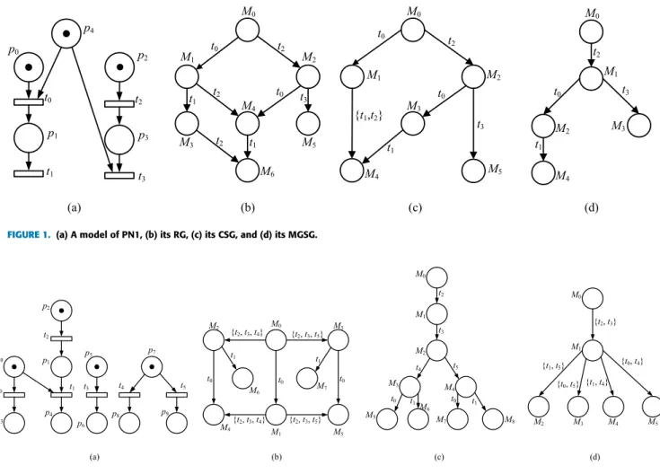
Condition 1) means that there exists no persistent set at M iff M is a deadlock marking. Condition 2) ensures that after the firing of transitions not inµ at M, any transition t of µ can be fired. Condition 3) states that if the firing of any sequence ω, which is composed of transitions not in µ, does not disable any transition t ofµ, and then the firing of t will not disable ω. Consider the PN1 in Fig. 1(a). The set of enabled transi-tions at M0is En(M0) = {t0, t2}. Letµ1 = {t0} be a subset
of En(M0). It is not a persistent set since t0is disabled by the
firing of a sequence t2t3, i.e., M0[t2t3ibut¬M0[t2t3t0i. For
the same PN1, the setµ2= {t2} is persistent as conditions 1,
2 and 3 hold for t2.
B. STEP GRAPHS COMBINED WITH PERSISTENT SETS Covering step graphs are proposed in [52]. In a covering step graph, all transitions are visited and concurrent ones are put together to constitute a step. The firing of transitions in a step is simultaneously. The aim of step graph methods is to achieve more reduction of the state space from path depths, and preserve certain global reachability properties such as deadlocks. For example, consider the model PN2 depicted in Fig. 2(a). There exist two steps at the initial marking M0,
τ1 = {t0, t2, t3, t4} and τ2 = {t0, t2, t3, t5}. However,
the firing ofτ1or τ2 may disable t1that should have been
enabled at a marking M1, where M0[t2iM1. Thus, t0cannot be
fired together with t2since some deadlock markings may not
be preserved if they are fired simultaneously. The covering step graph (CSG) is shown in Fig. 2(b) and firing steps at
FIGURE 1. (a) A model of PN1, (b) its RG, (c) its CSG, and (d) its MGSG.
FIGURE 2. (a) A model of PN2, (b) its CSG, (c) its PG, and (d) its MGSG.
M0are τ1 = {t2, t3, t4},τ2 = {t2, t3, t5} and τ3 = {t0}.
Specially, the covering step graph preserves deadlocks of PN2 and reduces the state space from path depths.
Different from covering step graphs, persistent graphs (PG) are to reduce the width of the state space. At each marking, only the enabled transitions of a persistent set are visited and fired individually. For instance, consider the same PN2, the set of enabled transitions at M0is En(M0) = {t0, t2, t3,
t4, t5} and there are three persistent sets at M0:µ1= {t0, t2},
µ2= {t3} andµ3= {t4, t5}. The firing of a transition within
different persistent sets may yield different persistent graphs. A minimal persistent graph of PN2 is shown in Fig. 2(c).
To make full use of the advantages of covering step graphs and persistent sets, a hybrid method is proposed in [42]. The main idea of its generation algorithm is to compute persistent sets at each marking firstly, and then determine which transi-tions in different sets can be combined together as a step. The combination of both methods allows reducing the state space from path depths and the width, and preserves the deadlocks of PNs. As an example, consider the PN2. For the persistent sets {t0, t2}, {t3} and {t4, t5} of the initial marking M0, we can
build various steps such as {t0, t3, t4}, {t0, t3, t5}, {t2, t3, t4},
{t2, t3, t5}, and {t2, t3}. These steps are so-called persistent
steps and the firing of different one at M0may lead to different
persistent step graphs. According to the algorithm proposed in [41], the maximally reduced persistent step graph (PSG) is depicted in Fig. 2(d).
For these reduced state graphs, some intermediate mark-ings are abstracted and all key markmark-ings are preserved. The key markings of a PN can be utilized to explore certain global reachability properties such as deadlocks of a PN.
IV. MAXIMAL GOOD STEP METHODS A. SOUND STEP SETS
Definition 2:Let M be a reachable marking of a PN N = (P,
T, F , M0),τ an enabled step at M and t ∈ τ. The transition
t is sound at M w.r.tτ if conditions 1) and 2) hold for all t0∈τ− {t}: 1) ∀σ ∈ (T −{t})+, (M [t0σ i ∧¬M[t0σti) ⇒ a) ∃σ∗∈(T − {t})+, M [t0σ σ∗ti∨ b) ∃t1 ∈En(M ) − τ, ∃σ1 ∈ (T −{t})∗, (t1σ1 ≡ σ ∧ M[t1t0σ1i) 2) ∀σ ∈ (T −{t})+, M [t0σti ⇒ ∃σ0 ∈ (T −{t})+, (σ ≡ σ0∧ M[tt0σ0i)
The stepτ is sound at M if its transitions are all sound at M with respect toτ. We use the notation SS(M) to indicate the set of all sound steps at a marking M of a PN N .
For a sound transition t w.r.t.τ at M, Condition a) shows that t can be re-enabled after the firing of a sequence starting with certain transitions of the same step τ and Condition b) means that the disableness of t cannot be caused by other transitions of the same stepτ; and Condition 2) states that if a sequence t0σt is firable from M, then there must exist an equivalent sequence tt0σ0 that is also firable from M . Specifically, in a case where t is disabled by an enabled sequence t0σ , i.e., M[t0σi ∧¬M[t0σti, if the firing of t0σ satisfies a certain condition (i.e., Condition a) or b)), then we can be sure that t is sound at M . Condition a) represents that the sequence t0σt that is used to be not enabled at M can
be fired s.t. M [t0σ σ∗ti. Intuitively, it means that if a
transi-tion t is disabled after the firing of other transitransi-tions within the same step τ, i.e.,¬M[t0σti, then the sound transition t can be re-enabled after the firing of other sequences, i.e., M[t0σ σ∗ti. Condition b) shows that the sequence t0σ has an equivalent and enabled sequence at M that starts with a certain transition outsideτ s.t. t0σ ≡ t1t0σ1and M [t1t0σ1i,
which means that the sequence t0σ leading to the disableness of t can be fired at M in another order and then the firing of t cannot be affected by t0σ. Note that expressions such as ‘‘t1σ1 ≡ σ’’, ‘‘M[t1t0σ1i’’, ‘‘σ ≡ σ0’’, and ‘‘M [tt0σ0i’’
can be considered as boolean expressions. More specifically, the value of ‘‘t1σ1≡σ’’ is 1 if the sequence t1σ1is equivalent
toσ , otherwise its value is 0.
It is obvious that if |τ| = 1 then τ is a sound step at M. Indeed, in such a case t0 ∈ Ø, the sequence t0σ is not
enabled at M , i.e.,¬M[t0σ i, since for an enabled sequence, the first transition must belong to En(M ). Hence, it follows that Conditions 1) and 2) are satisfied.
Example 1:As an example of a sound step, consider the
PN4 in Fig. 4(a). The enabled stepτ = {t1, t2, t3} of the initial
marking M0= p1+ p2+ p3is sound since it satisfies
Defi-nition 2. Specifically, an enabled stepτ1 = {t2, t3} of M0is
also sound. For instance, Condition 1) is satisfied for t2w.r.t.
τ1 since M0[t2t4i and ¬M0[t2t4t3i, there exists an enabled
transition t1 such that M0[t2t4t1t3i; and Condition 2) also
holds for t2 since M0[t2t4t1t3i, there exists a sequence t1t4
equivalent with t4t1s.t. M0[t3t2t1t4i. The set of all sound steps
at M0of the PN4 is SS(M0) = {{t1}, {t2}, {t3}, {t1, t2}, {t1,
t3}, {t2, t3}, {t1, t2, t3}}. As another example of a sound step,
consider the PN5 shown in Fig. 6. The enabled stepτ = {t1,
t4, t5} is sound at the initial marking M0= p1+ p4+p5since
Conditions 1) and 2) hold for each transition ofτ. The set of all sound steps at M0is SS(M0) = {{t1}, {t4}, {t5}, {t1, t4},
{t1, t5}, {t4, t5}, {t1, t4, t5}}. Taking a sound stepτ1 = {t4,
t5} for an example, we can see that Condition 1) is satisfied
for t5since M0[t5t6iand¬M0[t5t6t4i, there exists a sequence
t1t2t3such that M0[t5t6t1t2t3t4i; and Condition (2) also holds
for t5since M0[t5t6t1t2t3t4i, there exists a sequence t1t2t3t6
equivalent with t6t1t2t3s.t. M0[t4t5t1t2t3t6i. As an example of
a non-sound step, consider the PN1 depicted in Fig. 1(a). The
enabled step {t0, t2} of the initial marking M0 = p0+ p2+
p4 is not sound since Condition 1) does not hold for t2:
M0[t2t3iand¬M0[t2t3t0i, but we have neither a) nor b) due to
there exists no sequenceσ∗∈(T −{t})+s.t. M [t2t3σ∗t0iand ¬M
0[t3t2i. Thus, the set of sound steps at M0of the PN1 is
SS(M0) = {{t0}, {t2}}. Another example of a non-sound step
is PN3 shown in Fig. 3(a). An enabled stepτ1 = {t0, t2} of
the initial marking M0 = p0+ p1+ p2+ p4is not sound as
Condition (1) does not hold for t2. Intuitively, the sequence
t2t3t1 is firable at M0 but t2t3t1t0 is not firable at M0, i.e.,
M0[t2t3t1i ∧¬M0[t2t3t1t0i, and we have neither a) nor b) as
there exists no sequenceσ∗ ∈(T − {t})+s.t. M [t2t3t1σ∗t0i
and¬M0[t1t2t3i. For the same PN3, the enabled stepτ2= {t1,
t2} of M0is also not sound as it does not satisfy Condition(2)
since M0[t2t3t1ibut¬M0[t1t2t3i. Hence, the set of sound steps
at M0of the PN3 is SS(M0) = {{t1}, {t2}, {t3}}.
B. PROBLEMS STATEMENT
We first propose two problems used in the following section.
Problem 1:Given a PN N and its initial marking M0, how
to find the set of sound steps at each reachable marking from a practical point of view?
Essentially, The answer of Problem 1 corresponds to a weaker sufficient condition for sound steps. From a practical point of view, we need to explain clearly the way about how to build the set of sound steps at each marking. Hence, we ana-lyze how to determine which transitions can be constitute as a sound step at each marking, from the aspect of a net structure. Let M be a marking of N andτ ⊆ En(M) an enabled step at M withτ = {t, t0} (i.e., |τ| = 2). If t and t0satisfy the following conditions, we can know that the stepτ at M is a sound step. In other words, we can find which step is sound at M according to the following conditions:
1) Transitions t and t0are not conflict with each other. Actually, if t are in conflict with t0, then transitions t and t0can not be fired together at M .
2) There is a transitionµ that is conflict with t. We can distinguish three cases for the type ofµ.
a) The transitionµ is not enabled at M and there exists a sequenceσ ∈ T∗s.t. M [t0σiM0∧ M0[µi. We need to
determine whether there exists an enabled transition t∗, s.t. t∗ ∈ En(M ) −τ and the preset p∗ of t∗ can give its token to the common place p of t and µ. If the transition t∗and the place p∗satisfy the above condition, then t and t0may be constituted as a sound step at M .
b) The transitionµ is not enabled at M and the firing of t0can not yield a marking M0s.t. M0[µi.
c) The transition µ is enabled at M. We continue to distinguish this case into two categories:
i. There is a disabled transitionν that is in symmet-ric structural conflict withµ;
ii. There is a disabled transitionν conflict with µ and the firing of t0can not yield M0s.t. M0[νi.
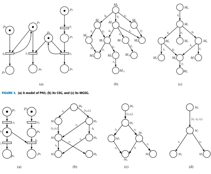
FIGURE 3. (a) A model of PN3, (b) its CSG, and (c) its MGSG.
FIGURE 4. (a) A model of PN4, (b) its CSG, (c) its MPSG, and (d) its MGSG.
If two transitions of a step τ at M satisfies the above conditions, we can say that τ is sound at M. For instance, τ = {t4, t5} of the PN5 in Fig. 6 is a sound step at the initial
marking M0since t4is conflict with t6and M0[t5i M0∧M0[t6i.
We can find that there exists an enabled transition t1outside
the stepτ and the preset p1of t1gives its token to the common
place p4of t4 and t6. Thus, {t4, t5} is a sound step at M0.
As another example of a sound step, consider the same PN5. The stepτ = {t1, t4} is also sound at M0since t4is conflict
with t6 and there does not exist a sequence σ ∈ T∗ s.t.
M0[t1σiM0 ∧ M0[t6i. As an example of a non-sound step,
consider the PN3 shown in Fig. 3(a). The stepτ = {t1, t2}
is not sound at the initial marking M0 since t1 is conflict
with t3and M0[t2i M0∧ M0[t3i. However, we cannot find an
enabled transition t∗s.t. the preset p∗of t∗can give its token to the common place p4of t1and t3. As another example of
a non-sound step, consider the same PN3. The stepτ = {t0,
t2} is also not sound at M0since t0is conflict with an enabled
transition t1of M0and t1is conflict with another transition t3
which is not enabled at M0. However, t3is not in symmetric
structural conflict with t1 and the firing of t2 can lead to a
marking M0s.t. M0[t3i.
Problem 2:Given a PN N and a reachable marking M , how
to determine a stepτ with |τ| > 2 is a sound step at M? In terms of Problem 1, we know how to find a sound step τ at each marking with |τ| = 2. It is obvious that τ is always a sound step at M with |τ| = 1 according to Definition 2. As for a stepτ at M with |τ| > 2, we first find all transitions ofτ, and then estimate whether two arbitrary transitions can be fired together as a sound step according to Problem 1. If so, the stepτ containing these transitions with a bigger range is sound at M . For example, the stepτ = {t1, t4, t5} is sound at
M0of the PN5 in Fig. 6 since {t1, t4}, {t4, t5} and {t1, t5} are
all sound at M0.
C. A CONSTRUCTION ALGORITHM FOR AN MGSG
In this section, we first introduce a function named
Max-SoundStepto compute the set of all maximal sound steps at
each marking of a PN N . Then, we present a relation between maximal sound steps and persistent sets, and followed by the
notion of good steps that combine sound steps with persistent sets. Afterwards, a construction algorithm for a maximal good step graph (MGSG) is established and we prove that such a graph preserves deadlocks of a PN.
We exhibit Function MaxSoundStep in the following. Let IsSoundbe a decision function defined by: given a reachable marking M of a PN N and an enabled stepτ of M, IsSound(M, τ) = false, if transitions of τ at M do not satisfy the sufficient conditions of Problem 1. In other words, IsSound(M ,τ) = true signifies that τ is sound at M. A sound step τ is the maximal one at M , if there does not exist another sound step τ0at M s.t.τ ⊂ τ0. Note that Function MaxSoundStep will be
used in the construction algorithm for an MGSG.
Function MSS = MaxSoundStep(M ) Input: A marking M of a PN N ;
Output: A set MSS of all maximal sound steps at M ;
1. MSS = Ø; 2. MS = {En(M )}; 3. S = Ø; 4. while (∃τ ∈ MS s.t.¬IsSound(M ,τ)) do 5. MS = MS −τ; 6. S = {τ0|∀t ∈τ, τ0=τ − {t}}; 7. for (eachµ ∈ S s.t. ∀π ∈ MS, µ 6⊂ π) do 8. MS = MS ∪{µ}; 9. end for 10. end while 11. MSS == MS; 12. Output: MSS.
In brief, Function MaxSoundStep is executed as follows: First, let MS be the set of all enabled transitions set at a marking M , i.e., MS = {En(M )}. Then, a step τ of MS, which is not sound according to Problem 1, is deleted. After deleting the stepτ, we define a symbol S to compute the set of all maximal subsets ofτ. Each step µ of S, which does not belong to a stepπ of the deleted MS, is added to the set MS to combine the new set of maximal steps. By repeating the above process, the set of all maximal sound steps at a marking M is computed.
Example 2:Consider the PN3 shown in Fig. 3(a) and its
initial marking M0= p0+ p1+ p2+ p4. In terms of Function
MaxSoundStep, MS = {En(M0)} = {{t0, t1, t2}} andτ = {t0,
t1, t2}. By Definition 2, it is obvious thatτ is not sound at M0
and thus is deleted from MS. The set MS is then replaced with
MS = {Ø}. The set S of all maximal steps inτ is computed
s.t. S = {{t0, t1}, {t1, t2}, {t0, t2}} and MS is replaced with
MS = {{t0, t1}, {t1, t2}, {t0, t2}} since each step of S does
not belong to {Ø}. We can see that these steps {t0, t1}, {t1,
t2} and {t0, t2} are all not sound at M0and we will repeat the
above procedure for each step of MS. Finally, the set MSS of all maximal sound steps at M0is MSS = {{t0}, {t1}, {t2}}.
Consider the PN2 depicted in Fig. 2(a) and its initial marking M0 = p0+ p2+ p5+ p7. Let MS = {En(M0)} = {{t0, t2,
t3, t4, t5}} andτ = {t0, t2, t3, t4, t5}. We can see thatτ is
not sound at M0and then MS is replaced by MS = {{t0, t2,
t3, t4}, {t0, t2, t3, t5}, {t0, t2, t4, t5}, {t0, t3, t4, t5}, {t2, t3, t4,
t5}}. According to Definition 2, each step of MS is not sound
at M0. By repeating the above procedure, the set MS is then
replaced with MS = {{t0, t2, t3}, {t0, t2, t4}, {t0, t2, t5}, {t0,
t3, t4}, {t0, t3, t5}, {t2, t3, t4}, {t2, t3, t5}, {t2, t4, t5}, {t3, t4,
t5}}. We can note that steps {t0, t3, t4}, {t0, t3, t5}, {t2, t3, t4}
and {t2, t3, t5}are all sound at M0. After deleting non-sound
steps of MS at M0, we can obtain the set MSS of all maximal
sound steps at M0is MSS = {{t0, t3, t4}, {t0, t3, t5}, {t2, t3,
t4}, {t2, t3, t5}}.
Definition 3:Let M be a reachable marking of a PN N and
τ an enabled step at M. The step τ is a good step at M if 1) τ is a sound step at M , and 2) the setµ of all transitions in the stepτ is a persistent set at M. A good step τ is maximal at M if there does not exist a good stepτ0s.t.τ ⊂ τ0.
Example 3:Consider the PN1 shown in Fig. 1(a). There are two sound stepsτ1andτ2at the initial marking M0, where
τ1= {t0} andτ2= {t2}. According to Definition 1, only the
stepτ2is persistent at M . Thus,τ2is a maximal good step at
M0. Consider the PN3 depicted in Fig. 3(a). The set of sound
steps at M0is SS(M0) = {{t1}, {t2}, {t3}}. We can see that
only the sound step {t2} is persistent at M0via Definition 1.
Thus, {t2} is the only good step at M0. Consider the PN4 in
Fig. 4(a). There are many sound steps at the initial marking M0and the stepτ = {t1, t2, t3} is the only maximal sound
step at M0. According to Theorem 1,τ is persistent at M0.
Therefore, the stepτ is a maximal good step at M0. Consider
the PN2 depicted in Fig. 2(a). There are four maximal sound stepsτ1,τ2,τ3, andτ4at the initial marking M0, whereτ1=
{t0, t3, t4},τ2 = {t0, t3, t5},τ3 = {t2, t3, t4}, andτ4 = {t2,
t3, t5}. According to Definition 1, these transition sets τ1,
τ2,τ3andτ4are all not persistent at M0. Actually, there are
numerous sound steps at M0of the PN2 such as {t2, t3, t4},
{t2, t3}, {t2, t4}, {t2, t5}, {t0}, {t2} and {t3}. Sound steps {t2,
t3}, {t2}, and {t3} are persistent sets of M0 on the basis of
Definition 1. Hence, there are three good steps at M0, i.e., {t2,
t3}, {t2}, {t3}, and the step {t2, t3} is the maximal good step
at M0.
Theorem 1:Letτ be a sound step containing all the enabled transitions at a marking M of N . Then,τ is a good step at M. Proof:It has been known that all enabled transitions are in the stepτ, i.e., τ = En(M). According to Definition 1, it is obvious that this setτ containing all enabled transitions at M , is a persistent set of M . Thus,τ is a good step at the marking M .
Algorithm 1 is proposed to generate a maximal good step graph (MGSG). Let λ(M, τ) define a next-state marking function that returns a reachable marking by firing an enabled stepτ at a marking M of N.
Remark: Given a PN N , its maximal good step
graph (MGSG) can be established by Algorithm 1. We briefly explain this algorithm as follows. It can be divided into two stages. The first one is to obtain the set of enabled steps by which directed edges are labeled at each marking, and the second one is to generate the state graph via nodes and
Algorithm 1 Construction Algorithm for a Maximal Good
Step Graph (MGSG)
Input A Petri net N = (P, T , F , M0);
Output An MGSG of N .
1. Let x0 be the root node of the MGSG and M be the
marking of node x0;
2. Initialize the stack3:= (x0) and the set6:= (M); /∗3 is
a stack allowing to store nodes and6 is a set consisting of all the markings of nodes that are explored by this algorithm∗/
3. 8 = Ø; /∗8 represents a set of enabled steps by which directed edges are labeled at each reachable marking∗/
4. while3 6= ( ) do
5. x:= pop(3); /∗Remove the last node x from the stack 3∗/
6. Let Mxbe the marking of node x;
7. if En(Mx) 6= Ø then
8. if there exists a maximal good stepτ at Mx then
9. 8 = {τ}; /∗Refer to Definition 3∗/
10. else
11. 8 := MaxSoundStep(Mx); /∗MaxSoundStep
returns the set of all maximal sound steps at Mx.∗/
12. end if
13. for each stepτ ∈ 8 do
14. Compute a reachable marking My by the
next-state marking functionλ(Mx,τ);
15. if My /∈ 6 then
16. Create a new node y;
17. Add a directed edge from x to y and this arc is labeled byτ;
18. Let Mybe the marking of node y;
19. 6 := 6 ∪ My;
20. 3 := push (3, y);/∗Push node y into stack 3 as the last node in 3∗/
21. else
22. Get the marking My0in6 that is equal to Myand the node of marking My0is named as y0;
23. Add a directed edge from x to y0and this arc is labeled byτ; 24. end if 25. end for 26. end if 27. end while 28. end
labeled arcs. First, let x0be the root node of an MGSG and
M the marking of x0, i.e.,6:= (M) and 3:= (x0), and8 is
a set of enabled steps by which each directed edge is labeled at the marking. Second, remove the last node from a stack3, and then the current marking Mx is obtained. Third, for a
deadlock-free marking Mx, if there exists a maximal good
stepτ at Mx, then the directed edge from Mx is labeled by
τ and we denote 8 = {τ}, otherwise each directed edge from Mx is labeled by a maximal sound step at Mx and we
use8:= MaxSoundStep(Mx) to denote the set of all maximal
sound steps at Mx. What is said above is the first stage. After
that, for eachτ ∈ 8, compute the next-state λ(Mx,τ) and
we can obtain the next-state marking My. If Myis an existing
marking in the MGSG such that My ∈ 6, then we find the
node y0of a marking Myand add a directed arc from x to y0,
which is labeled byτ, otherwise a new node y is created and is pushed in to a stack3. The second stage is indicated above. Repeat these stages until3 is empty and an MGSG is hence constructed.
Example 4:Consider the PN1 in Fig. 1(a) and its initial
marking M0 = p0+ p2+ p4. Firstly, Algorithm 1 sets x0
a root node of the MGSG and M0 the marking of x0, and
initializes3: = (x0) and6: = (M0). Secondly, x0is removed
from the stack3, which is then called x. Thirdly, we will compute the next node y of the MGSG, the marking Myof y,
and the directed arc from x0to y. At the initial marking M0,
there exists the only maximal good stepτ such that τ = {t2}.
After firing a step τ, we get a reachable marking M1 =
p0+p3+p4by computing the next-state functionλ(M0, {t2}).
It is obvious that M1 /∈ 6. Thus, a new node y is created and
an arc from x to y is labeled by {t2}. Next, Algorithm 1 sets
6 := (M0, M1) and 3:= (y). Repeat stages above until 3
is empty and an MGSG is hence constructed. The MGSG of PN1 is shown in Fig. 1(d).
Theorem 2: The MGSG exploration detects deadlock
markings of a PN.
Proof:Suppose that there exists a deadlock marking D
of a PN N . Let M be a reachable marking of the MGSG from M0and D a deadlock marking reachable from M in the Petri
net. Letω be a firing sequence yielding a marking D from M in the Petri net s.t. M [ωiD. We prove that D is also a deadlock marking of the MGSG reachable from M . The proof of this theorem is by induction, focusing on the length of the sequenceω:
1) If |ω| = 0, then it is obvious that M = D and D is a deadlock marking of the MGSG;
2) Assume that |ω| = k and D is a deadlock marking of the MGSG;
3) Let us demonstrate that D is still a deadlock marking of the MGSG reachable from M with |ω| = k + 1;
Let M0be an intermediate marking reachable from M after the firing of a stepτ and D is reached from M0by a sequence ω1s.t. (M [τiM0[ω1i D)∧ (τ∪ [ω1] = [ω]). We distinguish
two main cases:
Case 1:If there is a maximal good stepπ at a marking M,
then there are two cases for a stepτ:
- Case a: If τ = π, then M0 is a marking of the MGSG according to Algorithm 1. Applying the induc-tion hypothesis onω1, we can see that |ω1| ≤ kand M0
[ω1iD. Hence, D is a deadlock marking of the MGSG.
- Case b: Ifτ 6= π, there must exist a sequence ω2such
thatπ∪ [ω2] = [ω]. It is obvious that transitions of π are
all in the sequenceω since π is persistent and sound at M, i.e., transitions of π are all enabled at M and these transitions are all firable after the firing of transitions not
inπ. Then, transitions of π can be shifted to the front of a sequenceω to constitute a step firable from M. The proof of this case is similar to Case a, and D is proven to be a deadlock marking of the MGSG.
Case 2:Else, there only exist maximal sound steps at M : - Case c: Ifτ is a maximal sound step at M, then M0is a
marking of the MGSG due to Algorithm 1. Applying the induction hypothesis onω1, we can see that |ω1| ≤ kand
M0[ω1iD. Thus, D is a deadlock marking of the MGSG.
- Case d: Ifτ is not, there exists a maximal sound step τ0 s.t.τ ⊂ τ0. Letτ0 =τ∪ {t}. If t is a transition of ω
1,
then t can be shifted to be the first transition ofω1and we
can obtain an equivalent sequence ofω1s.t.ω1 ≡ tω01,
whereω10 consists of transitions inω1without t. The step
τ can be fired together with t, just as the firing of the step τ0. Let M10 be an intermediate marking reachable from M s.t. M [τ0iM10 [ω10iD. We can see thatτ∪ [ω1]
=τ0∪[ω01] = [ω]. The proof is similar to Case c. D is proven to be a deadlock marking of the MGSG. Else if tis not a transition ofω1, there may exist a transition t0
ofω1that is in conflict with t s.t. t [#] t0. In this case,
there must exist another maximal sound stepτ00 = τ∪ {t0}. Similarly, we can easily prove that D is a deadlock marking of the MGSG.
We have demonstrated that if |ω| = k+ 1, D is a deadlock marking of the MGSG. It is obvious that D is a deadlock marking of the MGSG reachable from M for any length ofω. The proof for these different cases is shown in Fig. 5.
FIGURE 5. Four different cases of the proof.
V. EXPERIMENTAL RESULTS
Several experimental results for different PNs are shown in this section, to demonstrate the superiority of the algorithm proposed in this paper. Two PNs are shown in Fig. 4(a) and Fig. 5, and the others are models of several different systems taken from the MCC (Model Checking Contest) held within Petri nets conferences: FMS, ClientAndServers (CAS in short), Dining Philosophers (DP in short), and Swimming Pool (SP in short).
First, we consider the PN4 depicted in Fig. 4(a). Its covering step graph (CSG), maximal persistent step graph (MPSG), and maximal good step graph (MGSG) are shown
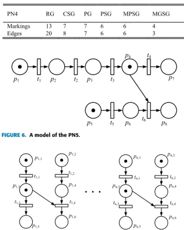
TABLE 1.Algorithms evaluation on PN4.
FIGURE 6. A model of the PN5.
FIGURE 7. Parallel composition of n instances of PN4 (||nPN4).
in Fig. 4(b), (c) and (d), respectively. The evaluation of dif-ferent algorithms on PN4 is summarized in Table 1, focusing on their markings and directed edges labeled by transitions. It is obvious that the size of MGSG is smaller than other state graphs.
The parallel composition of the PN4 is shown in Fig. 7. We exhibit sizes and computing times of various state graphs with respect to these parallel PNs. These state graphs include the reachability graph (RG) computed by the tool TINA, the covering step graph (CSG) proposed in [52], the persistent graph (PG), the persistent step graph (PSG) of [53], the max-imal persistent step graph (MPSG) introduced in [54] and the maximal good step graph (MGSG). The experimental results are shown in Table 2.
Actually, the PSG generalizes PG and any PSG is always smaller than the CSG [53]. For this model, the PSG and the MPSG are identical and the MGSG provides a significant reduction on the number of markings and edges compared with the MPSG.
Then, we consider the model of PN5 shown in Fig. 6. According to Definition 2, there exists a maximal sound stepτ of the initial marking M0= p1+ p4+ p5, i.e.,τ = {t1,
t4, t5}. By Theorem 1, the enabled stepτ is persistent at M0
sinceτ is the only maximal sound step at M0. More precisely,
τ is a maximal good step at M0. Algorithm 1 establishes the
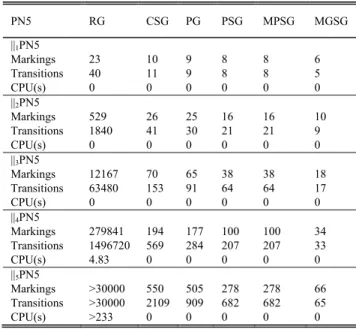
TABLE 2. Experimental results on parallel composition of Fig. 7.
FIGURE 8. The MGSG of the PN5.
For the model of PN5 described in Fig. 6, the evaluation of different algorithms is shown in Table 3. This table summa-rizes the RG, the CSG, the PG, the PSG, the MPSG and the MGSG of PN5, focusing on their numbers of markings and directed edges of transitions, and computing seconds. Fur-thermore, the results of different algorithms on the n parallel PN5 are also shown in Table 3. The parallel composition of n instances of PN5 is represented by ||nPN5.
We can see that the PG is smaller than the CSG, the PSG and the MPSG are identical and the MGSG improves other partial order methods such as the PG, the CSG, and the MPSG.
Next, we consider several PNs of different systems: the FMS (m), the CAS (m), the DP (m), and the SP (m), where m represents the parameter values of their initial markings. The model FMS (m) is a strongly-connected ordinary PN. The model CAS (m) is a strongly-connected loop-free ordi-nary PN, where there exists no transition whose input places are also output places. The dining philosophers is a famous
TABLE 3.Experimental results on parallel composition of the PN5.
model that states an inappropriate use of shared resources generating deadlocks. This DP (m) is a strongly-connected loop-free ordinary PN. The SP (m) is a strongly-connected ordinary PN.
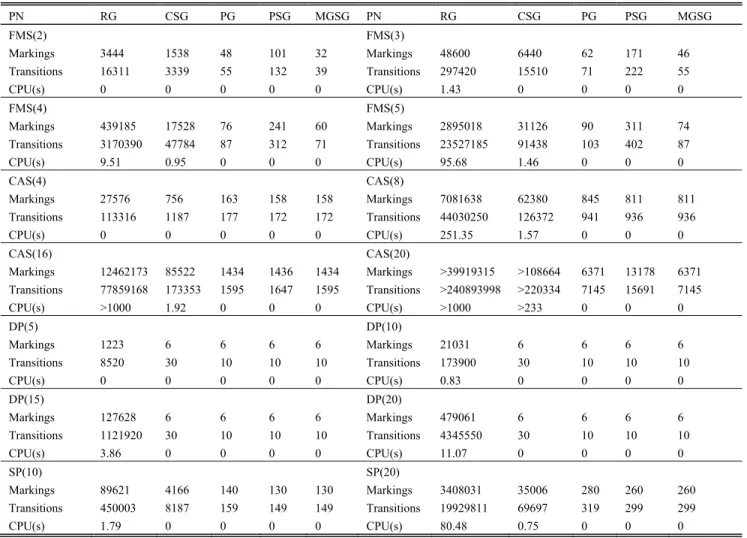
Indeed, MGSG provides a significant reduction on the number of markings and directed edges, and even the com-puting times compared with the RG for each model. In order to illustrate the superiority of the MGSG compared with other reduced graphs obtained by several partial order reduction methods, Table 4 shows the experimental results, including the state graphs computed by TINA such as the RG, the CSG, the PG, and the PSG, and the MGSG established via Algorithm 1. For some PNs such as the FMS (m), the PG provides a smaller graph than CSG and PSG since the firing of steps leads to more intermediate states compared with ones computed after the firing of transitions within persistent sets. Applying the MGSG method, we first obtain the maximal good step, which is a persistent set in essence. Thus, the firing of maximal good steps yields smaller intermediate states than ones obtained by the firing of transitions in persistent sets. It is obvious that the MGSG provides a significant reduction than the PG. For some PNs such as the CAS (m), the parameter of the initial marking influences the size of reduced graphs. Intuitively, the PSG is smaller than the PG when m is less than 8 and the PG is smaller than the PSG when m is higher than 16. For the model of Dining Philosophers, the PG, PSG and the MGSG are identical. The PSG is smaller than the PG and CSG for the model of Swimming Pool. More importantly, the size of CSG, PG, PSG and MGSG does not change, with increasing of parameters of the initial marking. For all these examples, MGSG builds a smaller graph than CSG, PG and PSG. Note that the MGSG technique improves or equals other partial order reduction methods.
TABLE 4. Experimental results on several PNs of different systems.
VI. CONCLUSION AND FUTURE WORK
Although the partial order reduction methods have made some success in alleviating the state space explosion problem of concurrent systems, further improvement is still needed in the state space exploration of large systems. In this paper, we have proposed a new partial order reduction method namely a maximal good step graph (MGSG), based on notions of sound and good steps. Firstly, we present a new definition of sound steps, which breaks the previous require-ment of covering steps. Then, a weaker sufficient condition with practical significance is proposed, to find the set of sound steps at each marking. Next, combining with persis-tent sets and sound steps, the definition of good steps is established and it plays an important role in generating the maximal good step graph (MGSG). The MGSG generation algorithm first determine whether there exists a maximal good step at a marking M . If there exists one, the max-imal good step is fired at M , otherwise the set of maxi-mal sound steps is fired at M . Later, we have proven that the generated maximal good step graph preserves the dead-locks of Petri nets. Finally, the effectiveness of our pro-posed method (MGSG) have been shown via the performed
experimental results. Compared with the covering step graphs, persistent graphs and other reduced reachability graphs combing the above two graphs, the MGSG is more advantageous in state space reduction. In the future, we intend to focus on combining step graphs with any partial order technique as a mean to obtain a more reduction of the state space which is of very great interest for model-checking.
REFERENCES
[1] S. Reveliotis, ‘‘Logical control of complex resource allocation systems,’’ Found. Trends Syst. Control, vol. 4, nos. 1–2, pp. 1–223, 2017. [2] M. Khalgui, O. Mosbahi, and Z. W. Li, ‘‘On reconfiguration theory of
discrete-event systems: From initial specification until final deployment,’’ IEEE Access, vol. 7, pp. 18219–18233, 2019.
[3] K. Barkaoui and H. Boucheneb, ‘‘Introduction to special issue on verifica-tion and evaluaverifica-tion of computer systems,’’ Innov. Syst. Softw. Eng., vol. 14, no. 2, pp. 81–82, 2018.
[4] Y. Qiao, N. Wu, F. Yang, M. Zhou, and Q. Zhu, ‘‘Wafer sojourn time fluctuation analysis of time-constrained dual-arm cluster tools with wafer revisiting and activity time variation,’’ IEEE Trans. Syst., Man, Cybern., Syst., vol. 48, no. 4, pp. 622–636, Apr. 2018.
[5] F. Yang, N. Wu, Y. Qiao, M. Zhou, and Z. Li, ‘‘Scheduling of single-arm cluster tools for an atomic layer deposition process with residency time constraints,’’ IEEE Trans. Syst., Man, Cybern., Syst., vol. 47, no. 3, pp. 502–516, Mar. 2017.
[6] N. Q. Wu and M. C. Zhou, ‘‘Schedulability analysis and optimal scheduling of dual-arm cluster tools with residency time constraint and activity time variation,’’ IEEE Trans. Autom. Sci. Eng., vol. 9, no. 1, pp. 203–209, Jan. 2012.
[7] N. Q. Wu and M. C. Zhou, ‘‘Modeling, analysis and control of dual-arm cluster tools with residency time constraint and activity time vari-ation based on Petri nets,’’ IEEE Trans. Autom. Sci. Eng., vol. 9, no. 2, pp. 446–454, Apr. 2012.
[8] N. Q. Wu, F. Chu, C. B. Chu, and M. C. Zhou, ‘‘Petri net modeling and cycle time analysis of dual-arm cluster tools with wafer revisiting,’’ IEEE Trans. Syst., Man, Cybern., Syst., vol. 43, no. 1, pp. 196–207, Jan. 2013. [9] L. Bai, N. Wu, Z. Li, and M. Zhou, ‘‘Optimal one-wafer cyclic
schedul-ing and buffer space configuration for sschedul-ingle-arm multicluster tools with linear topology,’’ IEEE Trans. Syst., Man, Cybern., Syst., vol. 46, no. 10, pp. 1456–1467, Oct. 2016.
[10] M. Notomi and T. Murata, ‘‘Hierarchical reachability graph of bounded Petri nets for concurrent-software analysis,’’ IEEE Trans. Softw. Eng., vol. 20, no. 5, pp. 325–336, May 1994.
[11] Y. Chen, Z. Li, and K. Barkaoui, ‘‘Maximally permissive liveness-enforcing supervisor with lowest implementation cost for flexible manu-facturing systems,’’ Inf. Sci., vol. 256, no. 1, pp. 74–90, Jan. 2014. [12] Y. Chen, Z. Li, and M. Zhou, ‘‘Behaviorally optimal and structurally simple
liveness-enforcing supervisors of flexible manufacturing systems,’’ IEEE Trans. Syst., Man, Cybern. A, Syst., Humans, vol. 42, no. 3, pp. 615–629, May 2012.
[13] S. Wang, M. Zhou, Z. Li, and C. Wang, ‘‘A new modified reachability tree approach and its applications to unbounded Petri nets,’’ IEEE Trans. Syst., Man, Cybern., Syst., vol. 43, no. 4, pp. 932–940, Jul. 2013.
[14] G. Liu, P. Li, Z. Li, and N. Wu, ‘‘Robust deadlock control for automated manufacturing systems with unreliable resources based on Petri net reach-ability graphs,’’ IEEE Trans. Syst., Man, Cybern., Syst., vol. 49, no. 7, pp. 1371–1385, Jul. 2019. doi:10.1109/TSMC.2018.2815618.
[15] T. Murata, ‘‘Petri nets: Properties, analysis and applications,’’ Proc. IEEE, vol. 77, no. 4, pp. 541–588, Apr. 1989.
[16] J. Ezpeleta, J. M. Colom, and J. Martínez, ‘‘A Petri net based deadlock prevention policy for flexible manufacturing systems,’’ IEEE Trans. Robot. Autom., vol. 11, no. 2, pp. 173–184, Apr. 1995.
[17] X. Guo, S. Wang, D. You, Z. Li, and X. Jiang, ‘‘A siphon-based deadlock prevention strategy for S3PR,’’ IEEE Access, vol. 7, pp. 86863–86873, 2019.
[18] M. Liu, S. Wang, M. Zhou, D. Liu, A. Al-Ahmari, T. Qu, N. Wu, and Z. Li, ‘‘Deadlock and liveness characterization for a class of generalized Petri nets,’’ Inf. Sci., vol. 420, pp. 403–416, Dec. 2017.
[19] D. You, S. Wang, and M. Zhou, ‘‘Computation of strict minimal siphons in a class of Petri nets based on problem decomposition,’’ Inf. Sci., vols. 409–410, pp. 87–100, Oct. 2017.
[20] Q. Zhuang, D. You, W. Dai, S. Wang, and J. Du, ‘‘An iterative deadlock prevention policy based on siphons,’’ in Proc. IEEE 16th Int. Conf. Netw., Sens. Control (ICNSC), Banff, AB, Canada, May 2019, pp. 242–246. [21] C. Zhong, W. He, Z. Li, N. Wu, and T. Qu, ‘‘Deadlock analysis and control
using Petri net decomposition techniques,’’ Inf. Sci., vol. 482, pp. 440–456, May 2019.
[22] K. Barkaoui and I. B. Abdallah, ‘‘A deadlock prevention method for a class of FMS,’’ in Proc. 21st Century IEEE Int. Conf. Syst., Man Cybern. Intell. Syst., Vancouver, BC, Canada, Oct. 1995, pp. 4119–4124.
[23] M. Gan, S. Wang, Z. Ding, M. Zhou, and W. Wu, ‘‘An improved mixed-integer programming method to compute emptiable minimal siphons in S3PR nets,’’ IEEE Trans. Control Syst. Technol., vol. 26, no. 6, pp. 2135–2140, Nov. 2018.
[24] H. Chen, N. Wu, Z. Li, and T. Qu, ‘‘On a maximally permissive deadlock prevention policy for automated manufacturing systems by using resource-oriented Petri nets,’’ ISA Trans., vol. 80, pp. 67–76, Jun. 2019.
[25] Y. Chen, Z. Li, K. Barkaoui, N. Wu, and M. Zhou, ‘‘Compact supervisory control of discrete event systems by Petri nets with data inhibitor arcs,’’ IEEE Trans. Syst., Man, Cybern., Syst., vol. 47, no. 2, pp. 364–379, Feb. 2017.
[26] Y. Chen, Z. Li, A. Al-Ahmari, N. Wu, and T. Qu, ‘‘Deadlock recovery for flexible manufacturing systems modeled with Petri nets,’’ Inf. Sci., vol. 381, pp. 290–303, Mar. 2017.
[27] S. Wang, D. You, and M. Zhou, ‘‘A necessary and sufficient condition for a resource subset to generate a strict minimal siphon in S 4PR,’’ IEEE Trans. Autom. Control, vol. 62, no. 8, pp. 4173–4179, Aug. 2017.
[28] D. You, S. Wang, and C. Seatzu, ‘‘Supervisory control of a class of Petri nets with unobservable and uncontrollable transitions,’’ Inf. Sci., vol. 501, pp. 635–654, Oct. 2019.
[29] N. Ran, S. G. Wang, and W. H. Wu, ‘‘Event feedback supervision for a class of Petri nets with unobservable transitions,’’ IEEE Access, vol. 6, pp. 6920–6926, 2018.
[30] D. You, S. Wang, and W. Hui, ‘‘An algorithm of recognizing unbounded Petri nets with semilinear reachability sets and constructing their reacha-bility trees,’’ IEEE Access, vol. 6, pp. 43732–43742, 2018.
[31] H. Boucheneb, D. Lime, O. H. Roux, and C. Seidner, ‘‘Optimal-cost reachability analysis based on time Petri nets,’’ in Proc. 18th Int. Conf. Appl. Concurrency Syst. Design (ACSD), Jun. 2018, pp. 30–39. [32] Z. Ma, Y. Tong, Z. Li, and A. Giua, ‘‘Basis marking representation of Petri
net reachability spaces and its application to the reachability problem,’’ IEEE Trans. Autom. Control, vol. 62, no. 3, pp. 1078–1093, Mar. 2017. [33] K. Barkaoui and J. F. Pradat-Peyre, ‘‘On liveness and controlled siphons in
Petri nets,’’ in Proc. 17th Int. Conf. Appl. Theory Petri Nets. Osaka, Japan: Springer, 1996, pp.57-72.
[34] C. Chen and H. Hu, ‘‘Liveness-enforcing supervision in AMS-Oriented HAMGs: An approach based on new characterization of siphons using Petri nets,’’ IEEE Trans. Autom. Control, vol. 63, no. 7, pp. 1987–2002, Jul. 2018.
[35] D. You, S. Wang, H. Dou, and W. Duo, ‘‘A resource allocation approach for enforcing liveness on a class of Petri nets,’’ IEEE Access, vol. 6, pp. 48577–48587, 2018.
[36] M. Liu, S. Wang, T. Hayat, A. Alsaedi, and Z. W. Li, ‘‘A resource config-uration method for liveness of a class of Petri nets,’’ IMA J. Math. Control Inf., vol. 33, no. 4, pp. 933–950, Dec. 2016.
[37] K. Barkaoui, J.-M. Couvreur, and K. Klai, ‘‘On the equivalence between liveness and deadlock-freeness in Petri nets,’’ in Proc. Int. Conf. Appl. Theory Petri Nets, Miami, FL, USA, 2005, pp. 90–107.
[38] C. Chen and H. Hu, ‘‘Time-varying automated manufacturing systems and their invariant-based control: A Petri net approach,’’ IEEE Access, vol. 7, pp. 23149–23162, 2019.
[39] P. Godefroid, ‘‘Using partial orders to improve automatic verifica-tion methods,’’ in Proc. 2nd Workshop Comput. Aided Verificaverifica-tion, New Brunswick, NJ, USA, 1990, pp. 176–185.
[40] P. Godefroid, D. Peled, and M. Staskauskas, ‘‘Using partial order methods in the formal validation of industrial concurrent programs,’’ IEEE Trans. Softw. Eng., vol. 22, no. 7, pp. 496–507, Jul. 1996.
[41] P. Godefroid and P. Wolper, ‘‘A Partial approach to model check-ing,’’ in Proc. 6th Annu. IEEE Symp. Logic Comput. Sci., Amsterdam, The Netherlands, Jul. 1991, pp. 406–415.
[42] P. Godefroid and D. Pirottin, ‘‘Refining dependencies improves partial-order verification methods (extended abstract),’’ in Proc. 5th Int. Conf. Comput. Aided Verification, Elounda, Greece, 1993, pp. 438–449. [43] P. Godefroid, J. Van Leeuwen, J. Hartmanis, G. Goos, and P. Wolper,
‘‘Partial-order methods for the verification of concurrent systems: An approach to the state-explosion problem,’’ in Lecture Notes in Computer Science, vol. 1032. Berlin, Germany: Springer, 1996.
[44] R. P. Kurshan, V. Levin, M. Minea, D. Peled, and H. Yenigiin, ‘‘Static partial order reduction,’’ in Proc. Int. Conf. Tools Algorithms Construct. Anal. Syst., 1998, pp. 345–357.
[45] B. Willems and P. Wolper, ‘‘Partial-order methods for model checking: From linear time to branching time,’’ in Proc. 11th Annu. IEEE Symp. Logic Comput. Sci., New Brunswick, NJ, USA, Jul. 1996, pp. 294–303. [46] A. Valmari and H. Hansen, ‘‘Can stubborn sets be optimal?’’ Fundamenta
Informaticae, vol. 113, nos. 3–4, pp. 377–397, 2011.
[47] A. Valmari and H. Hansen, ‘‘Stubborn set intuition explained,’’ in Transac-tions on Petri Nets and Other Models of Concurrency XII. Berlin, Germany: Springer, 2017, pp. 140–165.
[48] A. Valmari, ‘‘A stubborn attack on state explosion,’’ Formal Methods Syst. Des., vol. 1, no. 4, pp. 297–322, 1992.
[49] D. Peled, ‘‘All from one, one for all: On model checking using representa-tives,’’ in Proc. 5th Int. Conf. Comput. Aided Verification, Elounda, Greece, Jun. 1993, pp. 409–423.
[50] D. Peled and T. Wilke, ‘‘Stutter-invariant temporal properties are express-ible without the next-time operator,’’ Inf. Process. Lett., vol. 63, no. 5, pp. 243–246, 1997.
[51] H. Boucheneb and K. Barkaoui, ‘‘Delay-dependent partial order reduc-tion technique for real time systems,’’ Real-Time Syst., vol. 54, no. 2, pp. 278–306, 2018.
[52] F. Vernadat, P. Azéma, and F. Michel, ‘‘Covering step graph,’’ in Proc. 17th Int. Conf. Appl. Theory Petri Nets, Osaka, Japan, 1996, pp. 516–535.
[53] P.-O. Ribet, F. Vernadat, and B. Berthomieu, ‘‘On combining the persistent sets method with the covering steps graph method,’’ in Proc. Int. Conf. Formal Techn. Networked Distrib. Syst.Houston, TX, USA: Springer, 2002, pp. 344-359.
[54] K. Barkaoui, H. Boucheneb, and Z. Li, ‘‘Exploiting local persistency for reduced state space generation,’’ in Proc. 12th Int. Conf. Verification Eval. Comput. Commun. Syst., Grenoble, France, 2018, pp. 166–181. [55] K. Barkaoui and H. Boucheneb, ‘‘On persistency in time Petri nets,’’ in
Proc. 16th Int. Conf. Formal Modeling Anal. Timed Syst., Beijing, China, 2018, pp. 108–124.
[56] Y. Tong, Z. Li, C. Seatzu, and A. Giua, ‘‘Verification of state-based opacity using Petri nets,’’ IEEE Trans. Autom. Control, vol. 62, no. 6, pp. 2823–2837, Jun. 2017.
[57] Z. Ma, Z. Li, and A. Giua, ‘‘Marking estimation in a class of time labelled Petri nets,’’ IEEE Trans. Autom. Control, to be published. doi:10.1109/TAC.2019.2907413.
HAO DOU received the B.S. degree from the School of Information and Electronic Engineering, Zhejiang Gongshang University, China, in 2017, where she is currently pursuing the M.S. degree. Her current research interests include supervisory control of discrete event systems, and Petri nets theory and application.
KAMEL BARKAOUI received the Ph.D. degree and the Habilitation à Diriger des Recherches in computer science from Université Paris 6, in 1988 and 1998, respectively. He is currently a Professor of computer science with the Con-servatoire National des Arts et Métiers, Paris. He has published more than 100 refereed inter-national journal articles and conference papers. His research interests include formal methods for verification, control, and performance evaluation of concurrent and distributed systems. He received the IEEE International Conference on System, Man, and Cybernetics Outstanding Paper Award, in 1995. He has served as the program committee chair and organizing chairs for numerous international workshops and conferences. He was a Guest Editor of the Journal of Systems and Software and the International Journal of Critical Computer-Based Systems.
HANIFA BOUCHENEB is currently a Professor with the École Polytechnique de Montréal. Her research interests include formal verification tech-niques of real-time and infinite complex systems. She has published more than 100 research articles in international journals, conferences, workshops, and books. She has served as a member and as a chair in several program committees of confer-ences and workshops.
XIAONING JIANG received the M.E. degree in electronic engineering from Hangzhou Dianzi University, Hangzhou, China, in 1993, and the Ph.D. degree in computer science and technol-ogy from Zhejiang University, Hangzhou, China, in 2000. He is currently an Associate Professor, a Senior Engineer with Zhejiang Gongshang Uni-versity, and the Vice Dean of the IoT Research Institute, Zhejiang Gongshang University. His research interests include applied information sys-tem, network and information security, industrial IoT, visual analytic, and Fin-tech. He has published over 30 research articles and 10 invention patents.
SHOUGUANG WANG (M’10–SM’12) received the B.S. degree in computer science from the Changsha University of Science and Technology, Changsha, China, in 2000, and the Ph.D. degree in electrical engineering from Zhejiang University, Hangzhou, China, in 2005.
He joined Zhejiang Gongshang University, in 2005, where he is currently a Professor with the School of Information and Electronic Engineer-ing, the Director of the Discrete-Event Systems Group, and the Dean of the System Modeling and Control Research Insti-tute, Zhejiang Gongshang University. He was a Visiting Professor with the Department of Electrical and Computer Engineering, New Jersey Institute of Technology, Newark, NJ, USA, from 2011 to 2012. He was the Dean of the Department of Measuring and Control Technology and Instrument, from 2011 to 2014. He is currently a Visiting Professor with the Electrical and Electronic Engineering Department, University of Cagliari, Cagliari, Italy, from 2014 to 2015. He is also an Associate Editor of IEEE ACCESSand the IEEE/CAA JOURNAL OFAUTOMATICASINICA.