Journal of Geophysical Research: Solid Earth
Variability and origin of seismic anisotropy across
eastern Canada: Evidence from shear wave
splitting measurements
F. A. Darbyshire1, I. D. Bastow2, A. M. Forte1, T. E. Hobbs3, A. Calvel1, A. Gonzalez-Monteza1, and B. Schow4
1Centre de recherche GEOTOP, Université du Québec à Montréal, Montréal, Québec, Canada,2Department of Earth
Science and Engineering, Imperial College London, London, UK,3School of Earth and Atmospheric Sciences, Georgia
Institute of Technology, Atlanta, Georgia, USA,4School of Earth Sciences, Stanford University, Stanford, California, USA
Abstract
Measurements of seismic anisotropy in continental regions are frequently interpreted with respect to past tectonic processes, preserved in the lithosphere as “fossil” fabrics. Models of the present-day sublithospheric flow (often using absolute plate motion as a proxy) are also used to explain the observations. Discriminating between these different sources of seismic anisotropy is particularlychallenging beneath shields, whose thick (≥200 km) lithospheric roots may record a protracted history of deformation and strongly influence underlying mantle flow. Eastern Canada, where the geological record spans ∼3 Ga of Earth history, is an ideal region to address this issue. We use shear wave splitting measurements of core phases such as SKS to define upper mantle anisotropy using the orientation of the fast-polarization direction𝜙 and delay time 𝛿t between fast and slow shear wave arrivals. Comparison with structural trends in surface geology and aeromagnetic data helps to determine the contribution of fossil lithospheric fabrics to the anisotropy. We also assess the influence of sublithospheric mantle flow via flow directions derived from global geodynamic models. Fast-polarization orientations are generally ENE-WSW to ESE-WNW across the region, but significant lateral variability in splitting parameters on a≤100 km scale implies a lithospheric contribution to the results. Correlations with structural geologic and magnetic trends are not ubiquitous, however, nor are correlations with geodynamically predicted mantle flow directions. We therefore consider that the splitting parameters likely record a combination of the present-day mantle flow and older lithospheric fabrics. Consideration of both sources of anisotropy is critical in shield regions when interpreting splitting observations.
1. Introduction
Seismic anisotropy beneath the continents, in particular the ancient continental shields, provides important constraints on past and present tectonic processes, as well as the large-scale patterns of sublithospheric mantle flow. Shear wave splitting analysis is a popular method for studying anisotropy, consisting of point measurements at individual seismograph stations across a region of interest. The resulting splitting parame-ters are interpreted in the context of “fossil” fabrics preserved over long time scales in the lithosphere and/or mineral alignments reflecting mantle flow directions. Beneath the ancient cores of the continents, both factors are likely to play an important role in the depth-averaged anisotropic parameters measured.
When a shear wave encounters such an anisotropic medium, it splits into two orthogonal quasi-shear waves, one traveling faster than the other [e.g., Silver, 1996]. One is orientated along the fast-polarization direction (𝜙) of the anisotropy, and the other is orientated perpendicular. The two waves travel at different speeds; hence, a time lag (𝛿t) is observed between the “fast” and “slow” shear waves when they arrive at the receiver. The size of the lag depends on the thickness of the anisotropic layer and/or the strength of anisotropy. The time lag between the fast and slow components results in nonzero energy on the tangential-component seismogram and an elliptical particle motion. The fast-polarization orientation (𝜙) and time delay (𝛿t) parameters provide simple measurements that characterize seismic anisotropy.
Shear wave splitting parameters can be related to the present-day sublithospheric flow [e.g., Vinnik et al., 1989, 1992; Fouch et al., 2000; Sleep et al., 2002], the preferential orientation of fluid or melt bodies [e.g., Blackman
and Kendall, 1997], preexisting fossil anisotropy frozen in the lithosphere [e.g., Silver and Chan, 1988;
RESEARCH ARTICLE
10.1002/2015JB012228
Key Points:
• SKS splitting measurements show seismic anisotropy variations in eastern Canada
• We investigate the roles of fossil fabrics versus sublithospheric mantle flow
• Both lithospheric and sublithospheric processes contribute to the anisotropy Supporting Information: • Text S1 Correspondence to: F. A. Darbyshire, darbyshire.fi[email protected] Citation:
Darbyshire, F. A., I. D. Bastow, A. M. Forte, T. E. Hobbs, A. Calvel, A. Gonzalez-Monteza, and B. Schow (2015), Variability and origin of seismic anisotropy across eastern Canada: Evidence from shear wave split-ting measurements, J. Geophys.
Res. Solid Earth, 120, 8404–8421,
doi:10.1002/2015JB012228.
Received 20 MAY 2015 Accepted 9 NOV 2015
Accepted article online 17 NOV 2015 Published online 11 DEC 2015
©2015. The Authors.
This is an open access article under the terms of the Creative Commons Attribution-NonCommercial-NoDerivs License, which permits use and distribution in any medium, provided the original work is properly cited, the use is non-commercial and no modifications or adaptations are made.
Vauchez and Nicolas, 1991; Bastow et al., 2007], or combinations of these factors. Seismic phases such as SKS, PKS, and SKKS are ideally suited for shear wave splitting studies of the upper mantle beneath a seismograph station because they involve P-to-S conversions at the core-mantle boundary. No source-side anisotropy is preserved, and these phases are horizontally polarized on exiting the core-mantle boundary [e.g., Savage, 1999]. Near-vertical incidence of the arrivals also results in good lateral resolution.
1.1. Tectonic History
Our study area in eastern Canada samples over 3 Ga of Earth history, from the core of an Archean craton to the coastal edges of a Paleozoic foldbelt (Figure 1). In the northwest, the regional geology is dominated by the Superior craton, the largest Archean craton on Earth. In this part of the Superior, tectonic subprovinces are largely orientated EW and comprise fragments of both continental and oceanic affinity [e.g., Ludden and
Hynes, 2000; Percival, 2007]. The Superior craton is bounded to the east and west by Paleoproterozoic orogenic
belts, the New Quebec Orogen and Trans-Hudson Orogen, respectively [e.g., Hoffman, 1988].
The southeast margin of the craton was affected by several periods of accretion and orogenesis, culminating at ∼1 Ga with the Grenville orogeny, a Himalayan-scale collision associated with the formation of the supercontinent Rodinia [e.g., Whitmeyer and Karlstrom, 2007]. The Grenville province and its boundary with the Superior is complex, with a mix of reworked Archean rocks and younger arc material evident in the surface geology. Crustal-scale seismic studies [e.g., Ludden and Hynes, 2000] suggest that a significant part of the Grenville crust is underlain by Archean material, though the extent of the Archean lithospheric mantle beneath the present-day Grenville belt remains unclear.
The Rodinia supercontinent began to break up in the late Proterozoic. At this time, there is also evidence for a network of failed rift arms in eastern Canada, such as the Ottawa-Bonnechere graben, which developed prior to the opening of the Iapetus ocean [Kamo et al., 1995]. The southeasternmost part of our study region comprises the Appalachian orogenic belts which resulted from the closure of the Iapetus ocean and accretion of numerous continental fragments in the 462–265 Ma time period [e.g., Hatcher, 2005; van Staal, 2005]. The culmination of the collisions marked the assembly of the Pangea supercontinent, which subsequently rifted at ∼180 Ma to form the central North Atlantic ocean.
1.2. Previous Geophysical Studies
Seismic anisotropy beneath eastern North America has been studied through measurements of SKS splitting for over 20 years [e.g., Vinnik et al., 1992; Barruol et al., 1997a; Fouch et al., 2000; Eaton et al., 2004; Frederiksen
et al., 2007]. A lack of seismograph stations throughout much of Quebec and the Atlantic provinces of Canada
has left a large gap in coverage up to recent times; in contrast, the eastern U.S. and much of Ontario have been extensively studied. Across the region, the fast-polarization orientations of SKS splitting are dominated by an ENE-WSW to WNW-ESE trend, as shown from initial sets of measurements at widely spaced seismo-graph stations [e.g., Silver and Chan, 1991; Vinnik et al., 1992; Barruol et al., 1997a]. With the deployment of closely spaced networks and arrays, particularly in eastern Canada, smaller-scale variations became appar-ent. Transects such as Lithoprobe’s Abi-94 and Abi-96 [Sénéchal et al., 1996; Rondenay et al., 2000a] provided a dense coverage of data in a NS line straddling the Grenville Front. Along the transect, the EW average fast orientation of the SKS splits rotated progressively from ENE in the north to ESE in the south. More recently, the deployment of the Portable Observatories for Lithospheric Analysis and Research Investigating Seismic-ity (POLARIS) network [Eaton et al., 2005] afforded a detailed study of anisotropy in southern and eastern Ontario [e.g., Eaton et al., 2004; Frederiksen et al., 2006, 2007]. In this region, complex sublithospheric flow due to a “divot” in the cratonic keel [Fouch et al., 2000] was interpreted to play an important role in variations in
SKSsplitting parameters. Some lithospheric contribution was also inferred, in particular, due to correlation between fast-axis changes over a small length scale with tectonic features such as a failed rift arm [Eaton
et al., 2004; Frederiksen et al., 2006]. Detailed studies made at long-term seismograph stations in New England
[Levin et al., 1999, 2000a, 2000b] showed significant variation of splitting parameters with earthquake back azimuth, leading to the interpretation of two distinct anisotropic layers beneath this region. Bokelmann and
Wüstefeld [2009] compared splitting orientations along the Abi-96 transect to trends in magnetic anomaly
patterns. Though the correlations were variable, particularly around the Grenville Front region, they provided support for a significant contribution to the seismic anisotropy from fossil fabric related to vertically coherent lithospheric deformation from past tectonic events.
In addition to measurements from shear wave splitting alone, seismic anisotropy has been studied beneath continental North America by Yuan and Romanowicz [2010] using a combination of splitting measurements
Journal of Geophysical Research: Solid Earth
10.1002/2015JB012228
Figure 1. (a) Tectonic map of eastern Canada [after Clowes, 2010] and seismograph stations (inverted triangles) used in this study. The pentagon represents six stations of the Charlevoix Array (CA): A11, A16, A21, A54, A64, and LMQ. Regions as follows: ON = Ontario, QC = Québec, NB = New Brunswick, NL = Newfoundland and Labrador, NS = Nova Scotia, ME = Maine (USA). (b) Earthquakes (circles) used inSKSsplitting measurements; the map is centered on our study region (star).
with full-waveform analysis. The results present compelling evidence for significant lithospheric anisotropy across the continent, including multiple layers beneath the stable interior. Similar evidence exists from regional-scale surface wave studies in central and northern Canada [e.g., Darbyshire and Lebedev, 2009;
Darbyshire et al., 2013], as well as global tomographic models [e.g., Debayle and Ricard, 2013].
In this paper, we present new shear wave splitting measurements across eastern Canada from both permanent seismograph stations and more recently installed networks, covering a region that spans Archean, Proterozoic, and Phanerozoic lithosphere. Although station spacing is relatively sparse (∼102 km), these new results
Table 1. List of Seismograph Stations Used in the Studya
Station Code Latitude Longitude Elevation (km) Network Operation A11 47.2425 −70.1978 0.06 CNSN 2000 to the present A16 47.4706 −70.0064 0.02 CNSN 2000 to the present A21 47.7036 −69.6897 0.05 CNSN 2000 to the present A54 47.4567 −70.4125 0.38 CNSN 2000 to the present A64 47.8264 −69.8922 0.14 CNSN 2000 to the present ALFO 45.6283 −74.8842 0.00 POLARIS 2004 to the present BATG 47.2767 −66.0599 0.34 POLARIS 2005 to the present BELQ 47.3980 −78.6874 0.36 POLARIS 2007 to the present CHGQ 49.9105 −74.3748 0.41 POLARIS 2007 to the present DMCQ 48.9646 −72.0680 0.20 POLARIS 2009 to the present GAC 45.7033 −75.4783 0.06 CNSN 1992 to the present GBN 45.4067 −61.5133 0.04 CNSN 2005 to the present GGN 45.1184 −66.8420 0.03 CNSN 2002 to the present ICQ 49.5217 −67.2719 0.06 CNSN 2001 to the present LATQ 47.3836 −72.7819 0.16 POLARIS 2007 to the present LMN 45.8520 −64.8060 0.36 CNSN 1993 to the present LMQ 47.5485 −70.3258 0.43 CNSN 1998 to the present LSQQ 49.0580 −76.9796 0.31 POLARIS 2009 to the present MATQ 49.7589 −77.6376 0.28 POLARIS 2007 to the present NEMQ 51.6837 −76.2576 0.20 POLARIS 2007–2009 NMSQ 51.7133 −76.0237 0.28 POLARIS 2009 to the present SCHQ 54.8324 −66.8332 0.50 CNSN 1998 to the present WEMQ 53.0535 −77.9737 0.17 POLARIS 2005 to the present YOSQ 52.8666 −72.1998 0.65 POLARIS 2005 to the present
aNetwork affiliations are as follows = CNSN: Canadian National Seismograph Network, POLARIS: Portable
Observato-ries for Lithospheric Analysis and Research Investigating Seismicity.
that has until now only been studied in the context of global-/continental-scale tomographic models. The fast-polarization orientations of the seismic anisotropy are initially compared to lithospheric fabrics inferred from surface geological boundaries and potential field data. In order to investigate the potential contribution to the splitting from the present-day mantle flow, we study the horizontal flow directions inferred from a set of global geodynamic models and compare these to the seismic anisotropy data set for eastern Canada.
2. Data Set and Shear Wave Splitting Measurements
Data from 24 broadband seismograph stations in eastern Canada were used in this study. These consist of a group of 12 permanent stations from the Canadian National Seismograph Network (CNSN) and 12 temporary stations installed during the period 2004–2009 and still in operation at present (Table 1). The tem-porary stations were deployed through the POLARIS (Portable Observatories for Lithospheric Analysis and Research Investigating Seismicity) project [Eaton et al., 2005] and related initiatives. All stations transmit data continuously, in real time, to the Canadian National Data Centre. Eight stations lie within the Archean Superior craton, eight are situated within the Proterozoic Grenville Province, and the rest are located on Appalachian terranes in Maritime Canada (Figure 1).
We selected earthquakes of magnitude≥6.0 from the global catalogs, with epicentral distances of 88∘ or more from the center of the network. This distance criterion is necessary to separate core S phases (SKS and SKKS) from nonradially polarized phases such as S and ScS. Following basic data processing, we filtered the seis-mograms between 0.04 and 0.3 Hz, using a two-pole, Butterworth band-pass filter. Where the signal-to-noise ratio was sufficiently high, we analyzed core phases SKS, SKKS, and/or PKS arrivals (hereafter all termed “SKS”).
Journal of Geophysical Research: Solid Earth
10.1002/2015JB012228
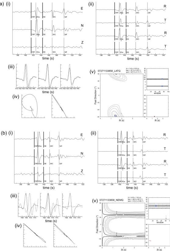
Figure 2. Examples of shear wave splitting analysis. (a) A high-quality split. (i) Original three-component seismogram (east, north, and vertical) showing theSKSphase and subsequent arrivals, along with the chosen analysis window (marked START and END), (ii) radial and tangential components before (top) and after (bottom) correction by the splitting analysis; tangentialSKSenergy is minimized, (iii) windowed waveforms (dashed line: fast, solid line: slow) before and after correction; plot 2 is normalized and plot 3 shows the corrected waves with their relative amplitudes preserved, (iv) particle motion before and after correction, showing the change from elliptical to linearized motion, and (v) grid search and cluster analysis outputs. The main graphic shows the final grid search results for𝜙and𝛿t; the two smaller plots show individual measurements of𝜙and𝛿tfor the 100 windows used in the analysis.
(b) A high-quality null. In this case, there is no signal on the tangential-component waveform, and the particle motion is linear both before and after analysis.
Figure 3. (a) Compilation of individual high-quality splitting measurements for the eastern Canadian stations. Blue bars show splits, and black crosses indicate nulls (showing the 90∘ambiguity). (b) Results of stacking the individual measurements at each station. Ticked lines AF and GF show the Appalachian and Grenville fronts, respectively. CA: Charlevoix array (stations A11, A16, A21, A54, A64, and LMQ).
SKSsplitting measurements were made using the method of Teanby et al. [2004], which is based on the approach of Silver and Chan [1991]. The horizontal-component seismograms are rotated, and one component is time shifted so as to minimize the second eigenvalue of particle motion in the analysis window, lineariz-ing particle motion. A grid search over plausible values of𝜙 and 𝛿t is performed to find the best solution. In the method of Teanby et al. [2004], individual measurements are made over a set of 100 windows around the
SKSarrival, and a cluster analysis is performed to find the most stable splitting parameters𝜙 and 𝛿t, as well as an error analysis and a measurement of the source polarization. Our analysis systematically checks for cor-respondence between event back azimuth and source polarization, to avoid spurious results that would be associated with deep-mantle anomalies, such as those related to the postperovskite phase transition at D’’ [e.g., Restivo and Helffrich, 2006].
SKSsplitting results typically fall into two categories. A split wave initially shows energy on the tangential com-ponent and an elliptical particle motion. When the seismograms are corrected for the optimum𝜙 and 𝛿t, the waveforms will match, the tangential component energy is minimized, and the particle motion is linearized. An example is given in Figure 2a. If the wave passes through azimuthally isotropic material, or if its azimuth is orientated parallel or perpendicular to the fast axis of anisotropy, or if multiple layers of anisotropy cancel out, a characteristic “null” result will be observed (e.g., Figure 2b) [e.g., Barruol and Hoffmann, 1999]. In this case, there will be no energy on the tangential component prior to correction, and the uncorrected particle motion will be linear.
A single, horizontal, homogeneous layer of anisotropy can be characterized by a single pair of splitting param-eters. Systematic variations with earthquake back azimuth may indicate a more complex structure, such as the presence of two or more anisotropic layers [e.g., Levin et al., 1999]. Individual results were thus plotted against the source polarization of the incoming phase (which should be approximately the same as the geometrical back azimuth) to check for complex structure. Where there was no compelling evidence for systematic variation, we used an analysis based on the method of Restivo and Helffrich [1999] to stack the splitting results for each station. The stacks are weighted by signal-to-noise ratio.
3. Results
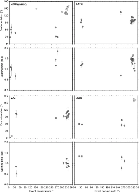
Individual measurements of splitting orientations (Figure 3a) generally cluster relatively tightly around a dom-inant direction, and nulls mostly fall along or perpendicular to this direction. We examined the back azimuthal coverage of the good-quality splitting measurements to ascertain whether there was sufficient evidence of systematic variation in (𝜙, 𝛿t) parameters to infer the presence of multiple anisotropic layers. In the case of our data set, despite long recording times at many of the stations, the measurements are largely confined to one or two relatively restricted back azimuthal ranges (Figure 4). The large gaps in azimuthal coverage do not allow for a direct interpretation of multilayered anisotropic characteristics; therefore, we restrict our
Journal of Geophysical Research: Solid Earth
10.1002/2015JB012228
Figure 4. Examples of the back azimuthal coverage of good-quality splitting results for four representative stations: NEMQ/NMSQ (Superior), LATQ and A54 (Grenville), and GGN (Appalachians). Similar coverage is seen for the rest of the network. For each station, the top graph shows fast orientations; squares represent null measurements, and circles with error bars are splits. The bottom graph shows delay times for the splits only (since𝛿tis undefined for nulls).
Table 2. StackedSKSSplitting Parameters for Each Stationa
Station Code Orientation (∘) Delay Time (s) Number Previous Measurements A11 90±1.25 0.90±0.03 16 A16 −88±1.75 0.83±0.06 9 A21 −87±3.00 0.33±0.02 13 A54 −83±1.25 0.80±0.03 14 A64 −89±1.25 0.63±0.02 22 ALFO 75±2.50 0.88±0.07 4 BATG −86±5.00 0.53±0.03 6 BELQ −83±1.00 0.65±0.02 11 CHGQ −64±2.75 0.70±0.01 7 DMCQ 82±6.25 0.60±0.04 3 GAC 75±2.25 0.48±0.03 12 85∘/0.9 s ; 36∘/0.65 s ; 61±13∘/0.5±0.3 s GBN −84±1.50 0.68±0.03 7 GGN 67±1.00 1.03±0.03 9 ICQ 82±4.75 0.68±0.06 5 LATQ −82±1.00 1.40±0.02 20 LMN 76±1.75 1.15±0.06 5 78∘/1.3 s ; 83∘/1.48 s LMQ 83±2.00 1.03±0.07 7 87∘/1.3 s ; 83∘/1.1 s LSQQ 85±2.00 0.73±0.11 3 MATQ 79±1.00 0.83±0.03 10 NEMQ 43±1.75 0.63±0.10 4 NMSQ 50±1.00 0.63±0.10 17 SCHQ 80±1.00 0.65±0.03 11 WEMQ 62±7.25 0.13±0.02 18 65±52∘/0.75±0.65 s YOSQ 64±1.75 1.33±0.06 6
aNote that the large errors and small delay time value at station WEMQ are due to the abundance of null results at
this station. Results from the literature, where available, are given in pairs of splitting orientation/delay time. Semicolons separate the results of multiple studies or a single study using multiple methods.
quantitative analyses to comparisons with the dominant anisotropic directions inferred from the full sets of measurements. A notable exception is station WEMQ in the north of the study region. The back azimuthal coverage here is slightly better than average, but almost all measurements gave null results.
Given the general consistency in the individual measurements, we stacked the entire ensemble of results for each station; the resulting splitting orientations are shown in Figure 3b and Table 2. The dominant splitting orientations range from NE-SW to NW-SE within a broadly E-W average. We note significant changes in split-ting orientation between individual stations spaced ∼200–300 km apart. Delay times are also highly variable, ranging from ∼0.3 s (A21) to ∼1.4 s (LATQ and YOSQ). The stacks also show a null result for WEMQ. There does not appear to be a systematic large-scale correlation between delay time or splitting orientation and tectonic province; splitting parameters are particularly variable between stations in the Superior craton. Similarly, the behavior of splitting parameters at stations close to major tectonic boundaries does not show a systematic pattern. At BELQ, the splitting orientation lies at a shallow angle to the strike of the Grenville Front; however, CHGQ and SCHQ show boundary-perpendicular angles with respect to the Grenville Front and the New Quebec Orogen boundaries, respectively. The dominant splitting at ICQ is subparallel to the Appalachian Front, whereas the Charlevoix array stations show an E-W fast orientation, ∼30∘ away from the local strike of the Appalachian Front.
4. Discussion
Seismic anisotropy in the upper mantle is most commonly attributed to large-scale structural alignments or mineral orientations arising from past or present strain and deformation. Olivine, the most abundant mineral in the upper mantle, is highly intrinsically anisotropic. Strain arising from mantle flow can result in the
Journal of Geophysical Research: Solid Earth
10.1002/2015JB012228
Figure 5. Comparison of the new stackedSKSsplits (red bars) with previous measurements (purple bars) taken from the global shear wave splitting database [Wüstefeld et al., 2009; Trabant et al., 2012], superimposed on tectonic boundaries [after Clowes, 2010]. The two arrows show absolute plate motion (APM) in two different reference frames: Nuvel-NNR (DeMets et al. [1990]; green) and HS3 (Gripp and Gordon [2002]; black). Ticked lines AF and GF show the Appalachian and Grenville fronts, respectively.
alignment of olivine a axes in the flow direction [e.g., Zhang and Karato, 1995; Bystricky et al., 2000;
Tommasi et al., 2000], resulting in an anisotropic fabric due to the crystallographic-preferred orientation of
olivine, assuming a one-dimensional steady state shear flow [e.g., Kaminski and Ribe, 2002]. Laboratory anal-yses and sampling of mantle xenoliths suggest that the lithospheric mantle is dominated by a-type olivine fabric [Karato et al., 2008]. Evidence exists for other fabric types in the asthenosphere and deep upper mantle; however, away from tectonically active areas such as subduction zones, the anisotropic fabrics likely present would have a similar effect on SKS waves as the a type [Karato et al., 2008].
4.1. Comparison With Previous Studies
Figure 5 shows the stacked splitting results from this study superimposed on those from previous SKS split-ting analyses carried out across the region. The splitsplit-ting parameters are taken from the global SKS splitsplit-ting database compiled by Geosciences Montpellier [Wüstefeld et al., 2009] and mirrored by IRIS [Trabant et al., 2012]. The majority of the new values presented in this study cover regions not previously measured. In areas where our new results overlap with previous studies, the agreement between splitting measurements is largely very good (e.g., stations BELQ and MATQ). Station WEMQ in the NW of the study area (∼53∘N,78∘W) is an obvious exception, exhibiting an extremely small stacked split, since almost all individual measurements at this station were nulls. A previous study using a much smaller data set [Frederiksen et al., 2007] suggested a
larger split; however, the large error bars reported for the splitting parameters suggest that a number of null measurements may have been present.
The vast majority of the seismic anisotropy inferred from shear wave splitting studies is generally attributed to the upper mantle. Lower mantle anisotropy may give rise to source polarization anomalies [e.g., Restivo
and Helffrich, 2006] or to discrepancies in splitting parameters between SKS and SKKS waveforms. These two
phases have similar paths in the upper mantle but can differ by several hundred kilometers in the lower mantle. Niu and Perez [2004] found SKS/SKKS discrepancies at a number of Canadian seismograph stations to the north and west of our study area; however, station SCHQ in eastern Canada did not exhibit this property. In our data set, there are a few cases of SKS/SKKS discrepancy, but they do not appear systematic across the network or for individual station results. We therefore interpret our results in the context of upper mantle anisotropy only.
4.2. Thickness of Anisotropic Layer(s)
Measurements of SKS splitting have good lateral resolution of seismic anisotropy in the presence of closely spaced seismograph networks but poor depth resolution; interpretations are largely based on the assump-tion that the anisotropy is found in the upper mantle and the crust, but this is generally not directly resolvable. Where station spacing is relatively close (∼100 km), Fresnel zone arguments can be used to infer the likely depth of the anisotropy [e.g., Alsina and Snieder, 1995]. Detailed modeling of the depth ranges of anisotropy can only be carried out where a densely spaced seismograph network records multiple SKS measurements at a good back azimuthal coverage [e.g., Liu and Gao, 2011]. It is, however, possible to estimate the thick-ness of an anisotropic layer based on the splitting time, the average shear wave velocity, and the average percentage anisotropy inferred for the layer. To illustrate the likely layer thicknesses associated with our split-ting measurements, we use an average percentage anisotropy of 4% [Savage, 1999] and shear wave velocities of 4.49–4.65 km/s [Schaeffer and Lebedev, 2014]. The layer thickness is given by L ≃𝛿t < Vs> ∕dVswhere < Vs> is the shear wave velocity and dVsis the percentage anisotropy [e.g., Helffrich, 1995]. Splitting times
are highly variable across our study region, ranging from ∼0.35 s to ∼1.5 s. These values would be consis-tent with anisotropic layer thicknesses from ∼40 km to ∼160 km if a single homogeneous horizontal layer is assumed. Thicker anisotropic layers would be possible if two or more layers of different orientation interact subtractively.
4.3. Lithospheric Versus Sublithospheric Sources
Patterns of seismic anisotropy can develop due to the preferential alignment of minerals in the crust and/or mantle, the preferential alignment of fluid or melt, or some combination thereof [Blackman and Kendall, 1997]. Several tectonic/geodynamic processes could lead to such anisotropy, including (1) asthenospheric flow in the direction of absolute plate motion [e.g., Bokelmann and Silver, 2002; Heintz et al., 2003], (2) mantle flow around deep cratonic keels [e.g., Assumpção et al., 2006], and (3) preexisting fossil anisotropy frozen in the lithosphere [e.g., Silver and Chan, 1991; Plomerová and Babuska, 2010; Bastow et al., 2007]. In the following sections, we discuss the implications of our observations for the lithospheric deformation history of the SE Canada region and for the present-day sublithospheric flow.
4.3.1. Evidence for Complex Anisotropy in North America
Surface wave and full-waveform tomographic studies on a global [e.g., Debayle et al., 2005; Debayle and Ricard, 2013] or regional/continental [e.g., Yuan et al., 2011; Darbyshire et al., 2013] scale have provided compelling evi-dence for stratification of seismic anisotropy beneath the North American continent. The tomographic model of Yuan et al. [2011] suggests that beneath the North American craton, the lithosphere can be divided into two distinct layers, based on fast axes of azimuthal anisotropy. The layering is strongest beneath the Archean cratons (especially the Superior), but layer 2 appears to pinch out to the east, beneath Grenville-aged surface geology. A third, deeper layer was interpreted by Yuan et al. [2011] as sublithospheric anisotropy arising from mantle flow, since they noted a broad-scale correlation with regional absolute plate motion (APM) in the HS3 reference frame [Gripp and Gordon, 2002].
Although the azimuthal coverage of our data set precludes a detailed analysis of possible anisotropic layering, the tomographic models lend significant support to the hypothesis that both lithospheric and sublithospheric anisotropy contribute to the shear wave splitting observed in this study.
4.3.2. Layered Mantle Anisotropy and Apparent SKS Isotropy
We note that the apparent isotropic fabric at station WEMQ, dominated by null measurements, is con-sistent with the existence of two anisotropic layers which, beneath WEMQ, may have canceled out the depth-averaged anisotropy. A similar interpretation was made for a station in southern Australia, where
Journal of Geophysical Research: Solid Earth
10.1002/2015JB012228
Figure 6.SKSsplits (red and purple bars) superimposed on a magnetic anomaly map of Canada (Geological Survey of Canada).
analysis of P-S converted phases led to a model of two orthogonal anisotropic layers [Girardin and Farra, 1998], whereas SKS splitting measurements gave a null result [Barruol and Hoffmann, 1999]. Null measurements in continental lithosphere have been observed in several different regions where the most plausible explana-tion would be an interacexplana-tion between multiple anisotropic layers with different orientaexplana-tions; recent examples include the results of Wagner et al. [2012] in the SE USA and Bastow et al. [2015] in NE Brazil.
4.3.3. Relations Between Splitting Orientations and Surface Tectonics
Within the interior of the Superior craton, there appears to be some correlation between splitting orientations and the strike of individual domains and subprovinces, with splitting directions generally lying subparallel to geologic strikes (Figure 5). This trend breaks down close to the craton boundaries, however. In the west (∼80–78∘) splitting orientations lie at a shallow angle to the Grenville Front, in contrast to the almost 90∘ angle observed at station CHGQ. The latter is similar to the angle between the (E-W) splitting measurement at SCHQ and the (N-S) strike of the boundary between the Superior craton and the Paleoproterozoic New Quebec orogen. Similar types of alignment, along with abrupt changes in splitting orientations, were also reported farther north and west in the Canadian Shield [Bastow et al., 2011; Snyder et al., 2013; Frederiksen et al., 2013], associated with the boundaries between the Superior and Western Churchill cratons which collided during the Paleoproterozoic Trans-Hudson Orogeny.
In the Grenville Province, variations in splitting orientation in previous studies have previously been attributed to lithospheric features, such as the Ottawa-Bonnechere Graben (WNW of stations ALFO and GAC [Eaton et al., 2004; Frederiksen et al., 2006]), or to mantle flow variations [Fouch et al., 2000]. Splitting orientations in the Grenville do not show a large variation over distances of 200–300 km; however, delay times are more variable; over twice as great at LATQ than at DMCQ, for example (Figures 3 and 5). In the latter case, lithospheric anisotropy may have been affected by the development of the Saguenay graben [Kumarapeli, 1985]; DMCQ lies at the northernmost tip of this structure. In Maritime Canada (70–60∘W, 43–49∘N), splitting orientations are largely subparallel to the strike of boundaries within the Appalachian terranes, though those on the south shore of New Brunswick show a stronger correlation with the coast, perhaps associated with rift structures of the adjacent Fundy basin (Figure 5).
A direct comparison between tectonic features and SKS measurements implies an assumption of vertically coherent deformation between the crust and the mantle lithosphere [e.g., Silver and Chan, 1988, 1991]. This may occur whether or not the tectonic boundaries themselves are vertical, since the anisotropy generally records the orientation of the large-scale deformation. Tectonic processes such as continental collision or large-scale terrane accretion likely cause some degree of coherent deformation throughout both the crust and the mantle lithosphere, resulting in a broad region (up to several hundred kilometers) of orogen-parallel anisotropy (e.g., the Trans-Hudson Orogen) [Bastow et al., 2011].
4.3.4. Relations Between Splitting Orientations and Potential Fields
Bokelmann and Wüstefeld [2009] carried out an analysis of correlation between shear wave splitting fast
the crust and mantle lithosphere. We examine the new splitting orientations with respect to Bouguer gravity and magnetic anomaly data (source: Geological Survey of Canada). The Bouguer gravity data show very few significant linear trends (with the exception of the Grenville Front low and some highs in Atlantic Canada), but the lineaments and trends in the magnetic data are much more well defined and thus more informative for comparisons with seismic anisotropy (Figure 6).
Magnetic anomalies are often associated with upper crustal fabric due to considerations of the r−3
intensity-distance relationship and of likely Curie depths within the crust. However, in many stable continental regions, the Curie depth may be as deep as the lower crust and may penetrate into the topmost lithospheric mantle beneath cratons [e.g., Bokelmann and Wüstefeld, 2009, and references therein]. Thus, large-scale coher-ent magnetic lineations likely represcoher-ent structural features penetrating the coher-entire crust, which may in turn be associated with lithospheric-scale boundaries and deformation zones. For example, in the SE USA, Wagner
et al. [2012] studied magnetic features corresponding to major tectonic features and noted correspondence
between SKS splitting orientations and such large-scale lineations.
The characteristics of the magnetic anomalies vary significantly with tectonics (Figure 6). Well-defined lineaments are visible within the Superior craton and the Appalachian terranes. In contrast, aside from the large-scale linear trend at the Grenville Front, the structural fabric within much of the Grenville Province shows localized anomalies rather than linear trends. Similar to the comparison with tectonic boundaries, we note that there is a partial correspondence between splitting orientations and the orientations of magnetic fabric in both the Superior and the Appalachian regions; some splits line up well with magnetic lineaments while others deviate by angles of up to ∼45∘. A similar degree of correspondence was noted by Bokelmann and
Wüstefeld [2009] in their analysis of SKS splits in the Abitibi-Grenville region. Many splitting orientations were
shown to have a close correspondence with the predominant directions of magnetic lineaments (as measured by a statistical analysis of degree of alignment), though the results were somewhat variable in nature, espe-cially around the Grenville Front. Angular differences between magnetic trends and SKS splitting orientations peaked around 0 ± 10∘ but nevertheless showed significant spread, just as we observe in our more qualitative treatment.
The lack of coherent magnetic lineaments in many of the parts of the Grenville Province covered by our split-ting data set likely reflects the complexity of the regional tectonic history. The Grenville crust is a combination of reworked Archean and more juvenile material, and Lithoprobe studies [e.g., Hammer et al., 2010] indicate that much of the Grenville Province is underlain by Archean crust at depth. The extent of Archean versus Proterozoic lithospheric mantle beneath the region is still uncertain. Thus, in this region, crustal magnetic anomalies probably do not reflect large-scale lithospheric fabric, whereas those in both the Superior and the Appalachians likely preserve a clearer record of lithospheric fabric and deformation, with coupling between crust and mantle deformation.
4.3.5. The Role of Sublithospheric Flow
In eastern North America, caution must be used when interpreting anisotropy fast axes in the context of sublithospheric mantle flow using correlation with absolute plate motion (APM). In this region, the “APM” direction changes significantly depending on whether one considers the Pacific hot spot (HS) reference frame [Gripp and Gordon, 2002] or the no-net-rotation (NNR) reference frame [DeMets et al., 1990; Argus et al., 2010], as shown by the arrows in Figure 5. In addition, comparison of global upper mantle anisotropy from surface wave tomography with plate motions suggests that basal drag from plate-asthenosphere interaction is likely weak beneath the slower-moving plates [Debayle and Ricard, 2013]. Plate motion calculations for North Amer-ica give speeds of 16–19 mm/yr in the NNR reference frame and 24–29 mm/yr in the HS reference frame, well below the threshold of 4 cm/yr which Debayle and Ricard [2013] quote as the speed at which seismic anisotropy and plate motion correlate well at a full-plate scale.
A more instructive comparison can be made by considering horizontal directions of sublithospheric flow derived from global geodynamic models [e.g., Forte, 2000; Gaboret et al., 2003; Becker et al., 2003]. Accord-ing to the global study of Conrad et al. [2007], simple shear in the asthenosphere rotates the olivine LPO toward the infinite strain axis except for regions close to plate boundaries. Beneath the slow-moving plates, this shear accommodates motion between the relatively stationary lithosphere and the underlying mantle flow, rather than being strongly associated with plate-driven basal drag. These studies of mantle flow-induced deformation have long suggested that asthenospheric anisotropy contributes to SKS splitting measurements for both continental and oceanic regions worldwide. However, while it is a dominant factor for oceanic measurements, deviations between mantle flow and seismic anisotropy measurements for continental
Journal of Geophysical Research: Solid Earth
10.1002/2015JB012228
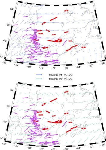
Figure 7. Comparisons betweenSKSsplitting fast orientations and flow-related fabrics from two geodynamic models. Red/purple bars: anisotropy measurements fromSKSsplitting; blue and green arrows: horizontal component of instantaneous mantle flow. The same seismic tomography model but different radial viscosity models are used to calculate the flow magnitudes and directions.
regions again suggest a significant contribution from fossil lithospheric anisotropy. Nevertheless, the relative roles of lithospheric and sublithospheric processes have been debated; some authors [e.g.., Silver and Chan, 1991; Silver and Kaneshima, 1993; Barruol et al., 1997b] suggest that fossil anisotropy dominates beneath Precambrian regions, whereas others [e.g., Vinnik et al., 1992, 1995] consider sublithospheric flow to be the major factor in seismic anisotropy beneath cratons.
In Figure 7 we compare the splitting orientations with mantle flow predictions [Forte et al., 2015] based on the seismic-geodynamic global tomography model TX2008 [Simmons et al., 2009], using two different radial viscosity profiles, “V1” [Mitrovica and Forte, 2004] and “V2” [Forte et al., 2010b]. The main difference between the two profiles in the upper mantle is the thickness of the high-viscosity lithospheric layer: ∼100 km for V1 and ∼200 km for V2. In the following, we consider V1 as having “normal” lithospheric thickness, in the sense of being representative of a globally averaged thickness, whereas V2 has a “thick” lithosphere that may be more representative of subcratonic mantle. The flow calculations are carried out globally up to maximum harmonic degree 128 but are presented here on a finer length scale of 2∘ × 2∘ for comparison with the splitting measurements. Inferred flow directions vary depending on the viscosity profile used in the calculations and are smoothly varying but nonuniform across the region of interest, reflecting the complexities of the mantle buoyancy distribution beneath this region and the role of vertical flow (upwellings and downwellings). In some regions, the spatial scale of variation is similar to that of the splitting parameters, except for regions of dense seismic data coverage. However, the degree of fit between the splitting orientations and modeled flow directions varies from subparallel to subperpendicular (Figure 7); neither of the two flow predictions provides a uniformly good match to the entire range of variability in the splitting orientations.
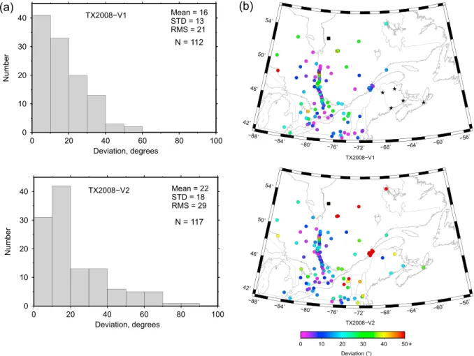
Figure 8. (a) Histogram of angular deviation between shear wave splitting orientations and horizontal mantle flow directions (after correction for the 180∘ ambiguity inherent in the orientations), for mantle flow models TX2008-V1 and TX2008-V2 [Simmons et al., 2009; Mitrovica and Forte, 2004; Forte et al., 2010a]. (b) Maps of angular deviations across eastern Canada for the two different flow models. The black stars in map TX2008-V1 indicate a region where the flow is dominantly radial, precluding a direct comparison withSKSazimuthal anisotropy. The five stations are therefore not included in the V1 histogram in Figure 8a. Station WEMQ (null split) is shown as a black square in the maps.
Although no single radial profile of mantle viscosity (V1 or V2) appears to explain all the splitting measure-ments across the entire geographic span of the study region, it is important to note that each profile does yield matches to the splitting observations in different subregions. The level of fit is quantified in Figure 8b, through maps of angular deviation between flow direction and splitting orientation. We note that in western-most Quebec the V2 (“thicker” lithosphere) predictions provide a better overall fit. In contrast, in south-central Quebec the V1 (“normal” lithosphere) predictions generally provide a better match. It is also notable that under the NE U.S., where seismic tomographic interpretations suggest a lithospheric divot due to the passage of the Great Meteor hot spot [e.g., Eaton and Frederiksen, 2007], the V1 viscosity predictions yield a distinctly better fit to the splitting observations compared to the V2 results (Figures 7 and 8). These correlations reinforce previous studies suggesting that shear wave splitting observations provide potentially important constraints on the effects of lateral variations in lithospheric thickness [e.g., Fouch et al., 2000; Eaton et al., 2004]. This vari-able thickness, equivalent to lateral variations in viscosity, can be modeled in more complex flow simulations that include 3-D viscosity heterogeneity [e.g., Moucha et al., 2007]. Such simulations [e.g., Forte et al., 2010a] may potentially reconcile the splitting measurements with a single mantle flow model. The verification of this hypothesis requires further modeling of the origin and mapping of lateral viscosity variations [e.g., Glišovi´c
et al., 2015] and will be the focus of future work.
In Figure 8a we provide a quantitative summary of the angular deviations calculated between the shear wave splits and the corresponding flow direction. Although the majority of deviations are less than 20∘, several show larger deviations, including near-perpendicular orientations locally. We find that some of the largest deviations occur in regions where the predicted radial flow dominates over the horizontal flow (e.g., for the
Journal of Geophysical Research: Solid Earth
10.1002/2015JB012228
V1 viscosity predictions beneath Maritime Canada in model TX2008-V1; see Figure 7). As discussed above, others occur in regions of substantial horizontal flow such that misfits observed with one viscosity profile (e.g., V1 predictions in central Quebec) are improved using the other. The calculations of deviation also highlight the large variability in splitting orientations over small length scales, such as the dense set of measurements along the Abi-96 transect. This variability is also evident in the individual splitting measurements (Figure 3a). In addition to degrees of match between modeled flow directions and shear wave splitting measurements, Fresnel zone arguments suggest that a significant proportion of the anisotropy likely lies in the upper part of the upper mantle [e.g., Alsina and Snieder, 1995]. Beneath the Archean and Proterozoic domains, the litho-spheric keel is thick:>150 km; closer to ∼200–250 km in many areas [e.g., Schaeffer and Lebedev, 2014], and it is reasonable to expect that “frozen” anisotropic fabric exists within the keel, given the complex tectonic history of the region. Nevertheless, the degree of correlation between the mantle flow models and the split-ting orientations suggests that sublithospheric flow may play an important role in the present-day regional seismic anisotropy patterns.
5. Conclusions
SKS-splitting measurements were performed at 24 broadband seismograph stations in eastern Canada, cov-ering a region that spans approximately three fourths of Earth’s geological history from the Archean to the Phanerozoic. Station-averaged splitting orientations show a broadly E-W pattern across the region as a whole; however, variations in both orientation and delay times are significant at lateral scales of ∼100 km. The split-ting orientations align approximately with surface tectonic features in some regions but make a high angle with both geologic boundaries and magnetic anomaly lineaments in others. Similarly, there is no consis-tent coherence between the splitting orientations and either North American APM or directions of horizontal sublithospheric flow.
The scale of lateral variability suggests that at least part of the anisotropy giving rise to the shear wave splits must originate in the lithosphere, through frozen structural or mineralogical alignments. However, we infer that sublithospheric flow also plays a significant role. We note that the present-day plate motion beneath eastern North America is slow; thus, detailed models of mantle flow rather than a simple treatment related to basal drag of the plate are necessary when considering the sources of sublithospheric anisotropy. The relative roles of fossil lithospheric fabric and sublithospheric flow must be considered carefully in this context. Particular caution is necessary in studies where back azimuthal coverage is limited, leading generally to hypotheses of a single, horizontal, homogeneous layer of anisotropy to explain the shear wave splitting mea-surements. These depth-averaged estimates provide an important first-order constraint on upper mantle anisotropy, but further detailed studies, such as those using surface waves, are necessary to resolve the depths and directions of individual anisotropic layers.
A noteworthy outcome of matching the splitting observations to tomography-based predictions of sublitho-spheric flow is the apparent sensitivity to the thickness of the lithosphere assumed in the flow simulations. This sensitivity shows that shear wave splitting analyses provide important constraints on lateral variations of subcontinental rheology as reflected in the variability of lithospheric thickness.
References
Alsina, D., and R. Snieder (1995), Small-scale sublithospheric continental mantle deformation: Constraints from SKS splitting observations,
Geophys. J. Int., 123, 431–448, doi:10.1111/j.1365-246X.1995.tb06864.x.
Argus, D., R. Gordon, M. Heflin, C. Ma, R. Eanes, P. Willis, W. Peltier, and S. Owen (2010), The angular velocities of the plates and the velocity of Earth’s centre from Space Geodesy, Geophys. J. Int., 180, 913–960, doi:10.1111/j.1365-246X.2009.04463.x.
Assumpção, M., M. Heintz, A. Vauchez, and M. Silva (2006), Upper mantle anisotropy in SE and central Brazil from SKS splitting: Evidence of asthenospheric flow around a cratonic keel, Earth Planet. Sci. Lett., 250(1–2), 224–240, doi:10.1016/j.epsl.2006.07.038.
Barruol, G., and R. Hoffmann (1999), Upper mantle anisotropy beneath the Geoscope stations, J. Geophys. Res., 104, 10,757–10,773, doi:10.1029/1999JB900033.
Barruol, G., P. G. Silver, and A. Vauchez (1997a), Seismic anisotropy in the eastern United States: Deep structure of a complex continental plate, J. Geophys. Res., 102, 8329–8348, doi:10.1029/96JB03800.
Barruol, G., G. Helffrich, and A. Vauchez (1997b), Shear wave splitting around the northern Atlantic: Frozen Pangaean lithospheric anisotropy?, Tectonophysics, 279, 135–148, doi:10.1016/S0040-1951(97)00126-1.
Bastow, I., T. Owens, G. Helffrich, and J. Knapp (2007), Spatial and temporal constraints on sources of seismic anisotropy: Evidence from the Scottish highlands, Geophys. Res. Lett., 34, L05305, doi:10.1029/2006GL028911.
Bastow, I., D. Thompson, J.-M. Kendall, G. Helffrich, J. Wookey, D. Snyder, D. Eaton, and F. Darbyshire (2011), Precambrian plate tectonics: Seismic evidence from Northern Hudson Bay, Geology, 39, 91–94, doi:10.1130/G31396.1.
Acknowledgments
All original seismograms are freely available either through the IRIS Data Management Center or the Canadian National Data Archive via their respective data request tools. A full list of individual splitting measure-ments is provided in the supporting information. Potential field data are available from the Geological Survey of Canada. For mantle flow directions from the global geodynamic models, please contact the authors. Bastow acknowledges support from the Leverhulme Trust (grant P45317). Darbyshire and Forte are funded by NSERC through the Discovery Grants and Canada Research Chairs programs; these programs also funded summer internships for Hobbs, Calvel, and Gonzalez-Monteza. We also acknowl-edge the IRIS Consortium’s summer internship programme (Schow). James Wookey provided the codes and SAC [Goldstein and Snoke, 2005; Helffrich
et al., 2013] macros for the splitting
measurements. Map figures were created using GMT software [Wessel
and Smith, 1998]. We thank the
Editors and two anonymous reviewers for their helpful comments which improved the content of the manuscript.
Bastow, I. D., J. Julià, A. do Nascimento, R. Fuck, T. Buckthorp, and J. McClellan (2015), Upper mantle anisotropy of the Borborema Province, NE Brazil: Implications for intra-plate deformation and sub-cratonic asthenospheric flow, Tectonophysics, 657, 81–93, doi:10.1016/j.tecto.2015.06.024.
Becker, T. W., J. B. Kellogg, G. Ekström, and R. J. O’Connell (2003), Comparison of azimuthal seismic anisotropy from surface waves and finite strain from global mantle-circulation models, Geophys. J. Int., 155, 696–714, doi:10.1046/j.1365-246X.2003.02085.x.
Blackman, D., and J.-M. Kendall (1997), Sensitivity of teleseismic body waves to mineral texture and melt in the mantle beneath a mid-ocean ridge, Philos. Trans. R. Soc. A, 355, 217–231, doi:10.1098/rsta.1997.0007.
Bokelmann, G., and P. Silver (2002), Shear stress at the base of shield lithosphere, Geophys. Res. Lett., 29(23), 2091, doi:10.1029/2002GL015925.
Bokelmann, G. H., and A. Wüstefeld (2009), Comparing crustal and mantle fabric from the North American craton using magnetics and seismic anisotropy, Earth Planet. Sci. Lett., 277, 355–364, doi:10.1016/j.epsl.2008.10.032.
Bystricky, M., K. Kunze, L. Burlini, and J.-P. Burg (2000), High shear strain of olivine aggregates: Rheological and seismic consequences,
Science, 290, 1564–1567, doi:10.1126/science.290.5496.1564.
Clowes, R. (2010), Initiation, development, and benefits of lithoprobe—Shaping the direction of Earth science research in Canada and beyond, Can. J. Earth Sci., 47, 291–314, doi:10.1139/E09-074.
Conrad, C. P., M. D. Behn, and P. G. Silver (2007), Global mantle flow and the development of seismic anisotropy: Differences between the oceanic and continental upper mantle, J. Geophys. Res., 112, B07317, doi:10.1029/2006JB004608.
Darbyshire, F., and S. Lebedev (2009), Rayleigh wave phase-velocity heterogeneity and multilayered azimuthal anisotropy of the Superior Craton, Ontario, Geophys. J. Int., 176, 215–234, doi:10.1111/j.1365-246X.2008.03982.x.
Darbyshire, F. A., D. W. Eaton, and I. D. Bastow (2013), Seismic imaging of the lithosphere beneath Hudson Bay: Episodic growth of the Laurentian mantle keel, Earth Planet. Sci. Lett., 373, 179–193, doi:10.1016/j.epsl.2013.05.002.
Debayle, E., and Y. Ricard (2013), Seismic observations of large-scale deformation at the bottom of fast-moving plates, Earth Planet. Sci. Lett.,
376, 165–177, doi:10.1016/j.epsl.2013.06.02.
Debayle, E., B. Kennett, and K. Priestley (2005), Global azimuthal seismic anisotropy and the unique plate-motion deformation of Australia,
Nature, 433, 509–512, doi:10.1038/nature03247.
DeMets, C., R. Gordon, D. Argus, and S. Stein (1990), Current plate motions, Geophys. J. Int., 101, 425–478, doi:10.1111/j.1365-246X.1990.tb06579.x.
Eaton, D., and A. Frederiksen (2007), Seismic evidence for convection-driven motion of the North American plate, Nature, 446, 428–431, doi:10.1038/nature05675.
Eaton, D., A. Frederiksen, and S.-K. Miong (2004), Shear-wave splitting observations in the lower Great Lakes region: Evidence for regional anisotropic domains and keel-modified asthenospheric flow, Geophys. Res. Lett., 31, L07610, doi:10.1029/2004GL019438.
Eaton, D., et al. (2005), Investigating Canada’s lithosphere and earthquake hazards with portable arrays, Eos Trans. AGU, 86(17), 169–173. Forte, A., R. Moucha, N. Simmons, S. Grand, and J. Mitrovica (2010a), Deep-mantle contributions to the surface dynamics of the North
American continent, Tectonophysics, 481, 3–15, doi:10.1016/j.tecto.2009.06.010.
Forte, A., N. Simmons, and S. Grand (2015), Constraints on seismic models from other disciplines—Constraints on 3-D seismic models from global geodynamic observables: Implications for the global mantle convective flow, in Treatise of Geophysics, 2nd ed., vol. 1, edited by B. Romanowicz and A. Dziewonski, pp. 853–907, Elsevier, Amsterdam, doi:10.1016/B978-0-444-53802-4.00028-2.
Forte, A. M. (2000), Seismic-geodynamic constraints on mantle flow: Implications for layered convection, mantle viscosity, and seismic anisotropy in the deep mantle, in Earth’s Deep Interior: Mineral Physics and Tomography From the Atomic to the Global Scale, Geophys.
Monogr. Ser., vol. 117, edited by A. M. Forte, pp. 3–36, AGU, Washington D. C., doi:10.1029/GM117p0003.
Forte, A. M., S. Quéré, R. Moucha, N. A. Simmons, S. P. Grand, J. X. Mitrovica, and D. B. Rowley (2010b), Joint seismic–geodynamic-mineral physical modelling of African geodynamics: A reconciliation of deep-mantle convection with surface geophysical constraints, Earth
Planet. Sci. Lett., 295, 329–341, doi:10.1016/j.epsl.2010.03.017.
Fouch, M. J., K. M. Fischer, E. Parmentier, M. E. Wysession, and T. J. Clarke (2000), Shear wave splitting, continental keels, and patterns of mantle flow, J. Geophys. Res., 105(B3), 6255–6275, doi:10.1029/1999JB900372.
Frederiksen, A., I. Ferguson, D. Eaton, S.-K. Miong, and E. Gowan (2006), Mantle fabric at multiple scales across an Archean-Proterozoic boundary, Grenville Front, Canada, Phys. Earth Planet. Inter., 158, 240–263, doi:10.1016/j.pepi.2006.03.025.
Frederiksen, A., S.-K. Miong, F. Darbyshire, D. Eaton, S. Rondenay, and S. Sol (2007), Lithospheric variations across the Superior Province, Ontario, Canada: Evidence from tomography and shear wave splitting, J. Geophys. Res., 112, B07318, doi:10.1029/2006JB004861. Frederiksen, A., I. Deniset, O. Ola, and D. Toni (2013), Lithospheric fabric variations in central North America: Influence of rifting and Archean
tectonic styles, Geophys. Res. Lett., 40, 4583–4587, doi:10.1002/grl.50879.
Gaboret, C., A. Forte, and J.-P. Montagner (2003), The unique dynamics of the Pacific Hemisphere mantle and its signature on seismic anisotropy, Earth Planet. Sci. Lett., 208, 219–233, doi:10.1016/S0012-821X(03)00037-2.
Girardin, N., and V. Farra (1998), Azimuthal anisotropy in the upper mantle from observations ofP-to-Sconverted phases: Application to southeast Australia, Geophys. J. Int., 133, 615–629, doi:10.1046/j.1365-246X.1998.00525.x.
Glišovi´c, P., A. M. Forte, and M. W. Ammann (2015), Variations in grain size and viscosity based on vacancy diffusion in minerals, seismic tomography, and geodynamically inferred mantle rheology, Geophys. Res. Lett., 42, 6278–6286, doi:10.1002/2015GL065142. Goldstein, P., and A. Snoke (2005), SAC availability for the IRIS community, DMS Electron. Newsl., 7, 6 pp.
Gripp, A., and R. Gordon (2002), Young tracks of hotspots and current plate velocities, Geophys. J. Int., 150, 321–361, doi:10.1046/j.1365-246X.2002.01627.x.
Hammer, P. T., R. M. Clowes, F. A. Cook, A. J. van der Velden, and K. Vasudevan (2010), The lithoprobe trans-continental lithospheric cross sections: Imaging the internal structure of the North American continent, Can. J. Earth Sci., 47, 821–857, doi:10.1139/E10-036. Hatcher, R. D., Jr. (2005), Southern and central Appalachians, in Encyclopedia of Geology, edited by R. Selley, L. Cocks, and I. Plinner,
pp. 72–81, Elsevier and Academic Press, Amsterdam.
Heintz, M., A. Vauchez, M. Assumpção, G. Barruol, and M. Egydio-Silva (2003), Shear wave splitting in SE Brazil: An effect of active or fossil upper mantle flow, or both?, Earth Planet. Sci. Lett., 211, 79–95, doi:10.1016/S0012-821X(03)00163-8.
Helffrich, G. (1995), Lithospheric deformation inferred from teleseismic shear wave splitting observations in the United Kingdom,
J. Geophys. Res., 100, 18,195–18,204, doi:10.1029/95JB01572.
Helffrich, G., J. Wookey, and I. Bastow (2013), The Seismic Analysis Code: A Primer and User’s Guide, Cambridge Univ. Press, Cambridge, U. K. Hoffman, P. (1988), United plates of America, the birth of a craton: Early Proterozoic assembly and growth of Laurentia, Annu. Rev. Earth
Planet. Sci., 16, 543–603, doi:10.1146/annurev.ea.16.050188.002551.
Kaminski, É., and N. M. Ribe (2002), Timescales for the evolution of seismic anisotropy in mantle flow, Geochem. Geophys. Geosyst., 3(8), 1051, doi:10.1029/2001GC000222.
Journal of Geophysical Research: Solid Earth
10.1002/2015JB012228
Kamo, S., T. Krogh, and P. Kumarapeli (1995), Age of the Grenville dyke swarm, Ontario-Quebec: Implication for the timing of Iapetan rifting,
Can. J. Earth Sci., 32, 273–280, doi:10.1139/e95-022.
Karato, S.-I., H. Jung, I. Katayama, and P. Skemer (2008), Geodynamic significance of seismic anisotropy of the upper mantle: New insights from laboratory studies, Annu. Rev. Earth Planet. Sci., 36, 59–95, doi:10.1146/annurev.earth.36.031207.124120.
Kumarapeli, P. (1985), Vestiges of Iapetan rifting in the craton west of the northern Appalachians, Geosci. Can., 12, 54–59.
Levin, V., W. Menke, and J. Park (1999), Shear wave splitting in the Appalachians and the Urals: A case for multilayered anisotropy, J. Geophys.
Res., 104, 17,975–17,993, doi:10.1029/1999JB900168.
Levin, V., J. Park, M. Brandon, and W. Menke (2000a), Thinning of the upper mantle during late Paleozoic Appalachian orogenesis, Geology,
28, 239–242, doi:10.1130/0091-7613.
Levin, V., W. Menke, and J. Park (2000b), No regional anisotropic domains in the northeastern U.S. Appalachians, J. Geophys. Res., 105(B8), 19,029–19,042, doi:10.1029/2000JB900123.
Liu, K. H., and S. S. Gao (2011), Estimation of the depth of anisotropy using spatial coherency of shear-wave splitting parameters,
Bull. Seismol. Soc. Am., 101, 2153–2161, doi:10.1785/0120100258.
Ludden, J., and A. Hynes (2000), The Lithoprobe Abitibi-Grenville transect: Two billion years of crust formation and recycling in the Precambrian Shield of Canada, Can. J. Earth Sci., 37, 459–476, doi:10.1139/e99-120.
Mitrovica, J., and A. Forte (2004), A new inference of mantle viscosity based upon joint inversion of convection and glacial isostatic adjustment data, Earth Planet. Sci. Lett., 225, 177–189, doi:10.1016/j.epsl.2004.06.005.
Moucha, R., A. Forte, J. Mitrovica, and A. Daradich (2007), Lateral variations in mantle rheology: Implications for convection related surface observables and inferred viscosity models, Geophys. J. Int., 169, 113–135, doi:10.1111/j.1365-246X.2006.03225.x.
Niu, F., and A. M. Perez (2004), Seismic anisotropy in the lower mantle: A comparison of waveform splitting ofSKSandSKKS, Geophys. Res.
Lett., 31, L24612, doi:10.1029/2004GL021196.
Percival, J. (2007), Geology and metallogeny of the Superior Province, Canada, in Mineral Deposits of Canada: A Synthesis of Major
Deposit-Types, District Metallogeny, the Evolution of Geological Provinces and Exploration Methods, Geol. Assoc. Can. Miner. Deposits Div., Spec. Publ., vol. 5, edited by W. Goodfellow, pp. 903–928, Geol. Assoc. of Can. Miner. Deposits Div., Canada.
Plomerová, J., and V. Babuska (2010), Long memory of mantle lithosphere fabric—European LAB constrained from seismic anisotropy,
Lithos, 120, 131–143, doi:10.1016/j.lithos.2010.01.008.
Restivo, A., and G. Helffrich (1999), Teleseismic shear wave splitting measurements in noisy environments, Geophys. J. Int., 137, 821–830, doi:10.1046/j.1365-246x.1999.00845.x.
Restivo, A., and G. Helffrich (2006), Core-mantle boundary structure investigated usingSKSandSKKSpolarization anomalies, Geophys. J.
Int., 165, 288–302, doi:10.1111/j.1365-246X.2006.02901.x.
Rondenay, S., M. Bostock, T. Hearn, D. White, and R. Ellis (2000a), Lithospheric assembly and modification of the SE Canadian Shield: Abitibi-Grenville teleseismic experiment, J. Geophys. Res., 105, 13,735–13,755, doi:10.1029/2000JB900022.
Savage, M. (1999), Seismic anisotropy and mantle deformation: What have we learned from shear wave splitting, Rev. Geophys., 37, 65–106, doi:10.1029/98RG02075.
Schaeffer, A., and S. Lebedev (2014), Imaging the North American continent using waveform inversion of global and USArray data, Earth
Planet. Sci. Lett., 402, 26–41, doi:10.1016/j.epsl.2014.05.014.
Sénéchal, G., S. Rondenay, M. Mareschal, J. Guilbert, and G. Poupinet (1996), Seismic and electrical anisotropies in the lithosphere across the Grenville Front, Canada, Geophys. Res. Lett., 23, 2255–2258, doi:10.1029/96GL01410.
Silver, P. (1996), Seismic anisotropy beneath the continents: Probing the depths of geology, Annu. Rev. Earth Planet. Sci., 24, 385–432, doi:10.1146/annurev.earth.24.1.385.
Silver, P., and W. Chan (1988), Implications for continental structure and evolution from seismic anisotropy, Nature, 335, 34–39, doi:10.1038/335034a0.
Silver, P., and S. Kaneshima (1993), Constraints on mantle anisotropy beneath Precambrian North America from a transportable teleseismic experiment, Geophys. Res. Lett., 20, 1127–1130, doi:10.1029/93GL00775.
Silver, P. G., and W. W. Chan (1991), Shear wave splitting and subcontinental mantle deformation, J. Geophys. Res., 96, 16,429–16,454, doi:10.1029/91JB00899.
Simmons, N. A., A. M. Forte, and S. P. Grand (2009), Joint seismic, geodynamic and mineral physical constraints on three-dimensional mantle heterogeneity: Implications for the relative importance of thermal versus compositional heterogeneity, Geophys. J. Int., 177, 1284–1304, doi:10.1111/j.1365-246X.2009.04133.x.
Sleep, N., C. Ebinger, and J.-M. Kendall (2002), Deflection of mantle plume material by cratonic keels, Geol. Soc. London Spec. Publ., 199, 135–150, doi:10.1144/GSL.SP.2002.199.01.08.
Snyder, D., R. Berman, J.-M. Kendall, and M. Sanborn-Barrie (2013), Seismic anisotropy and mantle structure of the Rae craton, central Canada, from joint interpretation ofSKSsplitting and receiver functions, Precambrian Res., 232, 189–208, doi:10.1016/j.precamres.2012.03.003.
Teanby, N., J.-M. Kendall, and M. Van der Baan (2004), Automation of shear-wave splitting measurements using cluster analysis, Bull. Seismol.
Soc. Am., 94, 453–463, doi:10.1785/0120030123.
Tommasi, A., D. Mainprice, G. Canova, and Y. Chastel (2000), Viscoplastic self-consistent and equilibrium-based modeling of olivine lattice preferred orientations: Implications for the upper mantle seismic anisotropy, J. Geophys. Res., 105, 7893–7908, doi:10.1029/1999JB900411.
Trabant, C., A. R. Hutko, M. Bahavar, R. Karstens, T. Ahern, and R. Aster (2012), Data products at the IRIS DMC: Stepping stones for research and other applications, Seismol. Res. Lett., 83(5), 846–854, doi:10.1785/0220120032.
van Staal, C. (2005), Northern appalachians, in Encyclopedia of Geology, edited by R. Selley, L. Cocks, and I. Plinner, pp. 72–81, Elsevier and Academic Press, Amsterdam.
Vauchez, A., and A. Nicolas (1991), Mountain building: Strike-parallel motion and mantle anisotropy, Tectonophysics, 185, 183–201, doi:10.1016/0040-1951(91)90443-V.
Vinnik, L., V. Farra, and B. Romanowicz (1989), Azimuthal anisotropy in the Earth from observations ofSKSat Geoscope and NARS broadband stations, Bull. Seismol. Soc. Am., 79, 1542–1558.
Vinnik, L., L. Makeyeva, A. Milev, and A. Y. Usenko (1992), Global patterns of azimuthal anisotropy and deformations in the continental mantle, Geophys. J. Int., 111, 433–447, doi:10.1111/j.1365-246X.1992.tb02102.x.
Vinnik, L., R. Green, and L. Nicolaysen (1995), Recent deformations of the deep continental root beneath southern Africa, Nature, 375, 50–52, doi:10.1038/375050a0.
Wagner, L. S., M. D. Long, M. D. Johnston, and M. H. Benoit (2012), Lithospheric and asthenospheric contributions to shear-wave splitting observations in the southeastern United States, Earth Planet. Sci. Lett., 341–344, 128–138, doi:10.1016/j.epsl.2012.06.020.
Wessel, P., and W. Smith (1998), New, improved version of Generic Mapping Tools released, Eos Trans. AGU, 79, 579–579. Whitmeyer, S., and K. Karlstrom (2007), Tectonic model for the proterozoic growth of North America, Geosphere, 3, 220–259,
doi:10.1130/GES00055.1.
Wüstefeld, A., G. Bokelmann, G. Barruol, and J.-P. Montagner (2009), Identifying global seismic anisotropy patterns by correlating shear-wave splitting and surface-wave data, Phys. Earth Planet. Inter., 176(3), 198–212, doi:10.1016/j.pepi.2009.05.006.
Yuan, H., and B. Romanowicz (2010), Lithospheric layering in the North American craton, Nature, 466, 1063–1069, doi:10.1038/nature09332. Yuan, H., B. Romanowicz, K. Fischer, and D. Abt (2011), 3-D shear wave radially and azimuthally anisotropic velocity model of the North
American upper mantle, Geophys. J. Int., 184, 1237–1260, doi:10.1111/j.1365-246X.2010.040901.x.
Zhang, S., and S.-I. Karato (1995), Lattice preferred orientation of olivine aggregates deformed in simple shear, Nature, 375, 774–777, doi:10.1038/375774a0.


![Figure 5. Comparison of the new stacked SKS splits (red bars) with previous measurements (purple bars) taken from the global shear wave splitting database [Wüstefeld et al., 2009; Trabant et al., 2012], superimposed on tectonic boundaries [after Clowes, 20](https://thumb-eu.123doks.com/thumbv2/123doknet/3072485.86772/9.918.100.830.140.704/comparison-previous-measurements-splitting-wüstefeld-superimposed-tectonic-boundaries.webp)