To cite this document:
Smith, Guillaume and Lochin, Emmanuel and Lacan,
Jérôme and Boreli, Roksana Memory and Complexity Analysis of On-the-Fly
Coding Schemes for Multimedia Multicast Communications. (2012) In:
Interntional Conference on Communications (ICC) 2012, 10-15 Jun 2012,
Ottawa, Canada.
O
pen
A
rchive
T
oulouse
A
rchive
O
uverte (
OATAO
)
OATAO is an open access repository that collects the work of Toulouse researchers and
makes it freely available over the web where possible.
This is an author-deposited version published in:
http://oatao.univ-toulouse.fr/
Eprints ID: 5902
Any correspondence concerning this service should be sent to the repository
Memory and Complexity Analysis of On-the-Fly
Coding Schemes for Multimedia Multicast
Communications
Guillaume Smith
Universit´e de Toulouse - ISAE UNSW - NICTA [email protected]
Emmanuel Lochin and
J´erˆome Lacan
Universit´e de Toulouse - ISAE [email protected] and
Roksana Boreli
UNSW - NICTA [email protected]
Abstract—A new class of erasure codes for delay-constraint
applications, called on-the-fly coding, have recently been in-troduced for their improvements in terms of recovery delay and achievable capacity. Despite their promising characteristics, little is known about the complexity of the systematic and non-systematic variants of this code, notably for live multicast transmission of multimedia content which is their ideal use case. Our paper aims to fill this gap and targets specifically the metrics relevant to mobile receivers with limited resources: buffer size requirements and computation complexity of the receiver. As our contribution, we evaluate both code variants on uniform and bursty erasure channels. Results obtained are unequivocal and demonstrate that the systematic codes outperform the non-systematic ones, in terms of both the buffer occupancy and computation overhead.
I. INTRODUCTION
There exist two classes of reliability mechanisms based, re-spectively, on retransmission and redundancy schemes. Auto-matic Repeat reQuest (ARQ) schemes recover all lost packets by utilizing retransmissions. As a consequence, the recovery of a lost packet incurs a delay of at least one additional Round Trip Time (RTT). However, this might not be suitable for time constrained applications, that define a threshold above which they consider a packet outdated and no longer useful to the receiving application. A well-known solution to prevent this additional delay is to add redundancy packets to the data flow. This can be done by using erasure coding schemes. These schemes can be classified into two major groups: block and on-the-fly codes. The main principle of a block code is to usek source packets to sendn encoded packets (with n > k), which are built from the k packets using the encoding mechanism. The addition of n − k repair packets to a block of k source packets allows the decoder on the receiving end to rebuild all of thek source packets if, from the n sent packets, a maximum of n − k packets are lost. If more than (n − k) losses occur within any block, decoding becomes impossible, as the coding mechanism is tightly coupled to a specific block size n.
To overcome this issue, other recent approaches have pro-posed on-the-fly coding schemes [1][2][3], which belongs to a class of convolutional codes. In [1], the authors use
non-binary convolutional codes and show that the decoding delay can be reduced with the use of a sliding window, rather than a block, to generate the repair packets. More recently in [2] and [3], the authors propose an on-the-fly coding scheme that implements an elastic encoding window and uses an unreliable reverse feedback path (when available), to decrease the encoding complexity at the sender side, without impacting the communication data transfer. Compared to [1], both proposals enable a fully reliable service under certain conditions. However, the main difference between [2] and [3] is that the former proposes a non-systematic scheme while the later uses a systematic variant.
In this paper, our aim is to assess the benefit and imple-mentation requirements of both variants of on-the-fly coding schemes, in terms of receiver buffer occupancy and com-putation overhead. The objective is to evaluate the applica-bility of such coding schemes in the context of multimedia communications over multicast services. In particular, the resulting analysis would enable us to determine whether such coding schemes are practical in a multicast environment where the multicast group, comprising of mobile devices (PDAs, cell-phones, etc.) which have lower processing capabilities and limited resources, is receiving, e.g. video or any other multimedia content.
We detail in Section II the characteristics of on-the-fly coding schemes compared to block codes. Then, we analyse the buffer size requirements of such codes over a uniform erasure channel in Section IV while Section V addresses their computation complexity. We also present a study of buffer sizes and computation complexity over a bursty erasure channel in Section VI. Finally we conclude this work in Section VII.
II. BLOCKVERSUSON-THE-FLYCODES
As outlined in the introduction, block codes are defined by two parameters: (k, n) with n > k (from k source data packets,n encoded packets are sent). The difference between various block codes (e.g. LDPC [4] or Reed Solomon codes [5]) is related to the specific linear combination method used
to create repair packets. The difference is reflected in both the encoding/decoding complexity and correction capability. On-the-fly codes are based on the same principle, but also include memory. Therefore, on-the-fly coding schemes are defined by three parameters: (k, n, m) as they are usually based on a sliding encoding window of sizek × m. To encode n packets which will be sent on the network, k × m previous information packets are used [1]. They are referred to as codes with memory as a block of k source packets must be stored to encode them following encoded blocks.
The main feature of these codes is that they are more suitable for bursty erasure channels than the block codes [6], as the information from the source data packets is spread over more than one block (e.g. over m blocks), making the transmission more resistant to bursts of losses.
Neither block nor convolutional codes proposed by [1] use acknowledgements, and as a result, they cannot enable full reliability. One possible solution would be to combine ARQ with such mechanisms. This solution, known as Hybrid ARQ [7], may not be feasible on links which have a long delay, as the missing packets might be retransmitted too late for the multimedia application to use them. To handle this problem, authors in [2] and [3] propose to use an on-the-fly code with an infinite encoding memory (referred to as elastic encoding window) and an acknowledgement path, used to decrease the number of packets in the encoding window. The acknowledge-ment packets are only used, when possible, to decrease the encoding complexity. Obviously, when receivers are mobile devices with limited resources like memory or processing power, an infinite window size is not feasible. We thus propose in this paper to assess the buffer size requirements of the elastic window encoding schemes, including the systematic and non-systematic variants.
To simplify the study, we assume that the on-the-fly code is rateless, similarly to the Fountain codes (e.g. LT [8] or Raptor codes [9]), i.e. the code can create an infinite number of linear combinations (encoded or repair packets) from a finite number of source packets.
We note that the concept of infinite encoding window size has already been used in several contexts. In network coding, this approach enables the creation of ”infinite” linear combinations of packets [10]. In this context, the purpose of having an infinite window is not to protect the data, but to fully use the network capacity, by sending only useful packets to every receiver (a packet is called useful when it is utilised at the receiver side to retrieve missing packets). In this case, only linear combinations of source data packets are sent i.e. the code is non-systematic. In [10], the authors use the concept of a ”seen” packet, which enables the receiver to acknowledge a source data packet Pi when a repair packet, that contains a
linear combination including Pi, is received. More precisely,
Pi is acknowledged by a repair packet whenPiis the first not
yet seen packet contained in this repair packet. This allows the receivers to acknowledge packets (even) before decoding them, thus enabling the source to reduce the size of the encoding window [2]. packet number encoding window non systematic sending systematic sending P1 P1 P1 P1 P2 P1, P2 P 2 1Pi P2 P3 P1, P2, P3 2 ×P 3 1Pi P3 andP 3 1Pi P4 P1to P4 P 4 1Pi P4 P5 P1to P5 P 5 1Pi P5 P6 P1to P6 2 ×P 6 1Pi P6 andP 6 1Pi TABLE I
REPRESENTATION OF THE SOURCE ENCODING WINDOW AND THE SENDING PATTERN IN BOTH SCENARIO FOR A CODE(3, 4). COEFFICIENTS IN THE LINEAR OPERATIONS ARE NOT REPRESENTED,PLEASE NOTE THEY
ARE CHOSEN TO HAVE AMAXIMUMDISTANCESEPARABLE CODE.
In [3], the authors propose to use an on-the-fly code with an infinite encoding window to protect the data. However, the main objective is to enable a fully reliable coding scheme for real-time applications such as VoIP or streaming video. This code is systematic, i.e. the source data are not encoded. Table I illustrates the difference between the on-the-fly coding schemes proposed in [10] and [3].
To the best of our knowledge, there is no existing study that quantifies the complexity and analyses the buffer size requirements of convolutional codes with an infinite encoding window. In a point to point scenario, the analysis is trivial as the systematic codes would logically produce an improvement in terms of delay. However in a multicast context, it is much more complex to estimate the impact of the multicast group size on each receiver within the group. We thus propose to study this problem in the following sections.
III. SIMULATIONSCENARIO ANDPARAMETERS
We have implemented both version (systematic [2] and non-systematic [3]) elastic window codes in Matlab. We use a satellite-like multicast scenario where the source transmits to a number of independent receivers. We vary the number of receivers between 2 to 30. Although the number of receivers in a multicast group consisting of mobile devices may be significantly larger, we will show that the number of receivers used is sufficient to illustrate the differences between the two codes in terms of memory and complexity, as related to the group size.
Matlab is not a real-time simulator, so it was necessary to define a time scale i.e. a unit of time. During this period, the source may receive an ACK (if any), reduce its encoding window, or send a packet; the receivers may receive a packet, decode the repair packets, reduce their buffer sizes, or send an ACK (if needed). TheRT T and the time elapsed between two acknowledgements,s, will consequently be expressed as a multiple of this unit of time.
To simplify the simulation, the matrices used in the encod-ing and decodencod-ing process are not created, therefore avoidencod-ing the need for complex operations like matrix inversion. We also assume that the codes used are maximum distance separable (MDS). As the encoding is based on MDS properties, we only
consider that if a matrix is square, it can be inverted and the decoding is therefore possible.
For our simulations, we always use a code (3, 4) (which can correct up to 25% of erased packets), a packet error rate P ER = 20% and an RT T = 2. For simplicity, we consider an identical delay on the uplink and downlink between the source and the receiver, equal to one unit of time. We vary the number of receivers ands. We evaluate two cases: a uniform erasure channel and a bursty erasure channel. We consider that the links to the different receivers are independent, i.e. the losses (either bursty or uniform, as appropriate to the channel) are independent on both the uplink and the downlink. We note that for all the figures in this paper, each point in any of the graphs represents the average value obtained by 10 simulations, with each simulation consisting of the encoding and decoding process for 10000 data packets.
IV. ANALYSIS OFBUFFERSIZEREQUIREMENTS FOR A
UNIFORMERASURECHANNEL
In this section, we evaluate the buffer size requirements of both systematic and non-systematic codes as a function of s and the number of multicast receivers. Of interest is the required buffer size in the sender and, most importantly (due to resource limitations) the receivers.
The simulation results obtained for both codes over a uniform erasure channel are shown in Fig. 1. We show: the average and the maximum number of packets in the source’s buffer; the average number of packets in the receivers’ buffer and the average of the maximum number of packets in the worst receivers’ buffer.
Buffer sizes for non systematic and systematic solutions
0 20 40 60 80 100 120 140 160 0 5 10 15 20 25 30 Non systematic Number of packets 0 20 40 60 80 100 120 140 160 0 5 10 15 20 25 30 Systematic Number of receivers (s=10) Number of packets Source average Source max Receiver average Receiver average worst case
0 20 40 60 80 100 120 140 160 0 5 10 15 20 25 30 Number of packets 0 20 40 60 80 100 120 140 160 0 5 10 15 20 25 30 Number of receivers (s=20) Number of packets
Fig. 1. Number of packets in the nodes’ buffer with with s= 10 (on the left) or s= 20 (on the right) for the non-systematic and systematic approach.
It can be observed that the number of packets in the buffers increases with the number of receivers. This is an expected result, as since all the receivers are independent, they may not receive and acknowledge the same packets and there is also a probability that an ACK packet will be lost (note that PER applies to both forward and return channels). In this case,
even if the source receives an ACK from other receivers, the corresponding packet cannot be suppressed from the source’s buffer and the receivers also cannot flush this packet from their buffers. Therefore, the loss of a single ACK packet impacts all nodes. Furthermore, when we increase s from 10 to 20, we can observe that the results are homothetic in regards to the sender buffer size. This result seems logical, as the source needs to store more packets between two ACKs if the receiver ACKs are less frequent. For boths values of 10 and 20, we can observe that there is a very limited difference between the two codes for the source side. This can be explained by the fact that in 10 or 20 units of time, both codes have a high probability to obtain/decode every packet in the window, therefore they will likely acknowledge the same packets.
Considering the receivers, when changings from 10 to 20, the growth of the curves representing the average and the worst number of packets remains constant for both codes. Actually, the packets present in the receiver buffers include both the encoded packets and the packets not yet acknowledged. These encoded packets remain in the buffer as long as the receivers cannot decode, therefore this number does not depend on s. The small increases with increased s are due to the packets which are decoded or received and need to be acknowledged. This process requires more time whens is larger.
The most significant result is observable when comparing both codes for the average worst case criteria: fors = 20 and 30 receivers, the value observed for the non-systematic code is close to 150, while for the systematic solution it is close to 75. I.e. for the average of the worst case receiver buffer occupancy, the non-systematic solution requires a receiver buffer two times larger than what is needed for the systematic code. We note the considerable buffer size is also required in absolute terms for the non-systematic code.
V. EVALUATION OFCODECOMPLEXITY
In this section, we evaluate the computation complexity for the systematic and non-systematic code receivers and present results for a uniform erasure channel. We will use the same methodology for the bursty erasure channel, in Section VI. As previously noted, we consider multicast receivers to be mobile devices with limited resources.
As the simulation does not include a full encoder and de-coder implementation we need to define a theoretical complex-ity. For this, we propose to estimate the following parameters which are directly related to complexity: the average size of the matrices which are inverted in the decoding process; the average number of non-null elements in the matrices when inverted (denoted sparsity of the matrices in the resulting figures) and the average number of operations done per unit of time. To compute the latter value, we count the number of times a received packet is subtracted from an encoded packet and the number of operations needed to invert the matrices. The method used is similar to [11]. Please note that one operation represents a linear combination of two vectors, as this is the most complex component of an operation; we neglect the multiplication of a vector by a scalar and the size
of the vector as these are simple operations. Fig. 2 shows the calculated complexity parameter values.
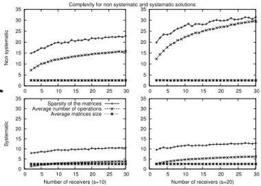
Complexity for non systematic and systematic solutions
0 5 10 15 20 25 30 35 0 5 10 15 20 25 30 Non systematic # 0 5 10 15 20 25 30 35 0 5 10 15 20 25 30 Systematic Number of receivers (s=10) #
Sparsity of the matrices Average number of operations Average matrices size
0 5 10 15 20 25 30 35 0 5 10 15 20 25 30 # 0 5 10 15 20 25 30 35 0 5 10 15 20 25 30 Number of receivers (s=20) #
Fig. 2. For s= 10 (on the left) or s = 20 (on the right), and P ER = 20%, all figures show the complexity for the receivers.
A. Average Matrix Size
We can observe from Fig. 2 that the average matrix size does not depend on s or the number of receivers. Indeed, the matrix’s size only depends on the number of packets which are lost, rather than the acknowledgements or the number of nodes involved. We can also observe that the size of the inverted matrices are very similar for both codes (for 30 receivers, the average size is 2.519 for the non-systematic and 2.522 for the systematic codes). We note that the non-systematic variant decodes more matrices, however a number of those have a size of one. This means that only one packet can be decoded after all the received packets have been subtracted from an encoded packet. However when a packet is lost, the systematic code needs to keep less packets in its buffer compared to the non-systematic code. For a (3, 4) code rate, this corresponds to one in every four packets for the systematic code, while the non systematic code stores all encoded (all received) packets in the matrix.
B. Sparsity of the Matrices
The sparsity of the matrix represents the average number of non-null elements in the matrix when inverted. This parameter provides an insight into how the matrix may be populated (is it empty or full). It is used to estimate the number of operations required to invert the matrix (in Section V-C) and it can also be used to better understand the size of the matrix.
First, it seems logical that when the number of receivers ors increases, the number of non-null elements in the matrix also increases. This is due to the increase of the encoding window size in the source (see Fig. 1), as each redundancy packet received is created from all the packets in the source buffer.
We can observe a lower bound of the variance of the size of the matrix by making the difference between the average
number of non-null elements and the matrix’ average size squared. In fact, the variancev verifies as:
v = [E(n2) − E(n)2] > [E(nnon null) − E(n)2]
wheren is the matrix’ size when inverted and nnon null, the
number of non-null elements in the matrix. Thus (note the values from Fig. 2) we can see that the lower bound of the variance is greater for the non-systematic codes than for the systematic ones. Furthermore, the variance is lower for the systematic case. Indeed, when any packet is lost, the non-systematic code inverts matrices of size one after the different subtractions when the systematic case does not have to decode the redundancy packets. Finally, when a packet is lost, the non-systematic code stores more encoded packets in its matrix than the systematic code, as they have to store every encoded packets after the lost one. This means one packet on four when the code is systematic but all of them in the other case.
C. The Average Number of Operations Per Unit of Time
As a criteria for the complexity, we choose the number of operations done per unit of time, rather than per matrix inversion. As the non-systematic code has to invert more matrices than the systematic code (e.g. it inverts matrices of size one even when all packets are received), the number of operations done per unit of time provides a better base for comparison of the two codes.
For both codes, it is logical that the average number of operations per unit of time increases whens and the number of receivers increase. The reason is twofold: as seen in Section V-B, the matrix’s sparsity value increases which implies that it is harder to invert the matrix. Furthermore, the source encoding window also increases, so when a receiver obtains a new encoded packet, it has to subtract more already received packets from it.
The main result of interest is a comparison of codes. We can observe that for all values ofs and any receiver number, the systematic code outperforms the non-systematic one. As seen previously, two factors define the number of operations which need to be performed by the codes: the matrix inversion and the number of subtractions needed when an encoded packet is received. The systematic code has superior results for both factors. We already noted that on average the matrix size for decoding packets is smaller for the systematic case, thus easier to invert, and the second point is that for the non-systematic code, all packets are encoded. Thus, every time a packet is received, the receiver has to perform a subtraction, as opposed to the systematic case, where this operation has to be done only when a repair packet is received. To illustrate the resulting impact, we can see that in the worst case (30 receivers and s = 20), the average number of operations needed for the non-systematic code is five times higher than for the non-systematic case.
VI. BUFFERSIZE ANDCOMPLEXITYANALYSISOVER A
BURSTYERASURECHANNEL
We now investigate the impact of bursty losses. We use a Gilbert-Elliot loss model, defined by a two states Markov chain
(consisting of a good and a bad state) as illustrated in Fig. 3. We choose an erasure burst length of 3. The parameters of this Markov chain are then calculated from the averageP ER chosen for the scenario. Knowing the average erasure burst length L and the well known formulas: P ER = p1/(1 + p1− p2) and L = 1/(1 − p2), thus p2 = 1 − 1/L and p1=
P ER/[L(1 − P ER)].
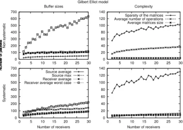
Fig. 4 shows the buffer sizes and the complexity fors = 20 andP ER = 20% for both codes.
Bad Channel State Good Channel State 1 − p2 p1 1 − p1 p 2
Fig. 3. The first-order two-state Markov chain representing the Gilbert-Elliott channel model
A. Buffer Sizes
As shown in Fig. 4, the bursty erasure channel results, not unexpectedly, in an increased buffer size requirements for both codes. However we can observe that this channel has a significant impact only on the receivers’ buffers. For the source, having a bursty channel results in a similar buffer sizes as previously observed for the non-systematic code, and the buffer slightly increases for the systematic case (the average number of packets is multiplied by 2 for the systematic code, but the worst case does not grow higher than 150 for both codes).
Concerning the receivers’ buffers, we can see that all the results are multiplied by at least a factor of two. However having a bursty channel has more impact on the non-systematic code than on the systematic one. We note that for 30 receivers, the average worst case has increased by a factor of 4 for the non-systematic code when using the Gilbert-Elliot model, which shows that on the average, there is always a receiver which has 620 packets in it’s buffer. For the systematic code, this value is equal to 210 packets, which is still three times higher than for the uniform erasure channel. Thus we can note that the Gilbert-Elliot model further highlights the differences between the codes already observed with the uniform loss model.
B. Complexity
As the erasures occur in bursts, on the average, more packets are lost before the decoding process, so the average matrix size and the number of non-null elements in the receiver matrices are higher than in the uniform erasure channel. The most relevant result is that, compared to the resulting values on the uniform erasure channel, the average number of operations per unit of time slightly increases for the non-systematic code, while it increases by a factor of two to three for the systematic variant. Therefore, although the Gilbert-Elliot model increases the complexity of the two codes, on the average, the systematic code will again require two to three times less operations than the non-systematic (e.g. it can be observed that for 30
receivers, the systematic code needs 15 operations per unit of time, while the non systematic needs 35).
Gilbert Elliot model
0 100 200 300 400 500 600 700 0 5 10 15 20 25 30 Non systematic Buffer sizes Number of packets 0 100 200 300 400 500 600 700 0 5 10 15 20 25 30 Systematic Number of receivers Number of packets Source average Source max Receiver average Receiver average worst case
0 20 40 60 80 100 120 140 0 5 10 15 20 25 30 Complexity Number of packets
Sparsity of the matrices Average number of operations Average matrices size
0 20 40 60 80 100 120 140 0 5 10 15 20 25 30 Number of receivers Number of packets
Fig. 4. For s= 20 and P ER = 20% using a Gilbert-Elliot losses model with an erasure burst length of 3, for both codes, on the left are the curves for the different buffers’ sizes, on the right the complexities.
VII. CONCLUSION
We have presented an analysis of the implementation as-pects of two classes of on-the-fly coding schemes for mul-timedia multicast communications. We have shown that the systematic approach has lower requirements in regards to the memory footprint and computation complexity of the receivers, thereby making it better suited for mobile devices. These points are crucial in the context of deployment of such schemes for IPTV or multimedia communications in mobile environments. In future work, we plan to progress the implementation of this scheme and to consider the feasibility of a reliable multicast protocol based on such a mechanism.
REFERENCES
[1] E. Martinian and C.-E. Sunberg, “Burst erasure correction codes with low decoding delay,” IEEE Trans. on Information Theory, vol. 50, no. 10, 2004.
[2] J. K. Sundararajan, D. Shah, and M. M´edard, “ARQ for network coding,” in IEEE ISIT, 2008.
[3] P.-U. Tournoux, E. Lochin, J. Lacan, A. Bouabdallah, and V. Roca, “On-the-fly erasure coding for real-time video applications,” IEEE Trans. on
Multimedia, vol. 13, no. 4, Aug. 2011.
[4] R. G. Gallager, “Low-density parity-check codes,” IEEE Trans. on
Information Theory, 1963.
[5] L. Rizzo, “Effective erasure codes for reliable computer communication protocols,” SIGCOMM Comput. Commun. Rev., vol. 27, pp. 24–36, April 1997.
[6] M. Arai, A. Yamamoto, A. Yamaguchi, S. Fukumoto, and K. Iwasaki, “Analysis of using convolutional codes to recover packet losses over burst erasure channels,” in IEEE PRDC, 2001.
[7] S. Puducheri and T. Fuja, “Coding versus feedback: Hybrid arq protocols for the packet erasure channel,” in IEEE ISIT, 2010.
[8] M. Luby, “LT codes,” in IEEE FOCS, 2002.
[9] A. Shokrollahi, “Raptor codes,” IEEE/ACM Trans. on Networking, vol. 14, Jun. 2006.
[10] J. K. Sundararajan, D. Shah, M. M´edard, M. Mitzenmacher, and J. ao Barros, “Network coding meets tcp.” in IEEE INFOCOM, 2009. [11] A. Soro, M. Cunche, J. Lacan, and V. Roca, “Erasure codes with a
banded structure for hybrid iterative-ml decoding,” in IEEE
![Table I illustrates the difference between the on-the-fly coding schemes proposed in [10] and [3].](https://thumb-eu.123doks.com/thumbv2/123doknet/3625426.106580/3.918.501.819.80.243/table-i-illustrates-difference-fly-coding-schemes-proposed.webp)