Performance evaluation of non Markovian stochastic discrete event systems - A new approach

PERFORMANCE EVALUATION OF NON MARKOVIAN STOCHASTIC DISCRETE EVENT SYSTEMS - A NEW

APPROACH

Serge Haddad, Lynda Mokdad ∗,1Patrice Moreaux ∗∗,1

∗_{LAMSADE, UMR CNRS 7024, Université Paris Dauphine,}

Place du Maréchal de Lattre de Tassigny, 75775 PARIS, FRANCE

∗∗_{LAMSADE & CReSTIC, Université de Reims}

Champagne-Ardenne, REIMS, FRANCE

Abstract In this work, we address the problem of transient and steady-state analysis of a stochastic discrete event system which includes non Markovian distributions with a finite support. Rather than computing an approximate distribution of the model (as done in the previous methods), we develop an exact analysis of an approximate model. The design of this method leads to a uniform handling for the computation of the transient and steady-state behaviour of the model. We have evaluated our method on a standard benchmark (the queuing model M/D/S/K). Our results demonstrate that: in most of the cases the

solution of the approximate model converges quickly to the solution of the exact model, in the difficult cases (e.g. an heavy load on the queue) our method is more robust than the previous ones.

Keywords: Discrete event systems, Stochastic processes, Markovian processes, Periodic processes, Uniformization

1. INTRODUCTION

The transient and steady-state analysis of Markovian discrete event systems is now well established with numerous tools at the disposal of the modellers. The main open issue is the reduction of the space com-plexity induced by this analysis. However in a re-alistic system, the distribution of the occurrence (or the duration) of some events can not be described by a exponential law (e.g. the triggering of a time-out). Theoretically any “reasonable” distribution is approx-imated by a phase-type distribution enabling again a Markovian analysis (Cox 1955b). Unfortunately the continuous time Markov chain (CTMC) associated to this approximation is so huge that it forbids its analy-sis (indeed even its construction). Such a phenomenon often occurs when the non exponential distribution has

1 _{{haddad,mokdad,moreaux}@lamsade.dauphine.fr}

a finite support (non null dirac, uniform, etc.); then a good phase-type approximation requires too much stages for its specification.

Hence the research has focused on alternative meth-ods. In the case of a single realization of a non Marko-vian distribution at any time, successful methods have been proposed (German et al. 1995) both for the tran-sient and steady state analysis. Let us cite, for in-stance, the method of supplementary variables (Cox 1955a, German and Lindemann 1994) or the method of the subordinated Markov chains (Ajmone Marsan and Chiola 1987).

The general case (i.e. simultaneous multiple realiza-tions of such distriburealiza-tions) is more intricate. The method of supplementary variables is still theoreti-cally applicable but the required space and the com-putation time limit its use to very small examples. An

alternative approach is described for non null Dirac distributions in (Lindemann and Schedler 1996). The stochastic process is observed at periodic moments of time ({i∆| i ∈ IN}) and this new process is

ex-pressed by a system of integro-differential equations and solved numerically. The steady-state distributions of these processes are identical and, with another com-putation, one obtains the transient distribution of the original process from some transient distribution of the transformed process. This method has been im-plemented in the DSPNexpress tool (Lindemann et al. 1999).

Here we propose to define an approximate model on which we perform an exact analysis. Let us first de-scribe the kind of model we will analyse: its behaviour is described by a CTMC, a discrete time Markov chain (DTMC) and a time interval (say∆). During an inter-val(i∆, (i + 1)∆) the behaviour is driven by the CTMC and at an instant i∆a untimed probabilistic change of state is processed according to the DTMC.

Now we describe how we obtain such a model from a general model with non Markovian finite support distributions. At first, we transform such a distribu-tion into a discrete distribudistribu-tion concentrated on the instants i∆ included in the support. This step can be done numerically in a straightforward way from the distribution function. So we will not develop it in the remaining paper. Let us note that ∆seems to be the approximation parameter but a better parameter is the ratio between∆and the size of the support (moreover this indicator is the key factor for the complexity of our analysis).

In the approximate process, the Markovian events oc-cur during the intervals(i∆, (i + 1)∆) and their logical occurrence is specified within the CTMC. Let us note that this is not an approximation since the set{i∆| i ∈

IN} has a null measure. Non Markovian events always

occur in {i∆| i ∈ IN}. Let us describe how they are

scheduled. When a non Markovian event is enabled in an interval (i∆, (i + 1)∆) due to the occurrence of a Markovian event then its approximate distribution is interpreted as the number of points i∆that must be met before its occurrence. Here we can choose whether we count the next point (an under-evaluation) or not (i.e. an overestimation). The impact of this choice will be discussed later. Thus the residual number of points to be met is included in the state. At any moment i∆, the current residual numbers are decreased. If some residues are null then the corresponding events occur with possibly some probabilistic choice in case of conflicts. The occurrence of these events may enable new non Markovian events. Such events are handled similarly except that the next point is always counted since now it corresponds to a complete interval. This process is not exactly ergodic since the steady-state distribution depends on the relative position w.r.t. the points i∆. The transient analysis is done by suc-cessively computing the state distribution at the

in-stants ∆, 2∆, . . . applying a transient analysis of the CTMC during an interval ∆ (via the uniformization technique (Gross and Miller 1984)) followed by a “step” of the DTMC. In order to smooth the effect of the discretization, we average the distribution on the last interval (with a variant of the uniformization). For the state analysis, one computes the steady-state distribution at the instants i∆ and then starting from this distribution, one averages the steady-state distribution upon an interval.

The balance of the paper is the following one. In section 2 we present our approach. Section 3 reports evaluations of the method applied to a first model. At last, we conclude and give indications on future developments of our work.

2. A NEW APPROXIMATE METHOD 2.1 Definition of the approximate process

As discussed in the introduction, we choose a time interval ∆. We approximate the original stochastic process X with the process Y . Roughly speaking, the approximation is related to the non Markovian events which can only occur at times th= h∆. The impact

of this approximation will be evaluated in the next section.

We then study the evolution of the stochastic process Y in each interval(th,th+1) and during the state changes

at time th. We denote by th− (th+) the "time" before

(after) the state change in th.

The process Y is defined by two components:

• the subordinated process in (th,th+1) associated

to states at t_h+records only exponential events. It is then a CTMC defined by its generator Q.

• the state changes at thare defined by a stochastic matrix P[i, j] = Pr(X(h∆+) = j | X(h∆−) = i).

Thus Y is fully defined by its initial probability vector

π(0) and the matrices (P, Q). These three components

depends obviously on ∆ since for instance the state space includes the residual number of instants.

2.2 Transient analysis

Let π(h∆+τ) the probability vector of the process Y

at time h∆+τ. We have π(h∆+τ) = π(h∆+_)eQτ_for 0≤τ<∆, and π((h + 1)∆−) = π(h∆+)eQ∆_{, so that}

π((h + 1)∆+) = π(h∆+)eQ∆P and finally

π((h + 1)∆+) = π(0)(eQ∆P)h+1 (1)

Since we want to smooth the discretization effect, we define the approximate value π(a)(h∆) of πX(h∆) as the averaged value of the probabilities of the states of

Y in(th,th+1): π(a)(h∆) = 1

∆Rh(h+1)∆ ∆π(τ)dτ.

Using (1) we have then:

π(a)(h∆) = 1 ∆π(0) (eQ∆P)h ∆ Z 0 eQτdτ (2)

Finally, we are in general interested by performance measures defined on the states of the system, and not on the states of the stochastic process Y . Hence, all components of π(a)(t) corresponding to a given state

of the original system (i.e. when forgetting the residual numbers) are summed up to compute performance measures (see the example in section 3).

2.3 Steady-state analysis

We also set the approximate value π(a) of π as the averaged value of the steady-state probabilities of the states of Y over (th,th+1) since this steady-state

distribution depends on the relative position in the interval. If π(∆) is the steady-state distribution of the DTMC with initial distribution π(0) and transition

probabilities P(∆)= eQ∆_{P then} π(a)= 1 ∆π(∆) ∆ Z 0 eQτdτ (3)

By definition, π(∆)is the probability vector solution of

π= π.P(∆).

As in the transient case, all components of π(a) corre-sponding to a given state of the system are summed up to compute performance indices.

2.4 Numerical considerations

Formulae (2) and (3) for transient and steady-state probabilities involve vector-matrix products with pos-sibly very large matrices, either eQ∆or I(∆)=R∆

0 eQτdτ.

Moreover, it is well known that, although Q is gener-ally very sparse (see section 3 for an example), eQτ is not sparse (the “fill in” phenomenon). The usual approach to compute these matrices is then based on series expansion and numerical summation until a re-quired precision level. We have implemented a similar algorithm to compute the vector-matrix products di-rectly using the series expansions.

When we need eQτ we follows the uniformization approach (Stewart 1994). If P(u) = I + 1_uQ is the

uniformized matrix of Q with rate u> maxi{|qii|}, we

have eQτ=

∑

∑

Using an integration by part, Ik= R∆ 0 e−ut (ut) k k! dt may be expressed as I_k= −e −u∆_(u∆)k uk! + Ik−1 for k≥ 1 Hence, I0= − e−u∆ u + 1 u Ik= 1 u " 1− e−u∆ h=k

∑

∑

∑

As for e(Q∆), we only need I(∆) through products

1

∆.W.I(∆). Hence we compute these products

itera-tively to avoid the fill in. An analogous approach was used in (German 2001) for steady-state solution of De-terministic Stochastic Petri Nets (DSPN) but restricted to one deterministic event at any given time.

3. APPLICATION: THE M/D/S/K QUEUE

In order to evaluate it, we apply our method to the M/D/S/K queue (Poisson arrival with rate λ, deter-ministic service time with duration D, S servers and finite capacity K). The M/D/S/K queue is an

inter-esting case study for several reasons. First, this model presents multiple non exponential concurrent activi-ties (for 1< S ≤ K). Second, no analytical results are

available for the transient or even steady-state distri-bution of the queue length or other performance in-dices of this queueing model (for S> 1) unless S = K.

It is thus significant to get quickly an approximation of these performance indices. Finally, due to the sim-plicity of the underlying process, we are able to easily compare our results with existing analytical or numer-ical tools for S≤ 2.

3.1 The approximate process

Let us recall that our approximation lies in the fact that non exponential events, i.e. the ends of (deterministic) service are recorded only at times h∆. For ease of notation, we set∆= D/n so that n will be the indicator

of the precision of the approximation in the rest of the paper.

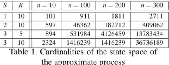
S K n= 10 n= 100 n= 200 n= 300

1 10 101 911 1811 2711

2 10 597 46362 182712 409062 3 5 894 531984 4126459 13783434 3 10 2324 1416239 1416239 36736189

Table 1. Cardinalities of the state space of the approximate process

When we take into account these events, we may choose between two approximate strategies: either un-derestimate the (new) requested service time, choos-ing n∆ (“low” (L) choice) or in contrast overesti-mate this service time, choosing(n + 1)∆(“high” (H) choice). This leads to two series of parameters and approximate distributions that we denote by L or H superscript or∗ for any of them; n(∗)stands for n or n+ 1.

A state of the model is thenhc, xi where

• c is the number of clients in the queue with

0≤ c ≤ K;

• x = (x1, x2, . . . , xmin(c,S)) is the tuple of service

states of each served client with n(∗)≥ x1≥ x2≥ . . . ≥ xmin(c,S).

The stateh0, −i corresponds to an empty queue and

is the initial state of the system. States are ordered w.r.t. a kind of lexicographic order: the first state is

h0, −i and hc, xi < hc′, x′i iff c < c′ or c= c′ and x= (x1, . . . , xu) ≤ x′= (x′₁, . . . , x′v) i.e. u < v or u = v

and there is w such that xi= x′ifor all i< w and xw< x′w

(lexical order between vectors).

There is no simple closed form for the cardinality of these state-spaces Sn(L) and S(H)n . They are obviously

bounded by (K + 1)(n + 1)S _{but this is a very high}

bound. Table 1 gives the values of S(H)n for some

parameters.

In the M/D/S/K case, the Q matrix defined in

sec-tion 2 is very simple (in fact upper-triangular). From each state hc, xi (with c < K) the only exponential

event is the Poisson arrival of a new client (rate λ), thus

hc′, x′i =½ hc + 1, xi (S ≤ c < K) hc + 1, (n(∗)_{x1, . . . , x}

min(c,S))i (c < S)

If c= K there is no transition from hc, xi.

The P matrix records state changes due to non expo-nential events at times h∆. It has one only non null term per row (with c> 0) corresponding to decrease of

remaining service times and possible ends of service followed by starts of service of waiting clients (P is lower-triangular). Let e= |{xi| xi= 1}| be the number

of servers which will end their service at next h∆time in s= hc, xi. Then b = max(min(e, c − S), 0) is the

number of servers that will start a new service at h∆ from s (such a server may have been busy or idle before h∆). Then, fromhc, xi, there is a transition with

probability 1 tohc′_{, x}′_{i equal to}

hc − e, (n(∗), . . . , n(∗), x1− 1, . . . , xmin(c,S)−e− 1)i

with b occurrences of n(∗)on the left side of x′. There is no transition fromh0, −i (P[1, 1] = 0.0).

3.2 Solving the approximate process

We compute approximate distributions (see section 2) for increasing values of n until they are as close as the required precision. Transient distributions are computed for discrete time horizons h∆. In all the paper, we use the L1 normk π2− π2k=∑i|π1[i] − π2[i]| to compare two probability distributions π1and π₂.

Let us denote πn(L)(h) (resp. π(H)n (h)) the distribution

at time h∆ computed for a given elementary time step ∆= D/n by taking approximate service delay

n∆ (resp. (n + 1)∆). We observed that each of the sequences (π(L)n (h))n and (πn(H)(h))n converges to π(L)(h) and π(H)(h) but that k π_n(L)(h) − π_n(H)(h) k

does not necessarily converge to 0. Moreover, several comparisons showed that depending on the parame-ters, one of the two sequences converges faster than the other and also that one of the two limits is closer to the exact distribution than the other, but we did not found any clear rule to choose between the two approximate distributions. These behaviours lead us to define the approximate distribution for n as a weighed sum of πn(L)(h) and πn(H)(h) based on their respective

convergence rate: π(a)_n (h) = 1 dn(L)+ dn(H) ³ dn(L)π(L)_n (h) + d_n(H)π_n(H)(h) ´ with dn(∗) = 1 kπ(∗)_n (h)−π(∗) n′(h)k

. and n′ is the previous value used in the iterative approximation process. The steady-state approximate distribution is defined simi-larly.

For a given n, in both transient and steady-state cases, we first compute the matrices P(L)n ,P(H)n , Q(L)n ,Q(H)n .

The initial probability vector is defined as πn(0)[1] =

1 and πn(0)[ j] = 0 for all j > 1.

In the transient case (see (2)) we first compute the vector V=_∆1πn(0) µ eQ(∗)n ∆_(P(∗) n )h ¶

then the product

π(∗)_n (h) = V.

∆

Z

0

eQ(∗)n τ_dτ

Note that we never compute neither eQ(∗)n ∆ _{nor the}

integral matrices to avoid fill in.

In the steady-state case (see (3)), we first compute the solution πn(∗,∆) of π = π.Pn(∗,∆) with P(∗,n ∆) =

time horizon

ρ 10D 50D 100D

0.1 40 - 10−4 40 - 10−4 40 - 10−4 1.0 120 - 10−4 140 - 10−3 150 - 10−3 10.0 110 - N/A 145 - N/A 150 - N/A

Table 2. Minimal n for d≤ 10−3_and

preci-sion of the approximation for S= 2, K = 5

eQ(∗)n ∆_P(∗)

n using an iterative method. Then we

com-pute the product

π(∗)_n = 1 ∆π_n(∗,∆) ∆ Z 0 eQ(∗)n τ_dτ

From the two vectors πn(L)(h), π(H)n (h) (or their

steady-state versions) we derive π(a)n (h) and we iterate

(in-creasing n by some step value) until k πn(a)(h) − π(a)

(n′₎(h) k reaches a given precision levelε. 3.3 Numerical results

We did several comparisons to validate our method and study its behaviour w.r.t. to the convergence and the precision of the approximation. All our compu-tations were done on a Pentium-PC 2.6Ghz, 512MB, with Scilab 2.7.2 (INRIA 2002) under SuSE Linux. For all these measures, we have fixedε= 10−3_{, K=}

5, 10. As we will show, the behaviour of the

imple-mentation depends heavily on the ratio ρ =λD/S

which can be seen as the load indicator of the queue. Hence we have fixedλ= 1.0 in all experiments and we

varyρin{0.1, 0.5, 1.0, 5.0, 10.0}, that is to say from

a very low to a very high loaded system. For S= 1

we used several tools, mainly based on SPN: DSP-Nexpres (Lindemann 2003), GreatSPN (P.E. Group 2002), SPNica and TimeNET (German 2000). We also developed an exact solution based on the sup-plementary variable approach (Cox 1955a, German and Lindemann 1994) and we compared our approx-imation with this method too. For S = 2, we used

DSPNepress-NG, the last version of DSPNexpress, the only analytical tool available to the best of our knowledge for two concurrent deterministic events (see (Lindemann 1998, Lindemann et al. 2000) for a detailed presentation). We do not report detailed results do to space limitation. We simply indicate the main trends we have observed.

3.3.1. Transient analysis In the transient case, we did computations for time horizons t= 10D, 50D and

100D which correspond to h= 10n, 50n and 100n for a

given value of n (which varies during the computation of the approximation). To evaluate the convergence of the approximation, we computed the minimal n such that d =k π(a)n (h) − π(a)_(n−1)(h) k≤ 10−3. Results for

S= 2 are given in Table 2. In all cases, the minimal

n was between 100 and 200 and is increasing slowly

with t. For K = 10, we have observed however that

for ρ≫ 1, the variation on πn(a)(h) first decreases

(n≤ 300) but then increased with n. This indicates

clearly that for large n, numerical computations be-come unstable. In all cases, we observed a difference lower than 10−3 between our approximation and the result given by DSPNexpress-NG.

3.3.2. Steady-state analysis We did the same ex-periments for the steady-state case. As suspected by the transient analysis, the required n to reach a fixed precision depends largely onρ. In fact, since we force the end of service time at n∆ only, our method pro-vides an almost exact result when either the servers are almost always idle (ρ≪ 1) or busy (ρ≫ 1). We

recognize this behaviour both in the higher values of n and the lower precision. This property of our method is also illustrated by the results (not reported here due to lack of space) for the special case S= K for

which the exact result is known to be equal to the M/M/S/S queue. In this infinite server case, every

end of service is immediately followed by a beginning of service when the system is heavily loaded. In these cases we have obtained small values of n to get the approximation. In contrast, forρ≈ 1, the convergence

is slow (n≈ 200 − 300) and the approximation is not

so good (precision=10−3). For K= 5 (resp. K = 10)

and ρ= 4.5 (resp. ρ> 1.75), we have noticed that

DSPNexpress-NG gives erroneous probabilities (i.e. negative values) so that we could not compare our result with an “exact” numerical value.

4. CONCLUSIONS AND PERSPECTIVES We have presented a new approximate method for stochastic processes with multiple non Markovian concurrent activities. Contrary to the other methods, we have approximated the model and applied an exact method rather than the opposite way to do. The key factor for the quality of this approximation is that the occurrence of Markovian events are not approxi-mated as it would be in a naive discretization process. Furthermore, the design of its analysis is based on robust numerical methods (i.e. uniformization) and the steady-state and transient cases are handled similarly. The examples have shown that our method is robust. For instance when analysing an heavy queue the pre-cision is still correct (i.e. 10−3whereas DSPNexpress-NG (a very efficient tool in general) gives negative probabilities!

We are currently extending our method in two direc-tions. The first one is to adapt the approach to models exhibiting very different durations (stiff models). In such cases, the determination of ∆ uniquely based on the smallest deterministic delay would lead to in-tractable matrices and vectors.

The second extension is related to the introduction of tensorial expressions for the matrices in order to manage the space complexity associated to systems with many non Markovian concurrent activities.

Acknowledgments We would like to thank the

au-thors of the different solvers we have used for provid-ing us the last version of their software.

REFERENCES

Ajmone Marsan, M. and G. Chiola (1987). On Petri nets with deterministic and exponentially dis-tributed firing times. In: Advances in Petri Nets 1987 (G. Rozenberg, Ed.). pp. 132–145. Number 266 In: LNCS. Springer–Verlag.

Cox, D. R. (1955a). The analysis of non-Markov stochastic processes by the inclusion of supple-mentary variables. Proc. Cambridge Philosophi-cal Society (Math. and Phys. Sciences) 51, 433– 441.

Cox, D. R. (1955b). A use of complex probabilities in the theory of stochastic processes. Proc. Cam-bridge Philosophical Society pp. 313–319. German, R. (2000). Performance analysis of

commu-nication systems. John Wiley & Sons,Ltd. Chich-ester, England.

German, R. (2001). Iterative analysis of Markov regenerative models. Performance Evaluation

44, 51–72.

German, R. and C. Lindemann (1994). Analysis of stochastic Petri nets by the method of supplemen-tary variables. Performance Evaluation 20(1– 3), 317–335. special issue: Peformance’93. German, R., D. Logothesis and K.S. Trivedi (1995).

Tran-sient analysis of Markov regenerative stochastic Petri nets: A comparison of approaches. In: Proc. of the 6th International Workshop on Petri Nets and Performance Models. IEEE Computer Soci-ety Press. Durham, NC, USA. pp. 103–112. Gross, D. and D.R. Miller (1984). The randomization

technique as a modeling tool an solution proce-dure for transient markov processes. Operations Research 32(2), 343–361.

INRIA (2002). Scilab home page:

http://www.scilab.org.

Lindemann, C. (1998). Performance Modelling with Deterministic and Stochastic Petri Nets. John Wi-ley & Sons.

Lindemann, C. (2003). DSPNexpress home page:

http://www.dspnexpress.de. .

Lindemann, C., a. Klemm, M. Lohmann and O. Wal-horst (2000). Quantitative system evaluation with DSPNexpress 2000. In: Proc. of the 2nd Int. Workshop on Software and Performance (WOSP). Ottawa, canada. pp. 12–17.

Lindemann, C., A. Reuys and A. Thümmler (1999). DSPNexpress 2.000 performance and depend-ability modeling environment. In: Proc. of the

29th Int. Symp. on Fault Tolerant Computing. Madison, Wisconsin.

Lindemann, C. and G.S. Schedler (1996). Numerical analysis of deterministic and stochastic Petri nets with concurrent deterministic transitions. Perfor-mance Evaluation 27–28, 576–582. special issue: Proc. of PERFORMANCE’96.

P.E. Group (2002). GreatSPN home page:

http://www.di.unito.it/∼greatspn.

Stewart, W. J. (1994). Introduction to the numerical solution of Markov chains. Princeton University Press, USA.