Time-gated detection of near-infrared emitting quantum dots for in vivo cell tracking

HAL Id: tel-01083824

https://pastel.archives-ouvertes.fr/tel-01083824

Submitted on 18 Nov 2014

HAL is a multi-disciplinary open access archive for the deposit and dissemination of sci-entific research documents, whether they are pub-lished or not. The documents may come from teaching and research institutions in France or

L’archive ouverte pluridisciplinaire HAL, est destinée au dépôt et à la diffusion de documents scientifiques de niveau recherche, publiés ou non, émanant des établissements d’enseignement et de recherche français ou étrangers, des laboratoires

dots for in vivo cell tracking

Sophie Bouccara

To cite this version:

Sophie Bouccara. Time-gated detection of near-infrared emitting quantum dots for in vivo cell track-ing. Life Sciences [q-bio]. Université Paris Diderot, 2014. English. �tel-01083824�

présentée par

Sophie BOUCCARA

pour l’obtention du grade de

Docteur de l’UNIVERSITÉ PARIS DIDEROT (Paris 7)

ÉCOLE DOCTORALE FRONTIÈRE DU VIVANT

Specialité: Physique du vivant

Laboratoire de Physique et d’Étude des Matériaux

Time-gated detection of near-infrared

emitting quantum dots for in vivo cell

tracking in small animals

soutenue le 22 septembre 2014

devant le jury constitué de :

Mme. Sandrine LÉVÊQUE-FORT Rapporteur

M. Stéphane PETOUD Rapporteur

Mme. Geneviève BOURG-HECKLY Examinateur

M. Frédéric DUCONGÉ Examinateur

M. François TREUSSART Examinateur

Remerciements

Je pense que la partie “Remerciements” est la partie la plus difficile à écrire dans un manuscrit de thèse. Je remercie tous ceux qui m’ont permis de mener cette thèse en espérant n’oublier personne.

J’aimerais commencer par remercier les membres de mon jury. Merci à San-drine Lévêque-Fort et Stéphane Petoud d’avoir accepté de rapporter ma thèse. Je remercie Sandrine Lévêque-Fort de m’avoir suivie tout au long de ma thèse, merci pour les discussions autours du time-gated et le coaching profession-nel dans le bus d’ELMI. Merci Stéphane Petoud d’avoir trouvé autant d’intérêt au travail que j’ai fourni. Je remercie aussi Frédéric Ducongé qui m’a égale-ment suivie tout au long de ma thèse. Je te remercie pour les discussions que nous avons pu avoir et surtout pour ton expertise en biologie durant les “Thesis Advisory Committees”. Merci à Paul French d’être venu de Londres pour assister à ma soutenance et merci pour les échanges que nous avons pu avoir. Merci à François Treussart d’avoir accepté d’examiner ma thèse et merci pour les remarques sci-entifiques intéressantes que vous avez fournies le jour de la soutenance. Un merci particulier à la présidente du jury Geneviève Bourg-Heckly qui m’a donné le goût de la recherche biomédicale et qui a été pour moi un modèle scientifique tout au long de mes études universitaires.

Ma thèse n’aurait pas été possible sans Alexandra Fragola. Merci Alexan-dra d’avoir eu confiance en moi et d’avoir pensé ce sujet qui m’a tant passionnée. C’est grâce à toi que j’ai pu découvrir ce laboratoire et cet environnement scien-tifique que j’ai adoré. Merci pour les discussions scienscien-tifiques et le rôle de maman que tu as si bien tenu pendant ces dernières années. Merci à Vincent Loriette, mon directeur de thèse pour qui l’optique n’a aucun secret. Merci d’avoir accepté de me prendre en thèse alors que tu ne croyais pas au sujet. J’espère que ce sujet t’a donné envie de commencer une carrière en synthèse de quantum dots. Merci à Thomas Ponspour ta présence et ton excellence scientifique. J’ai eu énormément

manquer. Merci à Nicolas Lequeux pour ton savoir en matière de ligands, ton sens de l’humour et tes critiques sur ma façon de m’habiller qui m’ont, dans le fond, souvent amusées. Merci à Sandrine Ithurria Lhuillier pour nos discussions de commérage, j’ai jamais vu une commère comme toi. Merci à Benoît Dubertret de m’avoir accueillie dans son équipe. Merci à Ivan Maksimovic pour ton humour sarcastique qui m’a fait tant rire. Merci à Xiangzhen Xu pour les heures passées au TEM.

J’aimerais remercier maintenant mes co-bureaux. Je dois bien sûr commencer par mon binôme de thèse Gary Sitbon sans qui ma thèse n’aurait pas été aussi belle. Merci Gary d’avoir supporté mon stress, mes humeurs, mon bordel et merci d’être devenu l’ami que tu es. Tu es quelqu’un de génial ne l’oublie pas s’il te plait. Merci Emerson Giovanelli pour tes conseils et ton excellente pédagogie en chimie, heureusement que tu es patient. Merci pour tes gentilles attentions et pour ton soutien à San Francisco. Je ne te souhaite que des bonnes choses. Merci Michel Nasilowski alias Mich Mich. Tu es quelqu’un d’adorable, ne te laisse pas marcher dessus et ne doute pas de toi. Vous avez été tous les trois d’excellents co-bureaux pendant ces trois années je vous remercie grandement pour ces beaux moments qu’on a partagés.

J’aimerais remercier tous les anciens de l’équipe qui m’ont rapidement manqué après leur départ :

• Eleonora Muro : j’ai été triste qu’on se croise si peu au labo et j’aurais adoré maniper avec toi. Nous nous sommes tout de suite bien entendues et nous avons eu tellement de fous rires ensemble. Heureusement, c’est parti pour continuer.

• Clémentine Javaux : merci pour ton caractère et ta générosité. Tu nous reçois toujours tellement bien. Tu es une fille déterminée et une amie super.

• Pierre Vermeulen : mon frère de thèse. J’ai été complètement perdue quand tu es parti et tu m’as beaucoup manqué dans les salles d’optique que j’arpentais seule. Merci d’être venu m’écouter j’ai été très touchée.

• Benoît Mahler : merci pour les fous rires inter-bureaux et les clopes qu’on fumait ensemble en cachette. Tu es un bon vivant et ton rire nous a vite manqué au labo.

partie ça a vite été l’anarchie. Tu es une grande scientifique je te souhaite de réussir.

• Cécile Bouet : merci ma coach sportive. Tu m’as donné le goût de la course et ce n’était pas gagné. Merci pour ta gentillesse et ta douceur.

• Mickaël Tessier : merci pour ton aide lors de la préparation des TD et pour tous ces vendredis soirs qu’on a passé à discuter.

• Arjen Dijksman : merci pour tes conseils lorsque je suis arrivée au labora-toire.

• Botao Ji : Merci Botao d’avoir partagé ces trois années de thèse avec moi et bon courage pour la suite.

Je remercie les membres de Nextdot, la start up du labo. Je remercie Brice Nadal pour sa gentillesse et son altruisme. Merci pour ton aide et ta présence durant ces trois années dans les moments joyeux comme les plus tristes. Je remercie Chloé Grazon pour sa spontanéité, ses rires qui mettent de l’ambiance au labo et ses discussions “girly-girly” . Je remercie Hadrien Heuclin pour son aide précieuse pendant la rédaction, Emmanuel Lhuillier pour son art à déplaire et Martin Guilloux pour ses remarques de business man qui donnent une autre dimension aux discussions. Merci aussi à la bella Silvia Pedetti pour son sourire et son art de la fête, que de bons souvenirs à Copenhague.

Merci ensuite à Aurore Bournigault ma stagiaire préférée, Aude Buffard la jolie rousse (sois forte), Marianna Tasso l’argentine grâce à qui j’ai pratiqué (un peu) mon espagnol, Piernicola Spinicelli l’un des meilleurs cuisiniers de Paris, Anusuya Banerjee pour sa douceur, Adrien Robin le Lincoln de l’ESPCI, Patrick Hease le jeune paresseux (ne te laisse pas faire par les autres), Fatima, Céline et Laura les nouvelles à qui je souhaite de passer d’excellents moments dans l’équipe.

Je remercie les membres du laboratoire de Neurobiologie avec qui j’ai travaillé : Sophie Pezetet Zsolt Lenkei pour les manips sur souris, Anne Simon pour la culture cellulaire et Delphine Ladarré pour son soutien pendant la rédaction.

Je remercie également Jérôme Lesueur et Ricardo Lobo les directeurs du LPEM pendant ma thèse. Merci à Sophie Demonchaux pour sa disponibilité et ses conseils avisés pendant ces trois années, Marie-Claude Theme pour sa

du LPEM, et en particulier Maxime Malnou et Simon Hurand.

Je remercie aussi mon école doctorale, FDV, qui m’a permis de rencontrer un grand nombre de scientifiques de qualité. Je remercie également les Laboratoires Servier d’avoir financé ma thèse ainsi que de m’avoir donné les moyens de participer à un nombre incalculable de conférences. Un merci particulier à Olivier Nosjean pour tous tes conseils et la confiance que tu m’as accordée pendant ces trois années. Enfin j’aimerais remercier tous mes amis de Vanves, de Montréal et d’ailleurs qui sont venus me voir le jour de la soutenance. Vous m’avez donné beaucoup de force et de courage. Merci également aux membres de Transapi, association dans laquelle je me suis investie en thèse et dont le projet est génial. Je remercie bien sûr ma famille, mes parents pour leur soutien, leur amour et leur confiance depuis toujours, mes soeurs Boubou et Bubu que j’aime fort et ma tante Michèle toujours prête à me faire plaisir. Pour finir j’aimerais remercier Samuel Peillon pour m’avoir supporté pendant la thèse, je sais que ce n’était pas facile tous les jours. Merci mon Sam de ta patience et de ton soutien, sans toi j’aurais pu perdre pied.

Contents

Remerciements iii

Introduction 1

I In vivo cell tracking: state of the art 3

I.1 Cell tracking techniques . . . 8

I.1.1 PET . . . 8

I.1.2 Magnetic Resonance Imaging . . . 9

I.1.3 Bioluminescence imaging . . . 9

I.1.4 Fluorescence microscopy . . . 10

I.1.5 Summary of the different imaging techniques characteristics . 13 I.2 Fluorescence microscopy limitations . . . 13

I.2.1 Visible light scattering and absorption . . . 13

I.2.2 Tissue autofluorescence . . . 14

I.3 Solution proposed to reduce the autofluorescence signal . . . 18

I.3.1 Time-gated detection coupled to long lifetime nanoprobes . . . 19

I.3.2 Current applications of time-gated detection for autofluores-cence rejection . . . 19

I.4 Conclusion . . . 26

II Near-infrared-emitting quantum dots for cell labelling 29 II.1 Introduction . . . 30

II.2 Zn-Cu-In-Se cores . . . 33

II.2.1 Synthesis . . . 33

II.2.2 Structural properties . . . 36

II.3 ZnS shell . . . 40

II.3.1 Synthesis . . . 41

II.4 Influence of trap states on the optical properties . . . 45

II.5 QDs as probes for biological applications . . . 48

II.5.1 Solubilization in water . . . 48

II.5.2 Cell labelling technique . . . 55

II.5.3 QDs toxicity . . . 59

II.6 Conclusion . . . 66

III Optical set-up, characterization and operation modes 67 III.1 Introduction . . . 68

III.2 Experimental set up . . . 70

III.2.1 Description . . . 70

III.2.2 Operation of the intensifier . . . 70

III.2.3 Set up flexibility . . . 72

III.3 Set up characterization . . . 73

III.3.1 Spatial resolution . . . 73

III.3.2 Noise sources . . . 78

III.3.3 Influence of the noise signal on the signal-to-noise ratio (SNR) 82 III.3.4 Detection noise conclusion . . . 85

III.4 Fluorescence lifetime measurements . . . 86

III.4.1 Principle . . . 86

III.4.2 Influence on the gate width for the lifetime mesurements . . . 88

III.4.3 Measurements on QDs in different media and in the cell cyto-plasm with time . . . 89

III.5 Conclusion . . . 91

IV Time-gated detection for autofluorescence rejection 93 IV.1 Introduction . . . 94

IV.2 Short lifetime rejection . . . 96

IV.2.1 Description of the ratio R (τ, ∆) . . . 96

IV.2.2 Test with spatially separated short lifetime and long lifetime QD signals . . . 98

IV.2.3 Test in a real autofluorescent sample . . . 103

IV.2.4 Preliminary results for in vivo experiments . . . 105

IV.3 Determination of optimal values of the different parameters . . . 108

V.1 Synthesis of near-infrared-emitting quantum dots . . . 116

V.2 Solubilization in water: ligand exchange . . . 118

V.3 Electroporation of HeLa cells . . . 119

V.4 Chemical and biological products used . . . 120

V.4.1 Chemical products . . . 120

V.4.2 Chemical solvents . . . 120

V.4.3 Biological products . . . 120

V.4.4 Preparation of cell medium for HeLa cells . . . 121

V.4.5 Preparation of cell medium for A20 cells . . . 121

Conclusion 123 Appendix A : Vegard’s law and estimation of QDs concentration 137 A.1 Vegard’s law . . . 137

A.2 Estimation of the cores concentration . . . 138

A.3 Estimation of the core/shell nanocrystals concentration . . . 139

Appendix B : Set up characteristics 141 B.1 Optical set up components . . . 141

B.1.1 Filters properties . . . 141

B.1.2 High Rate Intensifier quantum efficiency . . . 142

Introduction

In the last decades, cancer therapies have become a large field of researches. Cell tracking techniques would allow a better understanding of the metastatic processes. Today, identifying the spread of cancer cells from a primary tumour to seed sec-ondary tumours in distant site, is one of the greatest challenges in cancer under-standing and treatments. It has been shown that only one in five patients will survive once diagnosed with metastases. For this reason, many researches in oncol-ogy have been developed to better diagnosing primary tumours and better detecting first metastases in order to implement new therapies.

In vivo detection of unique cell remains a challenge because few techniques are

sensitive enough to allow the detection of rare individual and isolated events. Pri-mary Intraocular Lymphoma is a lymphoma of the eye that creates brain metastases. The metastatic migration pathway of circulating tumour cells (CTC) from the eye to the brain is still unknown. A best knowledge about the CTC migration pathway should allow finding new therapies. Moreover, quantitative and kinetic CTC studies in an in vivo PIOL model would test the efficiency of different treatments. There-fore fluorescence microscopy that is very sensitive and allows detection of only a few probes, is a diagnostic adapted tool. Nevertheless its sensitivity is limited by two major factors. First, the low visible light penetration depth. In order to reduce this limitation there is a wavelength range where absorption and scattering by tissues are limited. This range of wavelengths goes from 680 to 900 nm. The other factor that limits the sensitivity is the tissue autofluorescence. Autofluorescence is the natural emission of photon-excited tissues. In order to reduce these two limitations, the flu-orescence signal peak wavelength of the nanoprobes should lie in an absorption and diffusion free region and should be distinguishable, either spectrally or temporally, from the autofluorescence background.

During my PhD thesis, I’ve worked on the synthesis of fluorescent nanoparticles with adapted optical properties for in vivo imaging. These fluorescent nanoprobes

should have an emission wavelength in the optical therapeutic window and should be bright, small and biocompatible. They also should have a long fluorescent lifetime to be coupled to a time-gated detection. Indeed, autofluorescence has a short fluo-rescence lifetime (<5 ns). By coupling long fluofluo-rescence lifetime with a time gated detection, we could enhance the sensitivity and reduce autofluorescence signal. I’ve also developed the optical set up to perform time-gated detection and have obtained promising preliminary in vivo results. The manuscript is divided in five chapters.

The FIRST CHAPTER is a state of the art of the different cell tracking tech-niques that have been developed and used in the last years. I will focus on our choice to work with optical microscopy and develop the different limitations we had to get ride of.

The SECOND CHAPTER describes the synthesis, characterisation of near-infrared long fluorescence lifetime quantum dots. I will report the protocol of water-solubilzation and the technique of cell labelling used in order to obtain massively loaded cells. I will also present some toxicity tests performed with our nanoprobes. The THIRD CHAPTER is a description and characterization of the optical set up I developed. As we want to detect few and rare cells, we have to be highly sensitive. I will present our set up behaviour regarding noise sources. I will also determine our imaging system spatial resolution.

The FOURTH CHAPTER is my results chapter. I will present how we have managed to enhance sensitivity by reducing autofluorescence signal. I will present three types of experiments from in vitro results to our last in vivo promising results. The FIFTH CHAPTER is a protocol chapter. I will list all chemical and biolog-ical products used for my experiments. I will also report the different protocols for the different steps of this project.

I

In vivo cell tracking is an interesting tool to understand many biological

pro-cesses. In tissue engineering, the ability to track implanted cells is essential to finely control the tissue monitoring and to direct tissue growth [1]. For immunotherapy that consists in administrating substances to induce an immune response, in vivo cell tracking could allow us to understand the molecular basis of immune cell biodis-tribution and trafficking [2]. Finally, tumour cell tracking can allow us to study their biodistribution and in vivo activity in order to improve our understanding of cancer development and metastatic processes. These examples of applications of in

vivo cell tracking require the detection of isolated cells, which still remains a

chal-lenge today. Some of these applications require the detection of few cells previously stained with a contrast agent.

The spread of cancer cells from a primary tumour to seed secondary tumours at distant sites, commonly called metastasis, is one of the greatest challenges in cancer treatment today. In 2011, the National Cancer Institute has published alarming data about the survival prognosis of patients diagnosed with metastases. Indeed, across all cancer types, only one in five patients diagnosed with metastatic cancer will survive more than 5 years (data from the National Cancer Institute in USA) [3]. It is crucial for the mechanisms of metastatic migration to be established because each step represents an opportunity for a new therapy. Moreover, tumour targeting for delivery treatments is also crucial [4]. Figure I.1 is a scheme of the different steps of metastasis. Briefly, tumour cells from the primary site break the epithelial cell barrier and clear a path for migration into the vasculature rich stroma. Cells are then introduced in the body bloodstream and reach a second host site. To proliferate in the secondary site, cancer cells release pro-inflammatory compounds and proteinases that induce growth factor releasing by their neighbours [5][6]. Here, tumour cells spread through the bloodstream but the lymphatic system is also a possible pathway. An other interesting challenge is to determine the migration pathway by detecting the tumour cells when leaving the original tumour site in order to reach another one. These type of cells are called circulating tumour cells (CTC).

Circulating tumour cells are spilled by primary tumours to invade other organs. In 1869 Thomas Ashworth, an Australian physician, after observing microscopically circulating tumour cells in the blood of a man with metastatic cancer, postulated that "cells identical with those of the cancer itself being seen in the blood" [8][9]. Then, researchers started to study this type of cancer cells and understood that the number of CTC can be a sensitive biomarker for tumour progression and metastasis

in some cases of cancers. In 2004, Cristofanilli et al. showed that the level of CTC can predict survival in metastatic breast cancer [10]. Therefore, the detection of CTC is useful for diagnosis and "staging" of cancers, to estimate the efficiency of treatments and to evaluate the presence of residual metastasis. However, the number of CTC in the blood or in lymphatic circulation is very low (few cells per mL). Therefore, the detection of CTC require a high sensitivity that could allow the detection of individual and isolated cells.

For my PhD project, we started a collaboration with Sylvain Fisson’s group in the Centre de Recherche des Cordeliers in Paris. His group works on the influence of the microenvironement in metastasis spread and one of the unsolved issue is the determination of the metastatic migration pathway for some cancers, such as the Primary IntraOcular Lymphoma. Primary intraOcular lymphoma (PIOL) is a high-grade non Hodgkin lymphoma: a cancer originating from white blood cells called lymphocytes. Most patients show non-specific visual symptoms and are often initially diagnosed with uveitis (inflammation of the uvea) or retinitis (inflammation of the retina). Unfortunately, the definitive diagnosis is obtained when clinical symptoms of cerebral lymphoma appear [11]. Indeed, it has been shown that up to 80% of the patients who initially present ocular lymphoma will develop cerebral lymphoma [11][12][13][14][15]. A better understanding and prevent of the spread of tumour cells to the brain could improve the survival diagnosis. However, the migration pathways from the eye to the brain are still unknown. There are two suspected pathways: via the lymphatic system or via the bloodstream. In 2007, the group of Sylvain Fisson developed a murine model in order to study the immune microenvironmenent which is known to be crucial in controlling tumour growth and maintenance [16]. In this model, they implanted a tumour cell line derived from A20 tumour cells into the eye of an immunocompetent syngenic mice: they injected a fixed quantity of tumour cells and waited for several days before the observation of the first brain metastases. This model is interesting in order to understand immune escape mechanisms and to design new therapies to block metastatic spread. It can also be useful for the development of techniques to determine early tumour cell spread, such as cell tracking techniques. As previously mentioned, the understanding of the metastatic migration pathways requires the detection of isolated circulating tumour cells. Therefore, the imaging instrument has to be highly sensitive. In the case of the PIOL, we have access to the cells that are injected in the mouse model, which will allow us to previously stain cells with an adapted contrast agent.

For cancer cells, these techniques mainly include bioluminescence, positron emission tomography (PET), magnetic resonance imaging (MRI) and fluorescence imaging [17].

Figure I.2 – Imaging technologies used in oncology[18]. Abreviations: BLI, bioluminescence imaging; CT, computed tomography; DOT, diffuse optical to-mography; FMT, fluorescence-mediated toto-mography; FPT, fluorescence protein tomography; FRI, fluorescence reflectance imaging; HR-FRI, high-resolution FRI; LN-MRI, lymphotropic nanoparticle-enhanced MRI; MPM, multiphoton microscopy; MRI, magnetic resonance imaging; MSCT, multislice CT; OCT, optical coherence tomography; OFDI, optical frequency-domain imaging; PET, positron-emission tomography.

The CTC tracking for the PIOL application requires several technically chal-lenging characteristics:

• a high sensitivity because it requires the detection of a few isolated in vivo cells,

• a good spatial resolution (hundred of micrometers) to ensure an identification of the migration pathway,

• a good temporal resolution (ms to s) to follow dynamic events,

• a good biocompatibility and a low invasiveness.

In the next part of this introduction, I will describe the different imaging tech-niques previously mentioned and determine among all, the technique we chose for circulating tumour cells tracking.

I.1 Cell tracking techniques

Each of the imaging techniques presented here has its own advantages and disadvan-tages and they are more complementary than competitive. However, this listing of imaging techniques is an accurate description that allowed us to motivate our final choice.

I.1.1 PET

Positron emission tomography (PET) is a nuclear medicine and functional imaging technique that produces a three-dimensional image of functional processes in the body. The system detects pairs of gamma rays emitted indirectly by a positron-emitting radionuclide (tracer), which is introduced into the body via a biologically active molecule. Typically, the molecule used for this purpose is fluorodeoxyglucose (FDG). This tracer is similar to glucose: it binds tissues that consume large quanti-ties of this sugar such as cancer tissues, the cardiac muscle or the brain. The FDG is chemically modified to be radioactive and ensure the detection. The spatial res-olution is the millimeter, and the temporal resres-olution is the minute [19]. For these reasons, PET is not a good candidate for in vivo circulating tumour cell tracking for the PIOL application.

I.1.2 Magnetic Resonance Imaging

The signal used for magnetic resonance imaging (MRI) is derived from endogenous mobile water protons (1_{H) or fluorinated molecules (such as}19_{F) that are present or}

introduced in the subject. When the subject is placed in a large static magnetic field, the magnetic moment associated with 1_{H or} 19_{F tends to align along the direction}

of the magnetic field. A radio-frequency radiation perturbs the 1_{H or} 19_{F nuclei}

from their equilibrium state. The nuclei then recover their equilibrium state and induce a transient voltage in a receiver antenna. This transient voltage constitutes the nuclear magnetic resonance (NMR) signal. There are two types of contrast given by two characteristic times: T1 and T2. MRI provides an image of the density of nuclei which is responsible for contrast. This nuclei density depends on the tissue properties. Thus, T1 gives information about the nuclear spin-lattice relaxation time. T1 parametrizes the alignment of the nuclei along the magnetic field direction that is not instantaneous. T2 gives information about the spin-spin relaxation time. T2 is the characteristic time constant during which nuclei remain in "phase" with each other, and its value is reflected in the duration of the transient NMR signal. MRI-based cell tracking involves detecting cells that exhibit a differential signal. There are also labelled agents that can be used in order to enhance contrast in MRI. The superparamagnetic iron oxide (SPIO) nanoparticles have a strong magnetic moment [20]. They are composed of small particles of ferrous and ferric oxides coated with dextran. These particles induce a strong local magnetic field. Therefore, water protons are affected by inhomogeneous magnetic fields around SPIO particles, which induces a signal loss (negative contrast). For example, Fig. I.3 shows MRI images used to monitor the location and the target-accuracy of injected SPIO-stained cells. The black arrow indicates the targeted delivery area and the white arrow indicates the SPIO-labelled cells location after injection. MRI is a sensitive technique but its temporal and spatial resolutions are not adapted for rare event and individual cell tracking.

I.1.3 Bioluminescence imaging

Bioluminescence imaging (BLI) is a commonly used technique for whole-body in vivo imaging [22][23]. Bioluminescence is a chemical reaction between a substrate and an enzyme that creates photons. A famous substrate/enzyme system used in BLI is the luciferine/luciferase one. A reporter gene is transferred to cells of interest via a vector and the luciferase enzyme is then expressed in the transfected cells.

Luciferase-Figure I.3 – Monitoring the delivery of SPIO-labelled cells using MRI. (a) MRI before cell injection; the targeted delivery area is indicated with the black arrow. (b) MRI after injection; SPIO-stained cells were not accurately delivered into the targeted area but in the vicinity, as indicated by the white arrow [21].

expressing cells are transplanted to animals and the luciferine substrate is injected to perform cell tracking. BLI is an adapted technique to test the antitumour effect of a molecule. For example, Toll-like receptors (TLRs) are recognition receptors that initiate adaptive immune responses. Agonists of TLR have been identified as new drugs to treat cancer [24]. Ben Abdelwahed et al. have shown by BLI that the injection of agonists for Toll-like receptors (the CpG) appears to prevent lymph node invasion. However, it has no detectable effect on the primary eye tumour (PIOL), as shown in Fig. I.4

BLI is an adapted tool in order to track a hundred of cells. The field of view allows the whole-body imaging of small animals as shown in Fig. I.4. The spatial resolution is in the range of several milimeters and it requires a few minutes to acquire an image. BLI is often used as an imaging technique to localize tumour cells and identify their anatomic localisation. The detection of rare, isolated and quick events can not be performed using BLI.

I.1.4 Fluorescence microscopy

Fluorescence imaging is one of the most versatile and widely used visualization methods in biomedical research. It has become a dominant in vitro and in vivo imaging method due to its high spatial and temporal resolutions, its high sensitivity and its ease of use [26]. Fluorescence is a luminescence process. This phenomenon is characterized by the absorption and emission of photons. A molecule absorbs

Figure I.4 – Bioluminescence images of a mouse inoculated with the PIOL and treated with an antitumour drug. The drug prevent lymph node invasion at day 27 but has no detectable effect on the PIOL [25].

photons and changes from the fundamental state to an excited state. In order to get back to the fundamental state, the molecule emits a photon with a lower energy [27]. The corresponding fluorescence lifetime is a property of each fluorophore for a given environment. Physically, it corresponds to the time during which the fluorophore remains in the excited state. Using the lifetime properties of the different components of a tissue as source of contrast in the image, fluorescence lifetime imaging microscopy has emerged and has provided lifetime maps of tissues. Figure I.5 shows three images of an unstained section of a rat ear. The left image is the typical epifluorescence wide-field image, the middle one is the lifetime map and the right image corresponds to the superposition of both previous images. This illustrates the possibility of tissue mapping using lifetime properties.

Moreover, fluorescence imaging is an imaging technique compatible with a wide variety of in vitro and in vivo samples. Figure I.6 illustrates the different fluorescence imaging paths for preclinical studies relating to brain imaging.

Figure I.5 – Images of an unstained section of a rat ear. a) Classical wide-field fluorescence image. b) Lifetime map image. c) Superposition of the classical image and lifetime map. (False color scale: 800-3500ps)[28].

Figure I.6 – Illustration of the different types of samples compatible with fluo-rescence imaging relating to brain imaging [26].

Fluorescence microscopy is a sensitive technique and present a high spatial (µm) and temporal (ms) resolutions. It’s an adapted candidate for the CTC tracking and for the identification of CTC migration pathways.

I.1.5 Summary of the different imaging techniques characteris-tics

Table I.1 summarizes the characteristics of the imaging techniques used for cell tracking previously mentioned. The spatial resolution corresponds to the minimum distance between two independently measured objects. The temporal resolution is the final time at which the interpretable version of the image can be recorded. Sensitivity can be defined as the ability to detect a nanoprobe when it is present, relative to the background.

Technique Range of wavelengths Spatial reso-lution Temporal res-olution Sensitivity PET High energy γ

rays 1-2 mm 10 s to min ++

MRI radiowaves 25-100 µm min to h +

BLI visible light 3-5 mm s to min ++ Fluorescence imaging visible to near-infrared from µm to mm (depend-ing on the depth) ms to s +++

Table I.1 – Characteristics of the main imaging techniques used for cell tracking [29].

Therefore, fluorescence imaging seems to be the most adapted imaging tech-nique for in vivo CTC tracking. Nevertheless, fluorescence imaging is not a perfect technique and present some limitations.

I.2 Fluorescence microscopy limitations

In fluorescence in vivo imaging, the sensitivity is limited by two major factors: the low visible light penetration depth and the high tissue autofluorescence.

I.2.1 Visible light scattering and absorption

There is a range of wavelengths where the absorption and scattering of tissues are limited. This "optical therapeutic window" goes from 650 to 950 nm [30][31], where

water, hemoglobin and oxyhemoglobin absorb less, as shown in Fig. I.7. Photon diffusion depends on the wavelength. The higher is the wavelength the lower is the diffusion (∝ 1/λn_{). Consequently, to enhance sensitivity in in vivo fluorescence}

imaging, fluorescent probes have to absorb and emit in this near-infrared range.

Figure I.7 – Extinction coefficients of water (in blue), hemoglobin (in green) and oxyhemoglobin (in blue) as a function of the wavelength.

(Im-age taken from the website of the International cancer therapy center: http://www.internationalcancertherapy.com/faq.php).

I.2.2 Tissue autofluorescence Visible autofluoresence

The autofluorescence is the natural emission of photon-excited tissues. Figure I.8 presents the autofluorescence signal of vital organs depending on the excitation and emission filters chosen. As illustrated in these pictures, the autofluorescence signal

highly depends on the excitation and emission wavelengths. In the NIR region this signal is lower than in the rest of the electromagnetic spectrum.

Figure I.8 – Wavelenght dependency of the autofluorescence of vital organs with various excitation/emission filters. a) Image acquired in white light b) blue/green (460-500 nm/505-560 nm) c) green/red (525-555 nm/590-650 nm) d) NIR (725-775 nm/790-830 nm) (GB, SI and BI stand for respectively, gallblad-der, small intestine and bladder) [30].

Many endogenous fluorophores present in the tissues have been identified to be responsible for the visible autofluorescence signals. Figure I.9 presents the excitation and emission spectra of endogenous tissue fluorophores.

Fluorescence lifetimes of endogenous fluorophores vary typically between 2 and 10 ns [33].

Near-infrared autofluorescence

Near infrared autofluorescence has not been well reported. However, in 2006, Fournier

et al. studied the in vivo detection of mammary tumor in a rat model using

aut-ofluorescence alterations in the red and far-red regions [34]. They showed that there are significant autofluorescence signal differences in the NIR region between healthy tissue and malignant and benign tumours. Figure I.10 shows, on the left side, a light scattering image of a rat mammary tissue under ambient light. On the right

Figure I.9 – Fluorescence excitation (A) and emission (B) spectra of endogenous tissue fluorophores in the visible range of wavelengths [32][33].

side, the corresponding autofluorescence image is presented with an excitation at 670 nm and a detection at 800 nm. The tumour (indicated by the white arrow) is less fluorescent than the adjacent normal tissue. We can also note the possibility to visualize blood vessels that absorb light (black arrow). By calculating the tumour-to-normal tissue ratios they managed to discriminate normal tissue from malignant or benign tumours with a sensitivity of 76% (probability for a test to be positive when a person is sick: reveals the percentage of true positive) and a specificity of 75% (probability for a test to be negative when a person is healthy: reveals the percentage of false negative). They attributed the signal difference to a difference in the porphyrin concentration in tumour tissue as compared to corresponding normal tissue.

Figure I.10 – a) Light scattering image under ambient light. b) Corresponding autofluorescence image with an excitation at 670 nm and a detection at 800 nm [34].

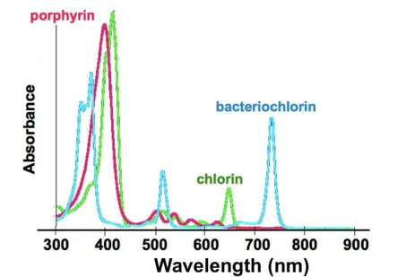
Among the endogenous and exogenous fluorophores emitting in the near-infrared region, porphyrins are suspected to be responsible for the near-infrared autofluores-cence. Many porphyrins are naturally occurring: one of the most famous is the heme, the pigment of red blood cells. The chlorines such as the chlorophylles can also be responsible for autofluorescence. In 1988, Weagle et al. observed that normal mouse skin had a fluorescence peak at 674 nm [35]. They attributed this fluorescence to a degradation product of chlorophyll derived from the mouse food (see spectra in Fig.I.11). By illuminating a mouse whole-body using a preoperative probe at 785 nm, Montcuquet observed an autofluorescent prevailing signal in the stomach and the intestines (see Fig. I.12 ).

Figure I.11 – Absorbance spectra of porphyrin and chlorine Adapted from http:

www.genopole.f r/IM G/pdf /BraultAtelierBiophotonique.

The autofluorescence in the near-infrared region can be due to the presence of porphyrin in the bloodstream and we have seen that the food can be fluorescent too. The hypothesis of porphyrins is possible but not consistent with the quantity of por-phyrins in the body. Porpor-phyrins remain the only described endogenous fluorophores that emit in the near-infrared region [26]. However, in order to avoid any autoflu-orescence signal Funovis et al. [36] fed their mice with chlorophyll-free food seven days before the near-infrared imaging. They still observed non identified autofluo-rescence signals in the near-infrared region. Finally, the autofluoautofluo-rescence sources in the near-infrared region are still not well-identified. Because we aim to track rare and individual cells we have to reduce spurious signals, such as autofluorescence in order to increase the signal-to-noise ratio.

I.3 Solution proposed to reduce the

autofluores-cence signal

In order to solve this problem, the fluorescence signal peak wavelength should lie in an absorption and diffusion free region and should be distinguishable, either spectrally or temporally, from the autofluorescence background. Therefore, we have to work with probes that absorb and emit in the near-infrared region. They must also have a high fluorescence quantum yield, be biocompatible and present a low

Figure I.12 – Whole-body autofluorescence signal of a normal mouse obtained using a preoperative probe with an excitation at 785 nm [37].

toxicity.

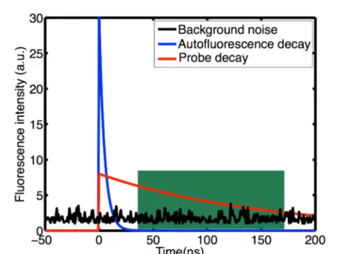
I.3.1 Time-gated detection coupled to long lifetime nanoprobes In the last few years, several groups have worked on time-gated detection in order to reduce autofluorescence for biological imaging. Fluorescence decay rate consists in isolating a time-decaying signal from other signals having a different (longer or shorter) timescale. In our case, autofluorescence has a short fluorescence lifetime so, time-gated detection using probes having longer fluorescence decay rates than autofluorescence would enable autofluorescence rejection and a substantial increase in the signal-to-noise ratio (principle in Fig. I.13). I will present the different techniques developed by several groups and describe one of the probes and imaging system chosen for each.

I.3.2 Current applications of time-gated detection for autofluo-rescence rejection

Confocal microscopy

Several groups have used time-gated detection in order to reduce autofluorescence signals. In 2001, Dahan et al. [38] built a stage-scanning confocal microscope with

Figure I.13 – Scheme of the principle of time-gated detection. In green adapted detection window.

a nanometer resolution closed-loop piezo-stage scanner. The excitation is provided by a Ti:sapphire laser, with an excitation at 503 nm and a 5 MHz repetition rate. At each piezo-stage step, the scanning controller generates a Transistor-Transistor Logic (TTL) pulse and a computer (which contains a time-correlated single-photon counting card) acquires the detected fluorescence photons. The start and stop pulses are provided by an avalanche photodiode and laser electronics, respectively (reverse mode). Thus, for each pixel of the image, they get histograms of photons arrivals. These histograms can be analysed in time-gated applications by selecting a time range of photons’ arrival and form an image with them. They incubated 3T3 mouse fibroblasts with a small amount of silanized visible quantum dots (λ = 575 nm, QY = 40%) overnight and fixed them. The QDs fluorescence decay could be described by a sum of three exponentials with characteristic times of 2, 8 and 24 ns that corresponds respectively to 11, 49 and 40 % of the fluorescence. Figure I.14 shows time-resolved confocal images. On top, the image corresponds to all detected photons. At the bottom, the image is obtained from photons that arrived between 35 and 65 ns after the laser pulse. The image was taken with a 25-ms integration time per pixel. The gated image allows the observation of bright, localized spots with enhanced signal-to-background ratio. Here, with the parameters used, they obtained a signal-to-noise

ratio of 15.

Figure I.14 – Time-resolved confocal image of a fibroblast previously incubated with quantum dots. a) Image obtained for all detected photons. b) Gated image built with photons that arrived between 35 and 65 ns after the laser pulse. [38]

This application of time-gated detection allows them to enhance the detection sensitivity by one order of magnitude. However, they used visible-emitting quantum dots, which are often made of cadmium (in this range of emission wavelength). In addition, excitation and emission wavelengths used here are not in the optical therapeutic window. Finally, with a 25-ms integration time per pixel, it requires several minutes to get an image. Such a time scale is not compatible with cell tracking measurements.

Whole-body imaging using near-infrared-emitting quantum dots

In 2009, May and co-workers [39] built a wide-field time-gated preclinical imaging system for detection of near-infrared-emitting quantum dots by suppression of the short-lifetime background autofluorescence. The near-infrared-emitting quantum

dots used here have a fluorescence lifetime superior to 20 ns. The imaging system consists in a pulsed high-power 630-nm LED excitation (2 MHz repetition rate) and a gated intensified CCD camera for fluorescence detection. The excitation light was bandpass filtered with filters at 615±20 nm to discriminate excitation light that overlapped with the quantum dot emission peak. The emission signal is similarly filtered using filters at 710 ± 25 nm to select fluorescence from quantum dots. The laser pulse and the intensifier are controlled by phase-locked generators and the in-tensifier is imaged on a CCD camera. In order to compare the efficiency of their time-gated detection compared to conventional fluorescence imaging, they synthe-sized images by overlapping the excitation pulse and intensifier detection window times during the image exposure (image called CW for continuous wave excitation). Alternatively, time-gated images were obtained by inserting a delay between the end of the excitation pulse and start of the detection gate. They injected a solution of QDs in Phosphate buffered saline (PBS) at different concentrations along the back of three anaesthetized nude mice and imaged the injection points. Figure I.15 shows images of the three mice previously injected with QDs in CW (on the left) and superposition of CW (in green) and the time-gated (in red) images on the right. Time-gated detection greatly improved contrast of QDs, allowing a detection of QD concentrations down to 0.25 nM. Depending on the concentration, the exposure time was variable, from 125 ms to 5 s. The delay is empirically fixed at 50 ns after the laser pulse. The image contrast, defined as the ratio between QDs signal and the autofluorescence, increased by a factor from 3 to 10 using time-gated detection.

This application of time-gated detection allows an enhancement of near-infrared quantum dots detection. Moreover, the quantum dots used have an emission wave-length in the optical therapeutic window. However, this type of quantum dots is composed of heavy metals (cadmium and tellurium). The imaging set up is a whole-body imaging system, which has not the spatial and temporal resolutions necessary for individual cell tracking.

Whole-body imaging using silicon nanoparticules

Recently, Gu et al. have imaged a human ovarian cancer xenograft in a mouse model using porous silicon nanoparticules introduced via intravenous injection [40]. Synthesized porous silicon nanoparticles have a mean hydrodynamic diameter of 168 nm. Their emission wavelength is centered at 800 nm (QY = 10%) and their fluorescence lifetime is 12 µs, about 1000 times longer than the autofluorescence. A

Figure I.15 – Wide-field images of 3 nude mice subcutaneously injected with near-infrared-emitting QDs at different concentrations along their backs. a) Image obtained with continuous wave (CW) illumintation. b) Superposition of CW images (in green) and time-gated images (in red) with a 50 ns delay after the laser impulsion [39].

time-domain fluorescence imaging system eXplore Optix is used to image mice in

vivo. The system was used with a 470-nm excitation laser with a repetition rate of

40 MHz, corresponding to a 25 ns time window between pulses. CW fluorescence images are obtained by reconstructing the photoluminescence signal collected us-ing the full 25 ns time-window from the data. For time-gated (TG) fluorescence images the photoluminescence signal was collected between 20.5 and 21.5 ns of the imaging time-window from the full data. Figure I.16 presents CW and TG images of a nude mouse bearing a human ovarian cancer xenograft at different time after injection of silicon nanoparticules. The white arrow indicates the tumour localiza-tion. Just after injection, no signal from nanoparticles is observed in the tumour location. One hour after injection, CW image does not indicate difference of con-trast between normal tissue and tumour tissue. However, time-gated image shows a weak photoluminescent signal at the tumour location. Four hours post-injection, the authors observe a different contrast between CW and TG images at the tumour location. Silicon nanoparticles have accumulated in the tumour location are their presence was clearly revealed using the TG detection. The signal at the tumour location decreases 24 hours post-injection, which suggests that a degradation and clearance from the host occur [41].

Figure I.16 – CW and time-gated images of nude mouse bearing a human ovarian carcinoma SKOV3 xenograft tumour at different time after the porous silicon nanoparticles injection [40].

Their fluorescence quantum yield is relatively high (10%) in this range of emission wavelengths. These nanoparticles are biodegradable, which ensures a low level of toxicity. Because we aim to track cells over a few days, they need to be massively charged with nanoprobes. Indeed, the cell division leads to a probes dilution between the two daughter cells. Here, the high hydrodynamic diameter of the nanoparticles limits the massive loading of cells with nanoprobes and decreases the number of days during which cells can be tracked. Moreover, this optical system by photons counting requires a long acquisition time and important analysis treatments in order to obtain the definitive image. In our application, because we want to determine the metastatic migration pathway we need to track dynamic cells. Finally, this system does not allow a cell-scale detection, and therefore a detection of isolated and rare cells.

Wide-field imaging and flow cytometric analysis

Nanodiamonds are promising fluorescent biomarkers because they are highly pho-tostable and biocompatible [42]. Very recently, Hui et al. [43] reported their use to detect cancer cells in blood analysis. Here, nanodiamonds have an emission

wave-length centered at 700 nm, their fluorescence lifetime is around 20 ns and their diameter is 100 nm.

The optical set up was a wide-field microscope with an excitation at 600 nm. The detection was performed by a nanosecond intensified charge-coupled device. Figure I.17 shows images of HeLa cells stained with nanodiamonds and immersed in human blood in order to mimic in vivo autofluorescence signal. The left image is a typical wide-field fluorescence image and the right image is a wide-field time-gated image. The exposure time used for fluorescence images is 0.1 s and for time-gated images 0.3 s. They use a 100X immersion oil objective. They clearly observed a sensitivity enhancement with the time-gated detection that was confirmed by the intensity profiles of both images.

Figure I.17 – In vitro images of HeLa cells stained with nanodiamonds and immersed in human blood. a) Wide-field fluorescence classical image. b) Time-gated image. c) Intensity profiles along the black and red color lines of images just above [43].

They also performed flow cytometry using their system. They used microchannel devices with dimension compatible to mouse and rate blood capillaries. The cell counting was performed using a MATLAB program that also allowed measuring

fluorescence intensity of nanodiamond-labelled cells. Finally, to demonstrate the principle that their wide-field imaging system may serve as a useful instrument for

in vivo flow cytometry they labelled mouse lung cancer cells with nanodiamonds

and then injected them into a mouse via its tail vein. Figure I.18 presents in vivo images of mouse blood vessel where a stained cell pass though.

Figure I.18 – In vivo images of mouse lung cancer cells stained with nanodia-monds and injected in a mouse bloodstream via the tail vein. [43].

The experiments use nanodiamonds that are biocompatible and easily taken up by cells for labelling. Their diameter is 100 nm and their fluorescence lifetime is 20 ns. The optical set up developed allows a cell-scale imaging with an enhance in sensitivity by autofluorescence rejection. However, the fluorescence lifetime of nan-odiamonds is not so far from the autofluorescence one. This limits a total rejection of the autofluorescence. To the best of our knowledge, this article is the first one that clearly shows images of isolated cells in an in vivo sample using time-gated detection.

I.4 Conclusion

This state of the art of the current imaging techniques for in vivo cell tracking al-lowed us to determine that fluorescence imaging is a sensitive technique that should permit the detection of isolated circulating cells. To overcome the two limitations in fluorescence imaging, we propose to stain cells with near-infrared long fluores-cence lifetime probes and to couple them to a time-gated detection to reduce the autofluorescence signal and improve the sensitivity. Several groups have worked on the development of time-gated imaging systems in order to reduce autofluorescence signals. The here-reported experiments utilize different types of nanoprobes with various fluorescence decays. Indeed, nanoprobes fluorescence decay has to be longer than the autofluorescence one.

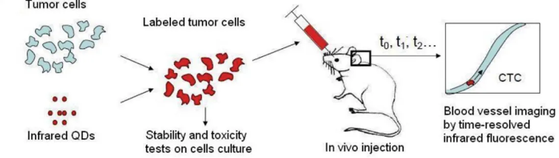
To conclude, optical microscopy seems to be the most adapted imaging tech-nique. In this manuscript, I will present our probe choice, their synthesis and opti-cal characterization. Then, I will describe the optiopti-cal set up we developed and the results obtained using both optical set up and nanoprobes. In order to determine the metastatic migration pathway, for the PIOL application, we plan to label cells with near-infrared-emitting long fluorescence lifetime probes. Toxicity test will be performed on these cells. Stained cells will be injected in the eye of a mouse model of PIOL, and we plan to observe them in the blood vessels of a mouse ear, as illustrated in Fig. I.19.

Figure I.19 – Scheme of the CTC detection principle using near-infrared-emitting nanoprobes coupled to time-gated detection (Scheme from Thomas Pons).

II

Near-infrared-emitting quantum dots for

cell labelling

II.1 Introduction

In order to efficiently detect in vivo circulating tumour cells, we have to be highly sensitive. Fluorescence microscopy is a technique that is very sensitive. Nevertheless, this sensitivity is limited by the low visible light penetration depth and the tissue autofluorescence. In order to reduce these two limitations, the fluorescent probes must have well-defined specifications. Indeed, we need probes with an emission wavelength in the "optical therapeutic window" and that present long fluorescence lifetime compared to the autofluorescence one. Nanoprobes also have to be small (to massively charge biological cells), biocompatible and present a low cytotoxic. Finally, as we aim to track cells over a few days, they need to keep their chemical and photo-stability in a biological environment.

There are several materials that have an emission in the near-infrared region [44]. We can remove from the list organic molecules that have fluorescence lifetimes too close from the autofluorescence. Among the existing materials, we selected different near-infrared emission and long fluorescence lifetimes nanoparticles : silicon nanoparticles, rare earth doped nanoparticles and quantum dots.

Silicon nanoparticles have the advantage of being non cytotoxic and biodegrad-able. Indeed, in 2009, Park et al. have reported that silicon nanoparticules self-destruct in a mouse model into renally cleared components in a relatively short period of time with no evidence of toxicity [41]. Their fluorescence lifetime is long (around 1-10 µs) but their fluorescence quantum yield is not enough high to detect rare and individual event (around 10 %). Rare earth also have excitation and emis-sion properties adapted for in vivo imaging. In 2013, Foucault-Collet et al. have synthesized near-infrared emitting lanthanides and have managed to obtain in vitro images of HeLa cells after probes incubation. Their fluorescence lifetime is long, however their diameter is high (a fraction of micrometer) and their fluorescence quantum yield is too low for our application of single cell tracking (a few percents) [45].

Quantum dots (QDs) are nanocrystals of semiconductors with an emission wave-length depending on their size and on their composition [46][47]. Their emission wavelength can be tuned from 300 nm to 5 µm. Because of their small size (around 5 to 10 nm), these nanocrystals present a different behaviour from the corresponding bulk semiconductor. QDs are composed of an inorganic core surrounded by an or-ganic outer layer of surfactant molecules (ligands) which aims to ensure the colloidal dispersion and to passivate the QD surface. The small size of these nanocrystals

implies great importance of surface effects that can degrade the fluorescence. An interesting strategy to improve nanocrystals surface passivation, and thus preserve a high quantum yield, is their overgrowth with a shell of a second semiconductor (typically ZnS) resulting in core/shell systems.

A nanocrystal can be considered as a nano-sized quantum box in which electrons are confined. The wave function associated with an electron in a nanocrystal is less spread compared to the bulk semiconductor. The electron is confined which costs energy and induces an increase of the band gap. This affects the electronic structure and tends to separate the electronic levels from each other, especially as the radius of the nanocrystal gets smaller: this effect is called quantum confinement. This leads to a red shift of the QD fluorescence as the size increases.

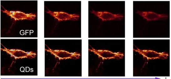
In the last few years, quantum dots have been used for biological applications [48][49] because they combine a high resistance to photobleaching and interesting optical properties. Figure II.1 shows a HeLa cell previously labelled with the Green Fluorescence Protein (GFP) on the top and with QDs on the bottom. The cell stained with QDs can be observed for a longer time compared to the GFP cell that photobleaches more rapidly.

Figure II.1 – Comparision of the photobleaching between a cell stained with GFP (on the top) and QDs (on the bottom). Images from Alexandra Fragola.

Many nanocrystals have a bandgap which yields an emission wavelength in the near-infrared region [50]: CdHgTe/ZnS [51], InAs [52] and CdTe [53]. However, the use of these kind of materials is limited because of the high toxicity of their heavy metals composition such as lead, cadmium or arsenic. Indium phosphide (InP) seems a good alternative as it can theorically reach emission wavelengths in

the optical therapeutic window. Unfortunately, the phosphorus precursors are rare and expensive [54], or release a deadly gas P H3 during the reaction [55]. Moreover,

it is difficult to provide InP nanocrystals big enough to reach near-infrared emission wavelength.

New types of quantum dots, commonly called I-III-VI (because of their chem-ical composition) have been synthesized [56][57][58]. They have the advantage of being composed of low toxic elements and their emission is tunable from green to near-infrared regions. CuInSe2 nanocrystals have a bandgap of 1.04 eV at 300 K

(corresponding to a theoretical maximum emission wavelength of 1.2 µm) and their Bohr radius is equal to 5.4 nm, which enables the confinement regime for smaller nanocrystals sizes. These materials have first been used for solar cells because of their low cost, abundance, optimal bandgap energy and their broad absorption spec-tra [59][60]. Then, they have been synthesized as colloidal nanocrystals via different methods : precursors decomposition [61][62][63], autoclave [64] or high temperature injection in organic medium [65]. Several groups have been interested in these ma-terials and have worked on their synthesis in order to improve their fluorescence quantum yield [65][66][67]. A solution to increase the fluorescence quantum yield was to add a shell, with a higher bandgap, around the core in order to confine the charges (electrons and holes) inside the cores [58][68]. This shell also allowed the preservation of the fluorescence properties after solubilization in water for in vivo biological fluorescence imaging [56][58][68][69][70].

Furthermore, most of the reported QDs syntheses are performed in organic sol-vent. Thus, QDs are surrounded by long organic strings as ligands and are not directly biocompatible. For this reason, we have to modify the quantum dots sur-face to provide biocompatible nanocrystals. It has been shown that QD sursur-face chemistry is not only responsible for the biocompatibility but also for the toxicity since it determines the biodistribution [71]. The ligand has to present different func-tions: one part which allows the QDs anchoring and another hydrophilic part which allows the water solubilization and biocompatibility. There are two main techniques [72] to water-solubilize nanoparticles: QDs encapsulation in amphiphilic polymers or phospholipid surfactants and ligand exchange [73][74].

This chapter will focus on the synthesis and characterization of nanocrystals and on their water solubilization before cell labelling. We will show that this type of quantum dots have adapted optical properties for in vivo time-gated and cell tracking imaging. We will then describe our chosen method in order to massively

label cells with near-infrared-emitting quantum dots (NIR QDs) previously made biocompatible using a ligand exchange.

II.2 Zn-Cu-In-Se cores

II.2.1 Synthesis

The core synthesis is inspired from the synthesis that Elsa Cassette et al. developed three years ago in our lab [58]. For this synthesis, all metal precursors (copper chlo-ride, indium chlochlo-ride, selenourea and zinc acetate) are mixed together in a three-neck flask in the presence of a solvent (octadecene) and some ligands (oleylamine, trioc-typhosphine and dodecanethiol). The solution is heated at 265◦C. Figure II.2 shows

a scheme of the set up used for quantum dots synthesis. The solvent commonly used for quantum dots synthesis is the octadecene (ODE) because its boiling point is sufficiently high (around 315◦C). Trioctylphosphine (TOP) behaves as a ligand.

Oleylamine (OLA) acts as a ligand and also activates the reaction with the selenium precursor. Dodecanethiol (DDT) has a high boiling point (280◦C) and stabilizes the

nanocrystals during the temperature increase. Figure II.3 presents the chemical for-mula of the different molecules used during the core synthesis. The nanocrystals are formed from 90◦C where the solution becomes yellow then red at 120◦C and brown

at 200◦C (see Fig II.4). The nucleation and growth of the nanocrystals occur as the

temperature increases. Figure II.5 shows the normalized photoluminescence spectra of Zn-Cu-In-Se cores with respect to the temperature. The more the temperature increases, the more the nanocrystals emit in the near-infrared region because of the quantum confinement. Heating is stopped immediately after the targeted emission wavelength is reached (about 820 nm) and the flask is quickly cooled down to room temperature to stop the reaction.

Cu-In-Se nanocrystals emission is due to defects or other trap states in the crystal structure. These defects are also responsible for the low fluorescence quantum yield and create deep-traps for the exciton. We noted that the incorporation of zinc during the core synthesis improves a lot the fluorescence quantum yield [75][76]. This may be attributed to defect passivation and filling of vacancy sites by Zn atoms inside the core. Figure II.6 shows the emission spectra divided by the absorbance at the excitation wavelength of CuInSe cores from Cassette et al. synthesis and Zn-Cu-In-Se cores I have developed. This figure shows that for the same emission wavelength Zn-Cu-In-Se cores are brighter up to 7 times than CuInSe cores without zinc.

Figure II.2 – Experimental set up for the QDs synthesis.

Figure II.3 – Chemical formula of the different ligands and solvents used for core synthesis.

Figure II.4 – Colloidal nanocrystals in hexane obtained at different temperatures under visible light (top) and UV lamp excitation (bottom).

Figure II.5 – Normalized photoluminescence (PL) intensity spectra of Zn-Cu-In-Se cores obtained at different temperatures.

Figure II.6 – Photoluminescence (PL) intensity spectra normalized by the ab-sorbance at the excitation wavelength of Zn-Cu-In-Se cores and CuInSe cores.

II.2.2 Structural properties

We have characterized the Zn-Cu-In-Se nanocrystals using several techniques:

• X-ray diffraction (XRD) informs us about the cristallographic structure and alloy composition,

• transmission electronic microscopy (TEM) allows us to determine the shape and to estimate the size distribution,

• energy dispersive X-ray spectrometry (EDX) is an analytical technique used for the elemental analysis or chemical element characterization of a sample.

X-ray diffraction (XRD)

This method uses an X-ray beam that interacts with the crystal. It causes the diffraction of the light beam in specific directions. The angles and the intensity of the diffracted rays are measured. By comparing the diffractogram obtained with reference crystal peaks, we determine the cristallographic structure of our crystal.

I-III-VI semiconductors generally have a chalcopyrite cristallographic structure as described in the scheme II.7(a). It corresponds to a quadratic structure. I-III-VI semiconductors can also exist in a cubic structure called zinc blende. Cations

(Copper, Indium and Zinc), represented as grey atoms in Scheme II.7(b), form a face-centered cubic lattice. Compared to the chalcopyrite structure, cations are located in the center of half tetraedric sites formed by the selenium atoms network (yellow atoms) and also form a face-centred cubic lattice. In this case, it forms a cubic structure because the cations are not ordered.

(a) (b)

Figure II.7 – Scheme of the different cristallographic structures for Cu-In-Se based nanocrystals. a) Quadratic structure. b) Cubic structure. Yellow atoms stand for selenium atoms, grey atoms, blue atoms and pink atoms stand for cations.

In order to determine the crystallographic structure of our cores we performed X-ray diffraction measurements. Figure II.8 presents a diffractogram of our cores in purple and the reference peaks of cubic CuInSe2 and ZnSe. Our core nanocrystals

diffractogram fits well with the CuInSe2 and ZnSe diffractograms in cubic structure

as shown in Fig. II.8 (cyan and orange peaks). We can now determine the percentage of each element in the alloy using Vegard’s law (see Appendix A). This law gives a relationship between the crystal lattice parameter of an alloy and the proportions of the constituent elements. If we assume that our QDs are an alloy of CuInSe2 and

ZnSe, we obtain as composition 56% of CuInSe2 and 44% of ZnSe in cubic structure.

Using these results we can determine the ratio between each elements, as show in Table II.1.

These data allow us to determine the cores composition and density and estimate the cores concentration (see Appendix A).

Figure II.8 – Diffractogram of Zn-Cu-In-Se core nanocrystals and reference peaks of cubic CuInSe2 and ZnSe nanocrystals (PDF 01-088-2345 (ZnSe) and PDF

Cu/Zn Cu/Se 1.27 0.36

Table II.1 – Ratios between the different elements that compose the cores obtained using the Vegard’s law.

We conclude that the cores are composed of an alloy of 56% of CuInSe2 and 44%

of ZnSe in cubic structure.

Transmission Electron Microscopy

Transmission electron microscopy (TEM) is a technique in which a beam of electrons is transmitted through a thin sample. The beam of electrons interacts with the sample as it passes through. An image is formed with the electrons transmitted through the sample.

We can determine the nanoparticle shape and size using transmission electron microscopy (TEM). Figure II.9 presents TEM images of the Zn-Cu-In-Se at different magnifications. The higher magnification allows us to visualize the crystalline planes of our cores. The cores have a diameter of 4.1±0.4 nm.

(a) (b)

EDX measurements

In EDX measurements, an incident electron beam excites a core electron of an atom, ejecting it and thus creating an electron hole where the electron was. An electron from an outer higher-energy orbital fills the hole, and the energy difference may be released in the form of an X-ray. The number and energy of the X-rays emitted from a transition can be measured by an energy-dispersive spectrometer. Since the X-rays energy is characteristic of the energy difference between the two electronic levels and of the electronic structure of the element. This allows us to determine the relative composition of the sample measured.

The different ratios between all elements present in the cores are presented in the table II.2.

Cu/In Cu/Zn Cu/Se Cu/S

1.10±0.05 1.020± 0.002 0.61± 0.03 0.470±0.003

Table II.2 – Ratios between the different elements that compose the cores

These results confirm the presence of zinc in high quantity in the cores. However, these results are slightly different from those obtained in XRD. The ratio Cu/S reports the presence of sulfur in our cores samples. The presence of sulfur may be attributed to the dodecanethiol as ligand or to the dodecanthiol that can be decomposed and incorporated in the core during the synthesis. However, if the amount of sulfur was higher, XRD peaks would have been shifted to the higher angles because ZnS or CuInS2 have a smaller lattice parameter (Bragg’s law). Therefore,

for the concentration calculation we will consider that the cores are only composed of CuInSe2 and ZnSe (see Appendix A).

This analysis confirms the presence of copper, indium, selenium and zinc in the cores, as observed in XRD. This also confirms a high incorporation of zinc in the core nanocrystals.

II.3 ZnS shell

In order to preserve the fluorescence and minimize the oxidation when a ligand exchange is performed, it was necessary to add a shell of another semiconductor material. The choice of the shell material depends on two main criteria. First, it has to have a larger bandgap in order to confine the charges (electron and hole)

inside the core. Second it has to have a lattice parameter close to the core’s one in order to allow the growth.

Zinc sulfide is a good candidate with a bandgap of 3.61 eV and a lattice parameter of 5.41 Å (5.78 Å for CuInSe2) [47]. Moreover, it is composed of non toxic elements

and has a good resistance towards oxidation allowing a better photostability. A final argument for the choice of a ZnS shell is the good affinity of the cationic atoms (Zn2+_{) with the dithiol function of the anchoring function of the}

poly(dithiol-co-sulfobetaine) ligand noted PDSB, used for water solubilization.

II.3.1 Synthesis

The precursors synthesis is described in the Protocols chapter and their formula are illustrated in Fig.II.10.

For the shell synthesis, 4 mL of as-prepared cores was dispersed in 4mL of ODE and 1mL OAm into a new three-neck flask. The mixture is degassed under vacuum at 40◦C. A solution of zinc ethylxanthate (Zn(EtX)

2) and zinc oleate (Zn(OA)2)

(0.13 and 0.8 mmol, respectively) dissolved in ODE (2 mL), TOP (3 mL), and dioctylamine (1 mL) is loaded into an injection syringe. The dioctylamine is added to facilitate the precursors dissolution in ODE.

The flask is heated to 190◦C under argon atmosphere and these ZnS precursors

are added dropwise during one hour. At the end of the injection, the reaction flask is cooled down to room temperature. The resulting Zn-Cu-In-Se/ZnS QDs are finally precipitated with ethanol and redispersed in 10 mL of hexane.

Figure II.10 – Chemical formulas of zinc and sulfur precursors used for the shell synthesis.