WASTE HEAT RECOVERY RANKINE CYCLE BASED SYSTEM
MODELING FOR HEAVY DUTY TRUCKS FUEL SAVING
ASSESSMENT
V. Grelet1,2,3, V. Lemort2*, M. Nadri3, P. Dufour3, T. Reiche1
1Volvo Trucks GTT ATR
1 av Henri Germain, 69800 Saint Priest [email protected], [email protected]
2Thermodynamics Laboratory – University of Liège,
Campus du Sart Tilman, B49, 4000 Liège, Belgium [email protected]
3Université de Lyon, F-69622, Lyon, France, Université Lyon 1, Villeurbanne, France CNRS,UMR
5007, LAGEP,
[email protected], [email protected] * Corresponding Author
ABSTRACT
This paper presents a method to model heat exchangers used in waste heat recovery Rankine based systems in heavy duty trucks. The method is developed to predict both transfer and working fluid physical properties such as temperature and density after the heat exchange process. Due to the flexibility of such a model, it can be used for a numerous quantity of fluids including water-alcohol mixture. A validation of the developed model is shown and compared to steady state and dynamic test results. The model shows good performance as well in terms of accuracy, which is in the range of 5K error as in computational time which is faster than real time and makes it suitable for concept optimization, control and fuel economy evaluation.
1. INTRODUCTION
Driven by future emissions legislations and increase in fuel prices, engine gas heat recovering has re-cently attracted a lot of interest. In the past few years, a high number of studies have shown the interest of energy recovery Rankine based systems for heavy duty (HD) trucks engine compounding [Espinosa (2011), Sprouse III and Depcik (2013)]. Recent studies have brought a significant potential for such a system in a long haul truck which can lead to a decrease in fuel consumption of about 5% and reduces en-gine emissions. But many challenges have to be faced before the vehicle integration. The correct choice of fluids and system architecture is approached in [Mago et al. (2007), Latz et al. (2012)] and shows that system simulation is a critical part of the development work. Moreover, several papers focused on the control strategy which is important in order to optimize the energy recovery process and maximize the power production as to ensure a safe operation of the system when talking from a system point of view. The high number of interactions, both with the engine and the vehicle, constrains the system and challenge the control design. The system dynamic is mainly controlled by the heat exchangers behavior (i.e. evaporators and condenser) and dynamic models of these components are of two kind: moving boundary (MB) [Zhang and Zhang (2006), Bendapudi et al. (2008)] and finite volume (FV) [Feru et al. (2013), Vaja (2009)]. Usually more complex in terms of computational capacity needed due to the high number of system states, the FV approach has the advantage to be more powerful and robust concerning the prediction. Both approaches have been widely used in large power recovery system and control sys-tem design [Horst et al. (2013), Peralez et al. (2013)] and results in a simplification of the heat recovery
Paper ID: 67, Page 2
boiler/condenser geometry in a great extent (i.e. by representing the boiler by a straight pipe in pipe counterflow heat exchanger). The use of water-alcohol mixture can bring some advantages in the power recuperation and overcome both disadvantages of these fluids: high freezing temperature of water and flammability of alcohol [Latz et al. (2012)]. In those blends, Water Ethanol is promising and compliant with vehicle integration where both pure fluids are not. In the following a FV model of evaporators recovering heat from EGR and Exhaust in a serial arrangement (EGR as preheater and exhaust as super-heater) using a mixture of 80% ethanol and 20% water by mass is presented and compared to steady state and dynamic tests. The paper is organized as follows. Section 2 presents the principle and the layout of the studied system. Section 3 presents the model itself and the resulting PDE system as well as the ODE discretized model. Section 4 compares modeling and experimental results when conclusions are drawn in section 5.
2. PRINCIPLE OF OPERATION AND STUDIED SYSTEM 2.1 Rankine process
The Rankine cycle is a widely used power generation cycle when it comes to turn heat into mechanical or electrical power. First, the working fluid is pumped from a tank at the condensing pressure to the evaporator at the evaporating pressure. Then the pressurized working fluid is pre-heated, vaporized and superheated in one or several heat exchangers. These heat exchangers are linked to the heat source. The superheated vapour expands from evaporating pressure to condensing pressure in an expansion device converting the pressure drop into mechanical work. Finally, the expanded vapour condenses through a condenser releasing heat into the cold sink (e.g. ambient air) and returns to the working fluid reservoir. In this process the changes of states in both the pump and the expander are irreversible and increase the fluid entropy to a certain extent. The process can be characterized as well by the Net Output Power (NOP) which corresponds to the generated power minus the pump consumption as well, as the cycle efficiency which is the ratio of the net output power by the heat flow rate recovered during the evaporation.
2.2 Studied system
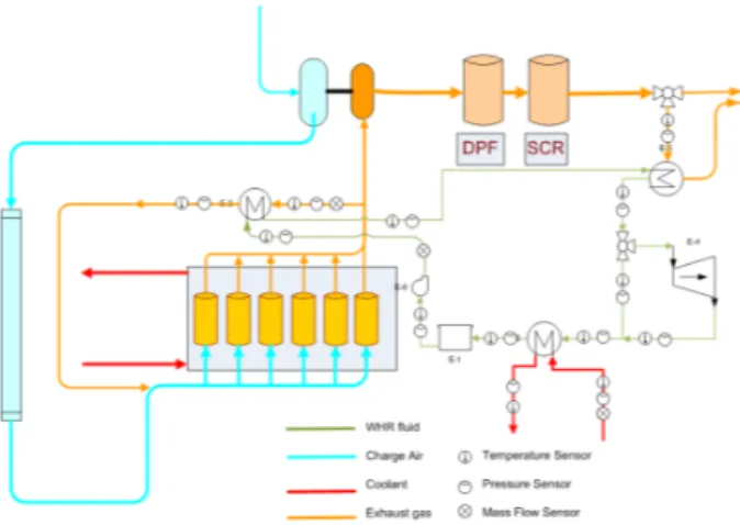
The waste heat recovery system (WHRS) is compounded on a turbocharged 6 cylinder 13L 320kW HD engine using exhaust gas recirculation (EGR) and selective catalist reduction (SCR) to reduce the NOx emissions. The studied Rankine cycle is recovering heat from both EGR and exhaust, but unlike [Teng (2010)], heat exchangers (HEX) are arranged in a serial configuration in order to ensure low temperature of the EGR gases at the intake manifold inlet. This layout is also advantageous concerning the number of valves and actuators needed and simplify the control since there is a single controlled mass flow rate. The chosen working fluid is composed of water (20% wt) and ethanol (80% wt). The mass flow rate through the two boilers is controlled by the pump speed. The expansion machine is a turbine which has a higher power density than volumetric expanders [Kunte and Seume (2013)]. The working fluid is then condensed through an indirect condenser fed by coolant. Moreover the cycle is equipped with two bypass valves: one located in the exhaust stream to control the amount of energy introduced in the system and a second in front of the expander to prevent liquid to enter in the turbine and avoid blade erosion caused by liquid droplets into a high speed rotor. The experimental setup is fitted with pressure, temperature and mass flow sensors on the working fluid and gases flow. Pressures and temperatures are measured before and after each component in order to characterize their performance. Mass flow sensors are installed downstream the pump for the working fluid (based on the coriolis effect) and upstream their respective boiler for EGR and exhaust gases (based on the venturi effect). The sensors uncertainties given by the manufacturers are in the range of +/- 3K for the working fluid thermocouple, +/- 1.5% for the gases thermocouple, +/- 3% for the piezoresistive pressure sensors and 0.5% for the mass flow rates. Furthermore sensors performance can be influenced by other parameters such as the temperature field distribution among the pipe area for temperature sensors and the flow pulsation for the working fluid mass flow sensor. The complete experimental setup is presented in Figure 1. Recorded data during the test campaign are hereafter used to calibrate and validate the models of the EGR and exhaust gas boiler.
Figure 1: Experimental Setup
3. HEAT EXCHANGER MODEL
The models are developed to dynamically predict temperature and enthalpy of primary and secondary fluid (also called in the following working and transfer fluid) at the outlet of each boiler. This is critical when coming to control design to ensure a safe operation of the system and a proper operation of the EGR function. Safe means that the fluid is fully vaporized when entering the turbine in order to not destroy it. For the EGR, the aim is to have a gas temperature exiting the boiler at least equal to the one when using a classical cooler to not to disturb the emissions control strategy and the combustion process.
3.1 Modeling assumptions
Several assumptions have been made in order to simplify the dynamic problem. These ones are generally accepted when it comes to dynamic modeling of heat exchangers with phase change [Vaja (2009)].
• The transfer fluid is always considered in single phase i.e. no condensation in the EGR/exhaust gases is taken into account.
• The conductive heat fluxes are neglected since the predominant phenomenon is the convection. • Pressure drop in each fluid (transfer and working fluids) is not considered.
• Both boilers are represented by a straight pipe in pipe counterflow heat exchanger, similarly to Vaja (2009), divided into n lumped sub-volumes in the longitudinal direction.
• Fluid properties are evaluated at the outlet of each sub-volume.
• Pressure dynamics is neglected since its time scale is very small considered to relevant HEX ones.
3.2 Governing equations
The model presented in this paper is based on mass (1) and energy conservation (2) equations.
Across ∂ ρj ∂t + ∂ ˙mj ∂z = 0, (1) Across ∂ ρjhj ∂t + ∂ ˙mjhj ∂z + ext ∑ i=int ˙ qjk = 0, (2)
where: ˙qjk = αjPEexchjk(Twallk− Tj) with : k = int, ext and j = f, g, amb.
On the working fluid side, both conservation principles are applied whereas on the transfer fluid side the variation in density due to temperature and pressure change is neglected: therefore the continuity equa-tion is not implemented in this region. These conservaequa-tion principles at each node can be applied:
Paper ID: 67, Page 4
• Fluid Side (inner pipe): As pressure dynamics is neglected, the derivative term in density becomes:
∂ ρf ∂t = ∂ ρf ∂hf ∂hf ∂t . (3)
By implementing equation (3) in (1) it takes the following form:
Across ∂ ρf ∂hf ∂hf ∂t + ∂ ˙mf ∂z = 0. (4)
The energy conservation principle is then described by:
Acrossf
∂ ρfhf
∂t + ∂ ˙mfhf
∂z + ˙qfint = 0. (5)
• Gas side (outer pipe): The density change due to temperature decrease in the heat exchangers is rather small (below a ratio of 2), therefore the continuity equation (1) is neglected and only the energy conservation principle (2) is applied where enthalpy is taking the following form:
hg= cpg(Tg)Tg. (6)
The energy conservation principle showed in equation (2) is then expressed under the following form:
∂ ˙mgcpg(Tg)Tg
∂z +
∂ ˙mgcpg(Tg)Tg
∂t + ˙qgint+ ˙qgext = 0. (7)
• Internal pipe wall: An energy balance is expressed at the wall between the two fluids and is written as follows:
˙qfint+ ˙qgint =
∂mwintcpwintTwint
∂t . (8)
• External pipe wall: Similarly to the internal wall the balance of the entering and leaving heat fluxes is done on the external wall:
˙qgext+ ˙qaext =
∂mwextcpwextTwext
∂t . (9)
In addition to those equations, boundary and initial conditions are needed at z = 0 and z = L. Time
dependent boundary conditions are used: ˙
mf(t, 0) = ˙mf0(t) ∣ ˙mg(t, L) = ˙mfL(t)
hf(t, 0) = hf0(t) ∣ Tg(t, L) = TgL(t)
(10) The initial conditions for each state is given by:
˙
mf(0, z) = ˙mfinit(z) ∣ Tg(0, z) = Tginit(z) ∣ Twint(0, z) = Twintinit(z)
hf(0, z) = hfinit(z) ∣ ∣ Twext(0, z) = Twextinit(z)
(11)
3.3 Heat transfer
To model the convection from the transfer fluid to the pipe walls and from the internal pipe to the work-ing fluid, a heat transfer coefficient (α) is needed. The convection from a boundary to a movwork-ing fluid is usually represented by the dimensionless Nusselt number (Nu), which is the ratio of convective to conductive heat transfer and is equal to:
Nu= αl
λ, (12)
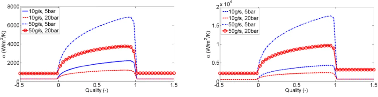
where l represents a characteristic length and is, here, the hydraulic diameter. Numerous correlations to approach this number (α) can be found in the literature [Thome (2010)] and are usually derived from
Figure 2: Heat transfer coefficient profiles EgrB (left) and ExhB (right)
experiments. Those correlations depend on the flow regime, the number of phases and the geometry studied. In single phase the following correlation is implemented:
Nu= CRenPrm, (13)
where C is a constant, Re and Pr are dimensionless number (respectively Reynolds and Prandtl number). By integrating those numbers expressions in equation (13), it becomes:
Nu= C ( 4 ˙m πdhμ) n (cpμ λ ) m . (14)
In the single phase region, the heat conductivity (λ), the viscosity (μ) and the specific heat (cp) are
assumed constant and the following expressions for the heat transfer coefficient is then derived:
αfliq = αfliqrefm˙fnfliq ∣ αfvap = αfvaprefm˙fnfvap ∣ αg = αgrefm˙gngas (15)
where the constant αrefand the exponent n have to be identified in liquid and vapor region for the working
fluid and in single phase for the gas. In two phase, a correlation similar to [Horst et al. (2013)] is used to enhance the single phase heat transfer coefficient. This correlation corresponds to a tube arrangement and is practical since it creates continuity between single and two phase heat transfer coefficient and does not need transport properties such as viscosity or heat conductivity.
αf2φ= αfliq ⎧⎪⎪⎪ ⎨⎪⎪ ⎪⎩(1 − x) 0.01⎡⎢⎢⎢ ⎢⎣(1 − x) + 1.2x 0.4(ρliq ρvap) 0.37⎤⎥ ⎥⎥ ⎥⎦ −2.2 + x0.01⎡⎢⎢⎢ ⎢⎣ αliq αvap ⎛ ⎝1+ 8 (1 − x) 0.7(ρliq ρvap) 0.67⎞ ⎠ ⎤⎥ ⎥⎥ ⎥⎦ −2⎫⎪⎪⎪ ⎬⎪⎪ ⎪⎭ −0.5 , (16) where x is the fluid quality defined as the quantity of vapor presents in the two phase flow:
x= ⎧⎪⎪⎪ ⎪⎪ ⎨⎪⎪ ⎪⎪⎪⎩ 0 if hf≤ hsatliq hf−hsatliq
hsatvap−hsatliq if hsatliq ≥ hf≤ hsatvap
1 if hf≥ hsatvap
(17)
Figure 2 show the working fluid heat transfer coefficient (α) for the EGR (left) and exhaust (right) boilers.
For convenience, the quality (x) is not bounded between the interval[0, 1] as shown in equation 17.
3.4 Working fluid properties
The working fluid properties are approximated using mathematical descriptions. This allows being in-dependent from thermochemical database such as [Eric. W. Lemmon (2013)] and creates continuity in derivative terms during the single / two phase transition. The fluid properties will only be functions of pressure and enthalpy.
Paper ID: 67, Page 6 • Temperature model: Tf= ⎧⎪⎪⎪ ⎪⎨ ⎪⎪⎪⎪ ⎩
aTliqh2f + bTliqhf+ cTliq if hf≤ hsatliq
Tsatliq+ x (Tsatvap− Tsatliq) if hsatliq ≥ hf ≤ hsatvap
aTvaph2f + bTvaphf+ cTvap if hf≥ hsatvap
(18)
where a., b. and c.are first order polynomial expressions function of pressure. The saturation
temperature (Tsat) is approximated with the Wagner equation with adapted coefficient for liquid
and vapor saturation [Kleiber et al. (2010)] and allows to make the transition between each phase. • Density model:
ρf=⎧⎪⎪⎪⎪⎨
⎪⎪⎪⎪ ⎩
aρliqh2f + bρliqhf+ cρliq if hf≤ hsatliq
1
aρ2φhf+bρ2φ if hsatliq ≥ hf≤ hsatvap
aρvaph2f + bρvaphf+ cρvap if hf≥ hsatvap
(19)
In single phase (liq and vap) the coefficient a., b.and c.are evaluated thanks to third order
poly-nomial function of pressure similar to:
aρ2φ = 1 aρ2φ 1Pf+aρ2φ0 ∣ bρ2φ= 1 bρ2φ 1Pf+bρ2φ0 (20)
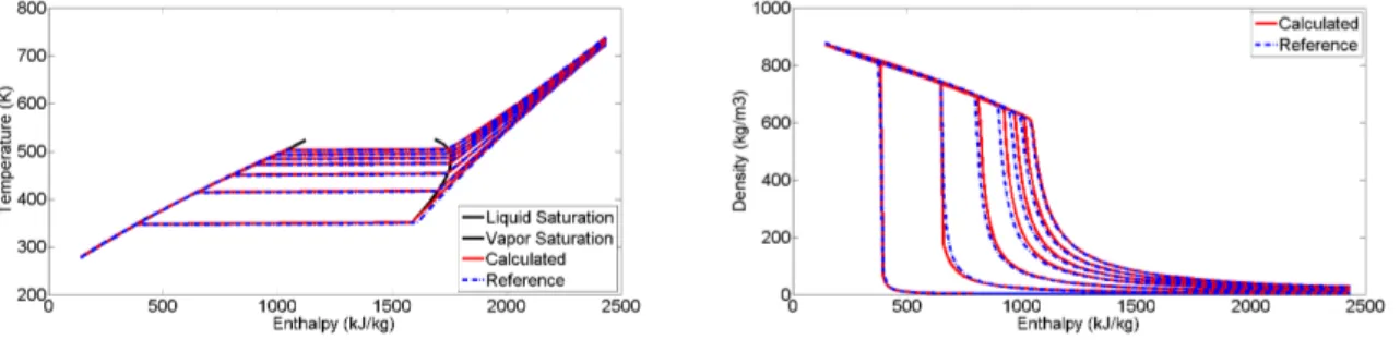
All coefficients mentioned before are evaluated thanks to fitting routines written in Matlab. Figure 3 show comparison between calculated temperature and density thanks to equation (18) and (19) and properties coming from [Eric. W. Lemmon (2013)] for pressure going from 1 to 80 bar.
Figure 3: Temperature (left) and density (right) model validation
3.5 Discretization
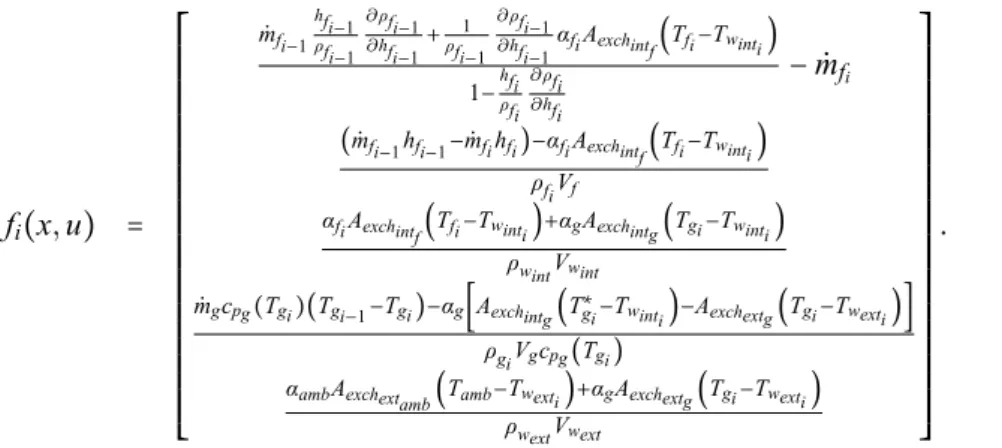
To be implemented in the simulation environment, the continuous model mentioned by equations (4), (5), (7), (8), (9) are discretized with respect to space, based on finite differences method: The heat exchanger is divided into n longitudinal cells where a backward Euler scheme is applied for the space derivative terms. The dynamic response of the ith cell can be described by:
u= [ ˙mf0 Pf0 hf0 m˙gL TgL] Z= ⎡⎢ ⎢⎢ ⎢⎢ ⎢⎢ ⎢⎢ ⎣ 0 0 0 0 0 0 1 0 0 0 0 0 1 0 0 0 0 0 1 0 0 0 0 0 1 ⎤⎥ ⎥⎥ ⎥⎥ ⎥⎥ ⎥⎥ ⎦ xi = [ ˙mfi hfi Twinti Tgi Twexti] Z˙xi= fi(xi, u) (21)
fi(x, u) = ⎡⎢ ⎢⎢ ⎢⎢ ⎢⎢ ⎢⎢ ⎢⎢ ⎢⎢ ⎢⎢ ⎢⎢ ⎢⎢ ⎢⎢ ⎢⎢ ⎣ ˙ mfi−1hfi−1 ρfi−1 ∂ ρfi−1 ∂hfi−1+ 1 ρfi−1 ∂ ρfi−1 ∂hfi−1αfiAexchintf(Tfi−Twinti) 1−hfi ρfi ∂ ρfi ∂hfi − ˙mfi
( ˙mfi−1hfi−1− ˙mfihfi)−αfiAexchint
f(Tfi−Twinti) ρfiVf
αfiAexchint
f(Tfi−Twinti)+αgAexchintg(Tgi−Twinti) ρwintVwint
˙
mgcpg(Tgi)(Tgi−1−Tgi)−αg[Aexchintg(T∗gi−Twinti)−Aexchextg(Tgi−Twexti)] ρgiVgcpg(Tgi)
αambAexchext
amb(Tamb−Twexti)+αgAexchextg(Tgi−Twexti) ρwextVwext ⎤⎥ ⎥⎥ ⎥⎥ ⎥⎥ ⎥⎥ ⎥⎥ ⎥⎥ ⎥⎥ ⎥⎥ ⎥⎥ ⎥⎥ ⎥⎥ ⎦ . (22)
where the ambient temperature Tambis assumed constant around the entire HEX.
4. HEX MODEL VALIDATION 4.1 Parameters identification
In the model presented above there are two kinds of parameters to identify. First: geometric parameters such as heat exchange area or cross section are usually given by the manufacturer or can directly be measured on the heat exchanger. Secondly: there are non-measurable parameters such as exponent in heat transfer correlation for each fluid. The identification process results into minimizing the error for each boiler on the working and transfer fluid outlet enthalpy or temperature using a feasible set of non-measurable parameters.
4.2 Steady state validation
First, the model is validated using steady state experimental results. To be representative of the engine map, 24 operating points corresponding to a speed/torque couple are used to compare experimental data to simulation results.
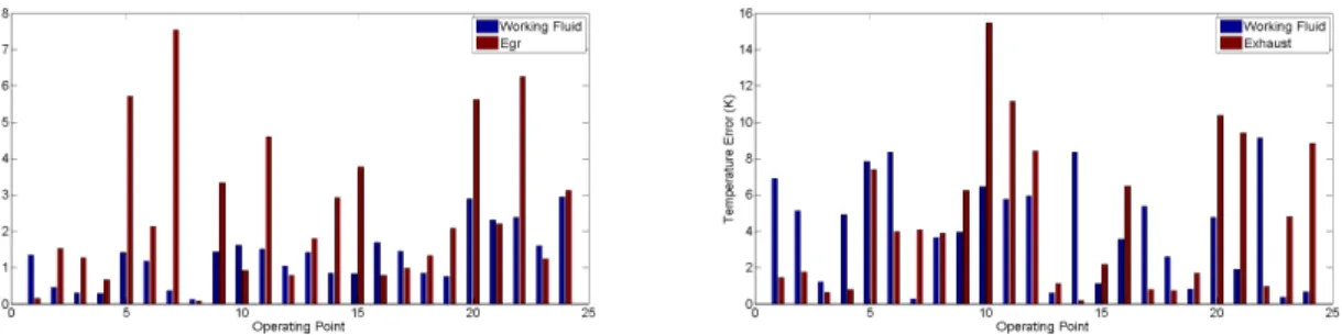
EGR evaporator: The comparison is done only for the EGR outlet temperature since in all
measure-ments the working fluid is in two phase state. During the phase change, the temperature is more or less constant (a small temperature increase is observed for mixture) and comparison is not relevant on this criterion (major source of error coming from the pressure which is considered constant in both boilers). Figure 4 presents the temperature difference observed on both fluids: transfer (EGR) and working fluid (water ethanol mixture). The maximum deviation observed on the EGR temperature is 7.6 K and the average error is around 2.6K.
Exhaust evaporator: Figure 4 presents the temperature difference observed between the model and the
experiments. Here both temperatures are relevant for comparison since the fluid is fully vaporized at the outlet. On the water ethanol side the maximum error is 9.2K and the mean deviation is around 4K. On the gas side the maximum error observed is 15.5K and the average difference is about 4.7K. Largest differences are observed on the exhaust which is not so important since accuracy on the working fluid is more significant for control purpose. The model predicts well the heat exchangers performance in steady state over the engine map. Main differences come from the non-dependency of the gas specific heat on air-fuel ratio (i.e. gases composition) and the uniform distribution of heat since the heat exchangers are simply represented by a single pipe. In reality, they are made of several channels and the working fluid is not necessarily homogeneously distributed between all the channels (this is also true for the gas). Last but not least, the heat losses are here represented by a single coefficient but in reality they are influenced by several parameters (external temperature and conditions). Moreover, one big issue was to have repetitiveness in the experiment. Indeed, the working fluid enters in the exhaust boiler in two phase state and it is assumed that the fluid distribution between each passage which was not homogeneous
Paper ID: 67, Page 8
creates those issues. In top of that, the different control loop actions (engine, Rankine and test cell) could have an influence on the experiments repetitiveness.
Figure 4: Temperature estimation error for the EGR (left) and Exhaust Boiler (right)
Steady state validation summary: Table 1 summarizes the model prediction error in steady state (relative
error is the ratio of the absolute error and the maximum temperature difference across the heat exchanger).
TfoutEgrB TfoutExhB TegroutEgrB TexhoutExhB
max mean max mean max mean max mean
Absolute (K) 2.95 1.30 9.15 4.16 7.54 2.54 15.47 4.71
Relative (%) 0.57 0.29 8.84 3.28 2.34 0.61 8.61 3.40
Table 1: Evaporators steady state validation
4.3 Dynamic validation
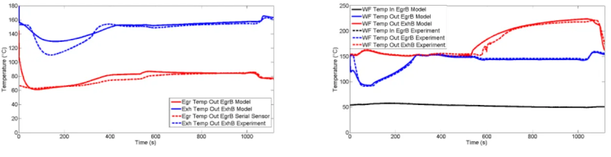
The model is then compared to dynamic experiments where either working fluid mass flow or EGR and exhaust conditions can vary. Figure 5 presents the experimental inputs used in the model. Figure 6 shows
Figure 5: Experimental inputs: gas (left) and WF side (right)
the model predicted temperature versus the measured ones for respectively gas and working fluid sides. A large error can be observed a time 0 due to the initial conditions. It was difficult to have access to certain values in the experimental setup to correctly set initial conditions in the model (e.g. internal and external wall temperatures). Nevertheless, the dynamic behavior of the complete system is relatively well represented with a maximum deviation of 26 K on the working fluid predicted temperature and 20 K on the gas side. The EGR boiler behavior is better represented due to the more simple geometry. Indeed this component has only one core and the simple representation chosen is pretty correct whereas the exhaust boiler is composed of two cores but as the split between each core was not known it has been decided to represent it as a single core heat exchanger.
Figure 6: Experimental and modeled temperatures
Dynamic validation summary: Table 2 presents a summary of the predicted errors in dynamic, for
sev-eral changes in the input disturbances. Even in dynamic, the model shows good ovsev-erall performance with mean deviations below 2.5% while the computationnal complexity is low.
TfoutEgrB TfoutExhB TegroutEgrB TexhoutExhB
max mean max mean max mean max mean
Absolute (K) 4.5 1.5 25.9 2.3 7.9 2.8 20 4.2
Relative (%) 1.38 0.46 14.37 1.28 2.43 0.86 11.1 2.33
Table 2: Evaporators dynamic validation
5. CONCLUSION
A dynamic model of a serial boiler arrangement Rankine cycle using water ethanol mixture and recover-ing heat from EGR and Exhaust is presented and compared to experimental results. The model presents the advantage to be low in terms of computational needs and is suitable for control software integration. A more complete transient validation is needed to fully validate the model but first results show pretty good accuracy both in steady state and dynamic with an average error lower than 2.5% (relatively to the maximum temperature difference across the heat exchanger). Future work will focus on high level con-trol strategy and optimization of the power recovery process on a complete vehicle environment. Low level control strategy is discussed in the companion paper [Grelet et al. (2015)].
REFERENCES
Bendapudi, S., Braun, J. E., and Groll, E. A. (2008). A comparison of moving-boundary and finite-volume for-mulations for transients in centrifugal chillers. International Journal of Refrigeration, 31(8):1437 – 1452. Eric. W. Lemmon, M. L. H. (2013). Refprop nist standard reference database 23 (version 9.0)), thermophysical
properties division, national institute of standards and technology, boulder, co.
Espinosa, N. (2011). Contribution to the Study of Waste Heat Recovery Systems on Commercial Truck Diesel
Engines. PhD thesis, University of Liege.
Feru, E., Kupper, F., Rojer, C., Seykens, X., Scappin, F., Willems, F., Smits, J., Jager, B. D., and Steinbuch, M. (2013). Experimental validation of a dynamic waste heat recovery system model for control purposes. In SAE
Technical Paper. SAE International.
Grelet, V., Dufour, P., Nadri, M., Lemort, V., and Reiche, T. (2015). Model based control for waste heat recovery rankine cycle system in heavy duty trucks. In 3rd International Seminar on ORC Power Systems (ORC15),
2015 (Accepted).
Horst, T. A., Rottengruber, H.-S., Seifert, M., and Ringler, J. (2013). Dynamic heat exchanger model for per-formance prediction and control system design of automotive waste heat recovery systems. Applied Energy, 105(0):293 – 303.
Paper ID: 67, Page 10
Kleiber, M., Wagner, W., Preisegger, E., Pfennig, A., and Neubronner, M. (2010). VDI Heat Atlas Second Edition,
Part D Thermophysical properties. VDI Buch. Springer.
Kunte, H. and Seume, J. (2013). Partial admission impulse turbine for automotive orc application. In SAE Technical
Paper. SAE International.
Latz, G., Andersson, S., and Munch, K. (2012). Comparison of working fluids in both subcritical and super-critical rankine cycles for waste-heat recovery systems in heavy-duty vehicles. In SAE Technical Paper. SAE International.
Mago, P. J., Chamra, L. M., and Somayaji, C. (2007). Performance analysis of different working fluids for use in organic rankine cycles. Proceedings of the Institution of Mechanical Engineers, Part A: Journal of Power and
Energy, 221(3):255–263.
Peralez, J., Tona, P., Lepreux, O., Sciarretta, A., Voise, L., Dufour, P., and Nadri, M. (2013). Improving the control performance of an organic rankine cycle system for waste heat recovery from a heavy-duty diesel engine using a model-based approach. In 52nd Annual IEEE Conference on Decision and Control (CDC), pages 6830–6836. Sprouse III, C. and Depcik, C. (2013). Review of organic rankine cycles for internal combustion engine exhaust
waste heat recovery. Applied Thermal Engineering, 51(1–2):711 – 722.
Teng, H. (2010). Waste heat recovery concept to reduce fuel consumption and heat rejection from a diesel engine.
SAE International Journal of Commercial Vehicle., 3:60–68.
Thome, J. R. (2010). Wolverine Tube Inc Engineering Data Book III. Heat Transfer Databook. Wolverine Tube Inc.
Vaja, I. (2009). Definition of an object oriented library for the dynamic simulation of advanced energy systems:
Methodologies, Tools and Applications to Combined ICE-ORC Power Plants. PhD thesis, University of Parma.
Zhang, W.-J. and Zhang, C.-L. (2006). A generalized moving-boundary model for transient simulation of dry-expansion evaporators under larger disturbances. International Journal of Refrigeration, 29(7):1119 – 1127.
NOMENCLATURE
Acronyms
EGR Exhaust gas recirculation
HD Heavy duty
HEX Heat exchanger
NOP Net output power
WHRS Waste heat recovery system Greek letters
α Heat transfer coefficient (W/m2/K) η Efficiency (−) λ Heat conductivity (W/m/K) ρ Density (kg/m3) Latin letters ˙ m Mass flow (kg/s) ˙
Q Heat flow rate (W)
˙q Linear heat flow rate (W/m)
A Area (m2) cp Specific heat (J/kg/K) h Enthalpy (J/kg) Nu Nusselt number (−) P Pressure (Pa) PE Perimeter (m) Pr Prandtl number (−) Re Reynolds number (−) T Temperature (K) t Time (s) V Volume (m3) z Spatial direction (m) Subscripts amb Ambient conv Convection
cross Cross section
egr EGR gas
EgrB EGR boiler
exh Exhaust gas
ExhB Exhaust boiler
ext External wall
f Working fluid
g Gas
in Inlet port
int Internal wall
liq Liquid
out Outlet port
sat Saturation
vap Vapor