An optical Solution for Simultaneous in-situ Sea Water Salinity and Turbidity Measurements

(1)

HAL Id: tel-00719584

https://tel.archives-ouvertes.fr/tel-00719584

Submitted on 20 Jul 2012

HAL is a multi-disciplinary open access

archive for the deposit and dissemination of sci-entific research documents, whether they are pub-lished or not. The documents may come from teaching and research institutions in France or abroad, or from public or private research centers.

L’archive ouverte pluridisciplinaire HAL, est destinée au dépôt et à la diffusion de documents scientifiques de niveau recherche, publiés ou non, émanant des établissements d’enseignement et de recherche français ou étrangers, des laboratoires publics ou privés.

Salinity and Turbidity Measurements

Bo Hou

To cite this version:

Bo Hou. An optical Solution for Simultaneous in-situ Sea Water Salinity and Turbidity Measurements. Optics [physics.optics]. Télécom Bretagne, Université de Bretagne-Sud, 2012. English. �tel-00719584�

(2)

Sous le sceau de l’Université européenne de Bretagne

Télécom Bretagne

En habilitation conjointe avec l’Université de Bretagne-Sud

Ecole Doctorale - sicma

An optical solution for simultaneous in-situ sea water salinity

and turbidity measurements

Une solution optique pour la mesure simultanée in-situ de la

salinité et la turbidité de l’eau de mer

Thèse de Doctorat

Mention : STIC

Présentée par Bo Hou Département : OPTIQUE

Directeur de thèse : Jean-Louis de Bougrenet de La Tocnaye Soutenance le 11 janvier 2012

Jury :

M. Patrick Juncar, Professeur, CNAM (Rapporteur) M. Marc Le Menn, Docteur, SHOM (Rapporteur)

M. Jean-Louis de Bougrenet de la Tocnaye, Professeur, Télécom Bretagne (Directeur de thèse) M. Marc Sevaux, Professeur, UBS (Examinateur)

M. Philippe Grosso, Enseignant chercheur, Télécom Bretagne (Invité) M. Patrice Brault, Ingénieur de recherche, NKE (Invité)

(3)

(4)

Acknowledgements

First of all, I would like to thank Mr. Jean-Louis De Bougrenet De La Tocnaye, the director of my thesis, for kindly accepting me as his PhD student and for his precious help, understanding and trust during the three years of work. I am very grateful to him for leading me to the right direction of the research works, for his valuable advice, and for his help in reading and correcting my articles and his pertinent remarks.

I am very thankful to Mr. Philippe Grosso, my supervisor, for his great help in the three years of work. Mr Philippe Grosso helped me with much advice and numerous ideas, and taught me a lot of concepts and helped me to resolve many problems and questions. I would never forget the days of the interesting discussions and the days of working together in the laboratory.

I am particularly grateful to Mr. Zong Yan Wu, my supervisor. Without him, I could not have the chance to start my study in France and in TELECOM Bretagne. He helped me not only in work but also in my daily life. His advice and idea inspired me to find the right way at the beginning of my PhD study. His help and support last even after his retirement. I would always remember his kindness, precious help and support.

I gratefully acknowledge Mr. Damien Malardé for his great work in the first version of the refractometer, which inspired me to continue my work. Mr. Damien Malardé helped me to get familiar with the project and everything about the school, gave me a lot of advice and help of working in the laboratory. I will always remember his kindness, for which he was always such a pleasant co-worker.

I would like to thank the project NOSS (NkeElectronics Optical Salinity Sensor) for the financial support of my thesis.

I would like to express my deep gratitude to Mr. Patrick Juncar, director of Institut de Métrologie au Centre National des Arts et Métiers and Mr. Marc Le Menn, director of Laboratoire de Métrologie of Service Hydrographique et Océanographique de la Marine, who kindly agreed to be the reviewers of this work.

My sincere appreciation to Mr. Marc Servaux of Université de Bretagne Sud, Mr. Patrice Brault of NKE electronics, Mr. Laurent Delauney of Ifremer, Mr. Philippe Grosso of TELECOM Bretagne, and Mr. Jean Louis De Bougrenet De La Tocnaye, who kindly agreed to be the members of the defence jury of my thesis.

I would also like to thank all the members of NKE electronics, SHOM and Ifremer, for their contributions to my work of thesis, especially Mr. Patrice Brault and Mr. Olivier Guillerme of NKE, Mr. Marc Le Menn of SHOM, Mr. Laurent Delauny and Mr. Christian Podeur of Ifremer.

(5)

I am grateful to the administrative team and technical team of TELECOM Bretagne. More precisely, I would like to express my deep gratitude to Ms. Anne-Catherine Cariou and Ms. Jennifer Romer for their effective management of the administrative affaires associated with their great kindness and precious help, to Mr. Jean-Pierre Clère for his fantastic work of the mechanics, and to Ms. Aimée Johansen for her precious help in correcting my english writing.

I would like to thank my parents for their endless care and support during my three years of life overseas. Their understanding, encouragement and support helped me through many difficult times.

Finally, I would like to express my thanks to all the professors, students and colleagues at TELECOM Bretagne, for their kindness and support during my stay in Brest.

Brest, February 2012

(6)

Abstract

Salinity and turbidity are two important seawater properties for the physical oceanog-raphy. The study of physical oceanography requires a compact high-resolution in-situ salino-turbidi-meter. The main objective of this work is to propose, design and implement an optical solution to simultaneously measure the seawater salinity and turbidity. Our first study is carried out to design a high-resolution refractometer based on a laser beam deviation measurement by a Position Sensitive Device (PSD). The refractive index mea-surements obtained by the voltage value delivered by PSD have been evaluated to quantify the performances of the sensor. According to the obtained results, it is clear that this PSD-based refractometer is attractive for innovative applications in metrology. However, PSD lacks the capability to retrieve the power distribution information of laser beam, which is related to the turbidity measurements. On the contrary, Charge-Coupled Device (CCD) gives much more information of laser beam than PSD. In the second part of the thesis, a performance comparison between PSD and CCD combined with a centroid algorithm are discussed with special attention paid to the CCD-based refractometer. According to the operating principle of CCD-based system, five factors of CCD-based system: image window size, number of processed images, threshold, binning and saturation are evaluated to optimize the CCD-based refractometer. By applying the optimized parameters, the performance of CCD-based refractometer is better than PSD-based refractometer in mea-suring the refractive index. Furthermore, by applying different post-processing algorithms, CCD-based system possesses the capability of measuring the power distribution sensitive quantities. To show this advantage of CCD-based system, the attenuation measurement method is used to measure turbidity without modifying the refractometer configuration. The turbidity measurement and salinity measurements influence each other in a refrac-tometer. To overcome these influences, a CCD combined with a new location algorithm is used to measure both the refractive index and the attenuation. Several simulations and experiments are carried out to evaluate this new method. According to the results, the way to improve the resolution is discussed as well. Comparing to the nephelometer specified by the NTU standard, our method has been proved as a valid method to measure turbidity. By studying the performances of CCD-based refracto-turbidi-meter, 3 new prototypes are proposed to improve the salinity and turbidity measurement performance at the end of this thesis. They are expected to be applied in the current researches of physical oceanography.

Keywords: salinity, turbidity, refractometer, turbidimeter, position sensitive device, charge-coupled device, seawater, refractive index, attenuation, scattering

(7)

(8)

Résumé court

La salinité et la turbidité sont deux propriétés importantes pour comprendre le comporte-ment physique des océans. L’étude de l’océanographie physique a besoin d’un salino-turbidi-mètre in-situ, haute résolution. L’objectif de ce travail de recherche est de proposer, concevoir et réaliser de nouvelles solutions optiques dédiées aux mesures simultanées de salinité et de turbidité de l’eau de mer. Une première étude est menée, afin de démontrer la conception d’un réfractomètre à haute résolution basé sur une mesure de la déviation d’un faisceau laser par un dispositif de détection de position (PSD). La mise en place d’une plateforme de caractérisation des mesures d’indice de réfraction à l’aide d’une lecture de tension délivrée par le capteur de position a permis de quantifier les performances du cap-teur en terme de sensibilité. Au vu des résultats obtenus, il apparaît que ce réfractomètre basé sur la mesure de position du faisceau réfracté se présente comme particulièrement avantageux pour des applications en métrologie comme la salinité. Cependant, le PSD n’a pas la capacité de récupérer les informations de la distribution de puissance du faisceau laser, qui est liée à la mesure de la turbidité. Par contre, le dispositif à transfert de charge (CCD) donne beaucoup plus d’informations sur la distribution de la puissance du faisceau laser. Dans la deuxième partie de la thèse, une comparaison des performances entre le système avec PSD et le système avec CCD combiné à un algorithme de calcul du centre de gravité est discuté avec une attention particulière pour le réfractomètre avec CCD. Selon le principe du système basé sur CCD, cinq paramètres du système avec CCD: la taille de la fenêtre d’image, le nombre d’images traitées, le seuil, le «binning» et la saturation sont évalués afin d’optimiser le réfractomètre équipé d’un CCD. En appliquant les paramètres optimisés, les performances du système avec CCD sont meilleures que les performances du système avec PSD pour mesurer l’indice de réfraction. Par ailleurs, en appliquant les différents algorithmes de post-traitements, le système avec CCD possède la capacité de mesurer les propriétés, qui sont sensibles à la distribution de puissance. Pour montrer cet avantage du système avec CCD, une méthode basée sur la mesure d’atténuation de la lumière est utilisée pour mesurer la turbidité sans modifier la configuration du réfrac-tomètre. Cependant, les mesures de salinité et turbidité s’influencent mutuellement dans un réfractomètre. Pour surmonter ces influences, un CCD combiné à un nouvel algorithme est utilisé pour mesurer l’indice de réfraction et l’atténuation. Plusieurs simulations et expérimentations sont menées pour évaluer cette nouvelle méthode. Selon les résultats, la façon d’améliorer la résolution est aussi discutée. La validation de notre méthode est montrée par la comparaison de nos résultats avec ceux du néphélomètre spécifié par la standard NTU. En étudiant les performances du réfracto-turbidi-mètre basé sur CCD, 3 nouveaux prototypes sont proposés pour améliorer les performances des mesures de salinité et de turbidité à la fin de cette thèse.

Mots clés: salinité, turbidité, réfractomètre, turbidimètre, PSD, CCD, eau de mer, indice de réfraction, atténuation, diffusion

(9)

(10)

Résumé

Introduction

L’océanographie est une science qui étudie et décrit les océans de la Terre. Cette dis-cipline a la particularité d’être à cheval sur plusieurs domaines. On distingue en effet l’océanographie physique, biologique, chimique et géologique, mais on retrouve souvent des interactions très fortes entre ces différents domaines. Nous distinguons principalement l’océanographie physique, qui est l’étude des mouvements dans les océans, à toutes les échelles, des courants océaniques, jusqu’aux vagues en passant par les courants côtiers et les courants de marée. La méthode qu’elle utilise pour l’étude de ces phénomènes est d’étudier les propriétés physiques de l’eau de mer et leur distribution, par exemple, dans les zones côtière, offshore, et hauturière. Parmi ces propriétés physiques, la salinité, la température, et la pression sont les propriétés fondamentales. Une autre propriété très important pour les recherches océaniques dans la zone côtière est la turbidité, elle est liée à des particules en suspension. L’étude de l’océan réclame un capteur in-situ en haute résolution pour mesurer simultanément la salinité et la turbidité.

La salinité

Si intuitivement, la salinité représente le contenu en sels dissous dans l’eau de mer, il faut se rendre à l’évidence qu’il est impossible de la mesurer précisément, de manière simple et globale. La première définition précise de la salinité de l’eau de mer date de 1902 et elle se définit comme la masse totale des substances solides dissoutes (en grammes) contenu dans un kilogramme d’eau de mer.

Cette définition est celle de la salinité absolueSa, que l’on exprime eng.kg−1. Jusqu’en

1978, la salinité était évaluée à partir de la chlorinité de l’eau. La relation entre la salinité et la chlorinité a été définie en 1902 comme suivant:

Sa= 0, 03 + 1, 805 Cl (1)

L’inconvénient majeur de cette définition est que cette formule donne une salinité de 0, 03h pour une chlorinité nulle. Une nouvelle formule est proposée en 1969:

Sa= 1, 80655 Cl (2)

Celle-ci ne prenait toujours pas en compte un équivalent de masse par kilogramme. En 1978, la salinité a donc été une nouvelle fois redéfinie, qui s’appelle «practical salinity scale» ou «PSS-78 ». Elle permet de calculer une salinité pratiqueSP à partir de la mesure

simultanée de la température, de la pression et de la conductivité électrique de l’eau de mer.

(11)

SP = 0, 0080− 0, 1692K151/2+ 25, 3851K15+ 14, 0941K153/2− 7, 0261K152 + 2, 7081K 5/2 15 (3)

oùK15est un rapport de la conductivité de l’eau de mer à la conductivité de référence.

Le problème de cette définition est que le rapport K15 est en dehors du système

interna-tional d’unité (SI). En 2009, le terme «Salinité Absolue» est réutilisé. Elle a été redéfinie comme «Density Salinity ». De plus, plusieurs méthodes qui sont traçables au SI standard pour mesurer la «Salinité Absolue» directement, sont proposées, y compris la vitesse du son, l’indice de réfraction, et l’analyse chimique. Parmi ces méthodes, l’indice de réfraction correspond le mieux à nos exigences d’élaborer un capteur in-situ en haute résolution pour mesurer la salinité.

Les méthodes les plus avancées pour mesurer la salinité peuvent être divisées en deux catégories, l’une basée sur la mesure de conductivité et l’autre basée sur la mesure de l’indice de réfraction. La méthode basée sur la mesure de conductivité dépend fortement de la température et elle est affectée par les signaux électromagnétiques. De plus, les cap-teurs de conductivité se heurtent au problème majeur des mesures océaniques de longue durée: le «fouling», qu’il soit d’origine chimique ou biologique. Par rapport aux capteurs de conductivité, les capteurs de l’indice de réfraction basés sur le SI standard sont insen-sibles aux interférences électromagnétiques et le «fouling». Parmi les méthodes basées sur la mesure de l’indice de réfraction, le réfractomètre a beaucoup de fonctionnalités pour répondre à nos exigences de mesure de la salinité. C’est pour cela que nous souhaitons concevoir et mettre en oeuvre un réfractomètre pour mesurer la salinité de la mer dans cette thèse.

La turbidité

La turbidité se définit comme «l’expression de la propriété optique qui fait que la lumière est dispersé et absorbé plutôt que transmise en ligne droite à travers l’échantillon». Lorsque la lumière rencontre une particule, elle est dispersée dans toutes les directions. La dispersion est liée à la taille des particules, leur forme, leur composition et la longueur d’onde de la lumière. Plus la particule est grande, plus la lumière est dispersée vers l’avant. Dans un volume d’eau, la lumière diffusée par une particule sera dispersée par les autres particules, ce phénomène est appelé «multi-scattering». La mesure de turbidité est une mesure de l’effet de cette dispersion de un volume de l’eau.

Puisque la lumière est dispersée dans toutes les directions, la turbidité peut être mesurée à différents angles. La figure 1 montre le turbidimètre le plus avancé avec 4 détecteurs à des angles différents.

La turbidité est calculée par la formule:

T = I90

d0It+ d1If s+ d2Ibs+ d3I90

(4)

Parmi ces angles, l’angle de 90◦ est particulier, il répond à deux standards: «USEPA Method 180.1» et «ISO 7027». La valeur de turbidité obtenu par ces deux méthodes a une unité, le NTU. Il faut mentionner que le standard primaire de turbidité est un matériau appelé Formazine. Il est utilisé pour calibrer tous les dispositifs de mesure de turbidité.

(12)

Sample Cell Transmitted Light Detector 90 Detectoro Back Scatter Detector Forward Scatter Detector Lens Lamp or LED (ISO 7027)

Figure 1: Le turbidimètre le plus avancé

Elaboration d’un réfractomètre à base de PSD

Principe du réfractomètre

Le principe du réfractomètre est montré dans la figure 2. Il est composé de quatre parties. Une source de lumière génère un faisceau de lumière, qui est réfractée à l’interface «verre-eau de mer». La réfraction provoque une déviation du faisc«verre-eau, qui est mesurée par un capteur de position.

θ

1

θ

2

n

1

n

2

Figure 2: Le principe du réfractomètre

L’indice de réfraction de l’eau de mer peut être calculée en appliquant la relation de Snell-Descartes.

n1× sin(θ1) = n2× sin(θ2) (5)

Analyse de la résolution

En étudiant l’interférence de la température, nous avons trouvé deux types de verres, de même coefficient thermo-optique mais de signes opposés qui permettent l’auto-compensation thermique du réfractomètre.

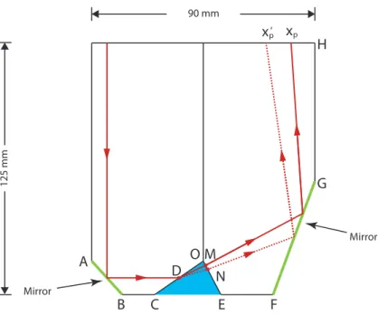
Avec ces deux verres, nous avons conçu un réfractomètre sous la fond d’un bi-prisme (figure 3). Il se compose donc de deux prismes (K7 et N-FK51). Un module laser est utilisé comme source lumineuse pour limiter la bande de longueur d’onde. Un «Position Sensitive Device» (PSD) est choisi pour mesurer la déviation du faisceau laser. Il mesure la position du faisceau laser après réfraction.

Par une méthode géométrique et une méthode différentielle, une relation entre l’indice de réfraction de l’eau de mer et la position du spot laser est obtenue. Basée sur cette relation, la gamme et la sensibilité requise du PSD sont calculées. Si l’indice de réfraction est dans une gamme de 1, 336 (eau douce) à 1, 345 (eau très salée), la longueur du PSD doit être au moins10 mm. Pour atteindre une résolution de 10−7 sur l’indice de réfraction,

(13)

Mirror Mirror A B C O E D F G xp H M xp‘ N

Figure 3: Le principe de réfractomètre «prototype I»

la résolution du PSD doit atteindre 0, 3 µm. Avec ces deux exigences, nous avons choisi un PSD de12 mm avec une résolution étiquetée de 0, 3 µm.

Réalisation d’un réfractomètre à base de PSD

Ensuite, nous assemblons les pièces optiques et optoélectroniques pour fabriquer le réfrac-tomètre. Le processus d’assemblage s’effectue en quatre étapes:

• Collage des blocs optiques • Collage du module laser • Collage du PSD

• Vérification et l’étalonnage

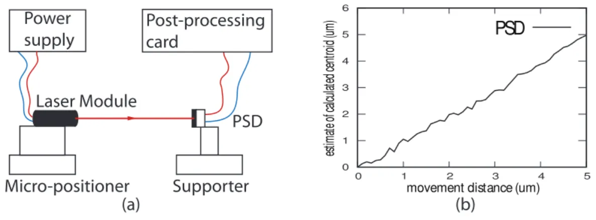
La résolution du réfractomètre dépend de la sensibilité du PSD. Bien que la résolution annoncée soit de 0, 3 µm, la résolution réelle peut être meilleure ou pire que cette valeur. Il est nécessaire d’évaluer la résolution réelle du PSD. Nous avons conçu pour cela un montage de haute résolution (Fig. 4).

(a) (b) Power supply Micro-positioner Supporter Laser Module PSD Post-processing card 0 1 2 3 4 5 6 0 1 2 3 4 5

movement distance (um)

PSD

estimate of calculated centroid (um)

(14)

Le module laser est monté sur un micro-positionneur à 3-dimension avec une résolution de0, 1 µm. Le faisceau laser pointe directement sur le PSD. Les signaux du PSD sont acquis par un ordinateur lorsque le faisceau laser se déplace sur une distance de 50 pas. Selon les résultats, la résolution expérimentale du PSD est de0, 11 µm, la résolution de l’indice de réfraction correspondant est3_{× 10}−7_{, équivalent à la salinité absolue de} _{1 mg.kg}−1_.

Limitation du PSD

Le PSD est un capteur de haute performance pour mesurer la position de la lumière dans l’eau claire. Cependant, dans l’eau turbide, la lumière est diffusée hors de la direction transmise, et la distribution de la lumière est changée. Cette distribution contient beau-coup d’informations, telles que la position du spot laser. Toutefois, le PSD est conçu pour mesurer la position du spot laser, il ne peut pas être utilisé pour mesurer l’intensité lu-mineuse. Cela rend les techniques de post-traitement difficiles. Pour récupérer ces informa-tions, par exemple, la turbidité de l’eau de mer, il est nécessaire d’utiliser un detecteur pour enregistrer la distribution d’intensité lumineuse, par exemple, un CCD (Charge-Coupled Device). Avant de commencer à mesurer les propriétés de distribution connexes, nous avons besoin de prouver que le réfractomètre équipé d’un CCD peut obtenir au moins la même résolution que le réfractomètre équipé d’un PSD.

Le réfractomètre à base de CCD: prêt à construire un capteur

multi-fonctionnel

Principe du réfractomètre avec CCD

Le CCD n’enregistre que la distribution d’intensité de la lumière, il a besoin d’un algorithme de post-traitement pour récupérer les informations. L’algorithme qui peut nous fournir l’information du spot laser s’appelle «image location algorithm». Basé sur des définitions différentes, il existe 3 algorithmes:

• L’algorithme recherche du «centre de gravité» • L’algorithme «transformée de Fourier»

• L’algorithme «détection du bord»

Tous les algorithmes permettent d’obtenir une résolution sub-pixel. Puisque nous voulons comparer les réfractomètres à base de PSD et CCD, l’algorithme de centroïde est utilisé car il mesure le centre de la gravité de l’intensité du spot comme le PSD.

Analyse de performance

La résolution du réfractomètre basé sur CCD est liée a l’erreur systématique. La pre-mière erreur systématique est provoquée par l’échantillonnage, la quantification du CCD, et l’algorithme de gravité. Cette erreur ne peut pas être évitée, mais peut être corrigée. Une autre erreur est provoquée par les bruits. Il y a trois sortes de bruits:

• Bruit de lecture (affecte tous les pixels) • Bruit de fond (affecte tous les pixels)

(15)

• Bruit photonique liée à l’intensité de la lumière incidente.

L’image capturée par le CCD est la somme des bruits et du spot original. L’algorithme de calcul du centre de gravité calcule la position du centre du spot et des bruits. Pour éliminer ou réduire les bruits de lecture et de fond, un seuil ou plusieurs images peuvent être utilisés. Le bruit photonique peut être réduits en appliquant un filtre passe-bas à l’image.

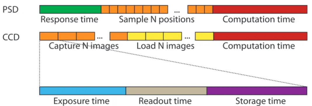
La vitesse est un autre indicateur de performance. Le réfractomètre basé sur l’utilisation d’un PSD a un temps de réponse très court. Toutefois, pour obtenir une résolution élevée, des signaux multiples doivent être capturés. La vitesse du système à base de PSD dépend de la fréquence d’échantillonnage. Le réfractomètre basé sur l’utilisation d’un CCD est plus compliqué. Pour parvenir à haute résolution, des images multiples doivent d’abord être capturées et mémorisées dans un dispositif de stockage, par exemple, le disque dur. L’algorithme doit charger ces images, et puis calculer la position. En conclusion, la vitesse du système à base de CCD dépend du nombre d’images traitées et de la taille de l’image. La saturation du CCD est définie comme le montant maximum des charges qu’un pixel peut recueillir. Quand un pixel atteint ce niveau, la lumière reçue et les charges converties ne satisfont pas une relation linéaire. De plus, les charges qui ne peuvent pas être transférées vont polluer les pixels adjacents et former un «blooming». Pour cette raison, la saturation doit être évitée lors de la mesure.

L’évaluation des paramètres

Avant de commencer à comparer ces deux types de réfractomètres, nous avons besoin d’évaluer les paramètres du réfractomètre basé sur l’utilisation du CCD:

• nombre d’images traitées. • seuil

• taille de la fenêtre • puissance de la lumière

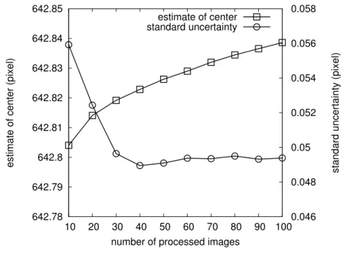
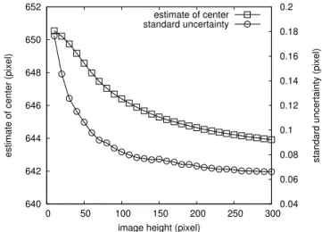
Nous avons fait une expérimentation pour évaluer ces paramètres. Dans l’expérimentation, la position du module laser est fixe et il pointe directement sur le CCD.5 000 images sont capturées pour calculer la référence du centre et celle de la taille du spot. Le niveau de bruits peut être également obtenu par ces 5 000 images: soit 9 (valeur de pixel).

Selon les résultats expérimentaux, nous pouvons déduire les paramètres optimisés pour l’utilisation du CCD. Le nombre d’images traitées est un paramètre critique pour la vitesse, mais pas critique pour la résolution. Le seuil doit être supérieur au niveau de bruit. La taille de la fenêtre «image» est un paramètre critique pour la résolution et la vitesse. Pour obtenir une bonne résolution, la taille de la fenêtre doit être plus grande que la taille du spot. Pour réduire l’erreur systématique, la saturation doit absolument être évitée lors de la mesure.

Comparaison entre les solutions - CCD et PSD

Avec les paramètres optimisés, nous avons conçu une expérimentation pour comparer les systèmes CCD et PSD. Le module laser est monté sur un micro-positionneur à 3-dimensions

(16)

avec une résolution de0, 1 µm. Pour mettre les deux systèmes dans les mêmes conditions, le CCD utilise seulement une fenêtre de267 pixels, soit 1 mm, égale à la hauteur du PSD. Cinq zones sont choisies pour mettre en oeuvre les comparaisons. Dans chaque zone, le module laser est déplacé d’une distance de5 µm par le micro-positionneur avec une pas de 0, 1 µm. Dans chaque étape, 64 images sont capturées en 1 seconde, et le centre est calculé à partir de la moyenne des 64 centres de l’image. Pour le réfractomètre à base de PSD, 10 000 échantillons sont acquis avec une fréquence de 10 000 Hz. La position est calculée par la moyenne de ces10 000 échantillons.

0 0.02 0.04 0.06 0.08 0.1 0.12 0.14 0.16 0 0.5 1

standard uncertainty (um)

measurement zones

CCD PSD

Figure 5: Résultats expérimentaux pour la comparaison entre les systèmes basés sur CCD et PSD

La figure 5 montre les résultats expérimentaux pour la comparaison entre les solutions CCD et PSD. Pour chaque zone, la solution CCD (0, 07 µm) a une meilleure résolution que la solution PSD (0, 11 µm). Il faut noter que la résolution du système à base de PSD repose sur la position du spot. Plus il est loin du centre, plus la résolution est mauvaise. Par contre, la solution CCD est indépendante de la position du spot.

La mesure de turbidité basée sur le réfractomètre

Le réfractomètre à base de CCD peut obtenir une meilleur résolution que le réfractomètre à base de PSD. De plus, le système basé sur CCD peut être utilisé pour mesurer les propriétés liées à la distribution de l’intensité de la lumière en appliquant des algorithmes différents à l’image. Pour prouver l’avantage du système CCD, la mesure de turbidité, sans modifier la configuration de notre réfractomètre, est étudiée dans cette thèse.

La première étape est de choisir les méthodes de mesure de la turbidité. Puisque nous voulons montrer les avantages du post-traitement du CCD, la méthode que nous choisissons doit présenter le moins de modifications possible dans notre réfractomètre. En considérant les méthodes différentes, l’angle de transmission est le bon choix.

Principe de la mesure de turbidité à l’angle de transmission

La figure 6 illustre le principe de la mesure de turbidité à l’angle de transmission. Lorsque la lumière se propage dans un milieu turbide, la lumière est absorbée et diffusée. Il y a

(17)

I0 Itr= I0e−ρ(σa(λ)+σd(λ))l Id Ims Itr+ Ims l

Figure 6: Principe de la mesure de turbidité à l’angle de transmission

trois sortes de lumières. La première appelée lumière transmise Itr peut être calculée par

la formule:

Itr = I0e−ρ(σa(λ)+σd(λ))l (6)

oùρ est la densité de particule, σadécrit la partie de lumière absorbée par une particule

etσa décrit la partie de lumière diffusée hors de la direction transmise. Outre la lumière

transmise, une autre partie de la lumière est diffusée hors de la direction de transmission, et une partie est re-dispersée dans le sens de transmission. Cette dernière partie de lumière s’appelleIms. Selon l’équation 6, la partie ρ(σa(λ) + σd(λ)) et le coefficient d’atténuation,

peut être utilisé pour décrire la turbidité:

T = ln(Im− Ims)− ln(I0)

l (7)

De cette équation, nous pouvons dériver la sensibilité de la mesure de la turbidité. Elle est proportionnelle à la sensibilité du capteur d’intensité lumineuse et inversement proportionnelle à la longueur du chemin parcouru par la lumière dans l’eau. Cette mesure est favorable en milieu à faible turbidité.

L’influence entre la mesure de la turbidité et la mesure de l’indice de réfraction

La lumière diffuse dans toutes les directions dans un milieu turbide. Cela conduit à un problème, la lumière transmise et la lumière diffusée sont mélangées comme on peut le voir dans la figure. 7.

Nous pouvons aussi observer les «speckles» dans l’image ci-dessus, qui sont provoqué par des interférences. Le PSD ne peut pas séparer la lumière transmise de la lumière diffusée. Par conséquence, il ne peut pas être utilisé pour mesurer la turbidité. De plus, la lumière diffusée et les interférences affectent la position du centre de gravité en intensité du spot, ce qui signifie que le PSD ne peut pas fournir la position correctement dans un milieu turbide. Cependant, avec le CCD, il est possible de récupérer le spot d’origine avec le post-traitement des algorithmes. En étudiant la transformée de Fourier de l’image, la lumière diffusée et les interférences existent à hautes fréquences. Une filtre passe-bas d’image permet d’éliminer efficacement les interférences et la lumière diffusée.

(18)

Figure 7: La lumière transmise et la lumière diffusée sont mélangés

(a) (b)

Figure 8: Le spot asymétrique provoqué par la divergence et la diffusion

L’indice de réfraction rencontre un défi en milieu turbide aussi. La divergence du faisceau et la diffusion rendent le spot asymétrique comme on le voit dans la figure 8. Cela conduit à une conséquence que le PSD ne peut pas indiquer la bonne position du spot, et le CCD avec l’algorithme centroïde non plus. Cependant, le CCD peut bénéficier des techniques de post-traitement. Pour résoudre le problème, un nouvel algorithme est développé. Il cherche la position où les parties de deux cotés ont la même masse. En milieu claire, peu importe le nombre de divergences, la position reste au même endroit. En milieu turbide, cette règle fonctionne après avoir éliminé la lumière diffusée par un filtre passe-bas.

En étudiant la position du spot en milieu turbide, nous avons établi une loi de variation de centre: «En milieu turbide, le spot de projection d’un faisceau Gaussien sur une surface avec un angle α est encore un faisceau Gaussien avec la même taille de spot, mais il a un décalage du centre, qui est proportionnel à la turbidité du milieu, la taille du spot, et inversement proportionnelle à la cotangente de l’angle α.»

Pour évaluer les performances de l’algorithme, plusieurs simulations et expérimenta-tions sont réalisées. Le résultat montre que le nouvel algorithme permet d’obtenir une meilleure résolution (0, 035 pixels) que l’algorithme classique (0, 078 pixels) en milieu claire. La résolution du nouvel algorithme est 2 fois plus grande que celle de l’algorithme classique. Plusieurs expérimentations sont réalisées pour évaluer notre méthode de mesure de la turbidité. Les expérimentations ont été menées avec un cube et avec notre réfractomètre. La solution Formazine de 4000 NTU est diluée dans différents échantillons turbides pour calibrer le turbidimètre. Les résultats expérimentaux montrent que la résolution moyenne

(19)

de notre méthode basée sur le réfractomètre atteint 8 NTU dans une gamme de 0 NTU à 200 NTU, et 1,15 NTU dans une gamme de 0 NTU à 20 NTU.Nous avons comparé notre méthode avec le néphélomètre spécifié par le standard. Le résultat calculé par notre méth-ode s’adapte correctement aux résultats obtenus à partir d’un néphélomètre commercial.

Perspective: trois nouveaux prototypes

A la fin de la thèse, nous avons proposé trois nouveaux prototypes de capteur pour mesurer la salinité et la turbidité de l’eau de mer simultanément. Le premier prototype utilise un prisme monobloc pour compenser la variation de longueur d’onde du module laser provoqué par le changement de température. La résolution de la salinité absolue de ce prototype atteint 1, 4 mg.kg−1. Basés sur ce modèle, nous avons ouvert une cavité avec une longueur de 20 mm. Ce prototype a la même résolution de salinité absolue que le précédent. Cependant, la résolution de la turbidité atteint1% de la gamme de mesure. Le dernier prototype a un miroir à45◦ afin de réfléchir la lumière diffusée à90◦. Il est équipé d’une photo-diode pour mesurer l’intensité lumineuse à 90◦. La résolution sur la mesure de turbidité de ce modèle atteint moins de1% de la gamme de mesure.

Conclusion

Le réfractomètre est très bien adapté pour mesurer, avec une très grande précision, la salinité de l’eau de mer. L’utilisation du PSD, dans un premier temps, a permis de mesurer la salinité avec une résolution de1 mg.kg−1. Cependant, le PSD peut seulement travailler en milieu claire, il ne fonctionne pas dans les milieux turbides. Par rapport au PSD, le réfractomètre utilisant un CCD peut être utilisé pour mesurer la salinité et la turbidité en milieu clair et turbide, en appliquant des algorithmes différents à l’image capturée par le CCD. La résolution de mesure de la salinité en utilisant le CCD est meilleur que celle utilisant le PSD. De plus, le système utilisant un CCD a la capacité de mesurer des propriétés différentes de l’eau de mer en appliquant les algorithmes différents.

(20)

Introduction . . . 90 I Review of the turbidity measurement methods . . . 90 I.1 Selection of the turbidity measurement method . . . 91 I.2 Principle of attenuation based method . . . 91 I.3 Attenuation coefficient to turbidity . . . 94 I.4 Sensitivity analysis . . . 95 II Issues in measuring turbidity with refractometer . . . 96 II.1 Measurement distance . . . 96 II.2 Non-uniqueness of light path inside the beam . . . 96 II.3 Light path variation caused by refractive index change . . . 97 II.4 Interference . . . 98 II.5 High turbidity measurement . . . 98 III Issues in measuring refractive index in turbid medium . . . 99 III.1 Non-uniqueness of light path inside the beam . . . 99 III.2 Divergence and scattering caused asymmetrical spot . . . 99 IV Invalidation of PSD . . . 100 V Using CCD to measure the turbidity with refractometer . . . 102 V.1 High turbidity measurement . . . 102 V.2 Scattered light & interference elimination . . . 102 V.3 Solution to light path related problems . . . 103 V.3.1 Light path variation according to the refractive index . . . 103 V.3.2 Non-uniqueness of light path inside the beam . . . 104 V.4 New location algorithm . . . 105 VI Experiments & Results . . . 107 VI.1 Performance evaluation of new location algorithm . . . 107 VI.1.1 Simulation . . . 107 VI.1.2 Experiment . . . 109 VI.2 Simulation & experiments with parallel slab . . . 110 VI.2.1 Simulation . . . 110 VI.2.2 Experiments in high turbid medium . . . 110 VI.2.3 Experiments in low turbid medium . . . 112 VI.3 Simulation & experiments with refractometer . . . 113 VI.3.1 Simulation . . . 113 VI.3.2 Experiments in high turbid medium . . . 113 VI.3.3 Experiments in low turbid medium . . . 115 VI.4 Comparison with nephelometer . . . 115 Conclusion . . . 117 Bibliography . . . 119 Figures and tables . . . 120

5 Perspective: improvements of refracto-turbidi-meter performance 121 Introduction . . . 122 I Issues and Possible improvements . . . 122 I.1 Issues in our methods . . . 122 I.2 Improvements for refractometer . . . 123

(23)

I.3 Improvements for turbidi-meter . . . 124 I.4 Other improvements . . . 125 II Prototype II: new model of refractometer . . . 125 II.1 New model . . . 126 II.2 Performance analysis . . . 126 III Prototype III: new model of refracto-turbidi-meter . . . 127 III.1 Turbidi-meter based on prototype II . . . 128 III.2 Futher improvement . . . 129 Conclusion . . . 131 Bibliography . . . 132 Figures and tables . . . 133

General Conclusion 134

A Algorithm of Seaver & Millard 139

B Resolution analysis of refractometer prototype I 141

C Resolution analysis of refractometer prototype II 145

D Specifications for different prototypes 149

I Specifications for refracto-turbidi-meter prototype I . . . 150 II Specifications for refracto-turbidi-meter prototype II . . . 151 III Specifications for refracto-turbidi-meter prototype III . . . 152 IV Specifications for refracto-turbidi-meter prototype IV . . . 153

(24)

General Introduction

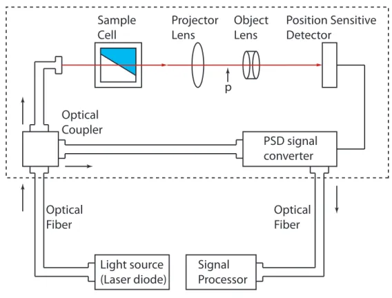
The researches included in this thesis are under the frame of oceanography, which is linked to understanding global climate changes, potential global warming and related biosphere concerns. As a branch of the oceanography, the physical oceanography, which studies the ocean from its physical properties, attracts us the most. Among these oceanographic physical properties, temperature and salinity are two most important ones. In fact, tem-perature, salinity, and pressure are used to calculate density which is directly related to the distribution of horizontal pressure gradients and ocean currents. Another physical property that is important for oceanography is turbidity, which is useful for the oceanog-raphers to study the microorganisms that will participate in the carbon cycle and oxygen production. Changes in temperature, salinity and turbidity help the oceanographers to track the movement of the seawater. For these reasons, we need to know the distribution of temperature, salinity, density, and turbidity in the ocean. This requires different high-resolution measurement instruments to measure these oceanographic physical properties. Current studies have found that all these physical properties are tightly connected to each other to influence the different oceanographic phenomenons, which make the study of in situ multi-functional sensor valuable. Based on these requirements, our research interests is the design of a high resolution multi-functional in situ oceanographic sensor to measure these physical properties, especially salinity and turbidity. Recent researches have built the relationship between salinity and refractive index of seawater. To measure the salinity, a high resolution refractometer is needed. For the turbidity measurement, the scattering property of seawater are studies by different researches and is defined as a represent of turbidity.

The objective of the work described in this document includes the design, modelling, implementation, and improvement of an in situ optical refractometer, which measures re-fractive index of seawater and light attenuation caused by the scattering simultaneously. Specifically, this work is part of a cooperation launched in 2006 between the school TELE-COM Bretagne through the Department optics (UMR FOTON 6082), SHOM (Service Hydrographique et Océanographique de la Marine) and the project NOSS (NkeElectronics Optical Salinity Sensor). The goal is to develop a high resolution and compact optical refractometer to measure the refractive index and light scattering properties of seawater to determine the physico-chemical parameters of the ocean, especially salinity and turbidity. The salinity and turbidity measurement must meet the oceanographic needs, e.g. the mea-sure of salinity must achieve a meamea-surement uncertainty of a few milligrams of salt per litre of seawater. To achieve these resolution requirements, a high resolution refractometer was designed first to measure the refractive index of seawater. Based on the configuration of the refractometer, the possibility of measuring turbidity with the refractometer is discussed and a feasible solution is introduced in this thesis as well. At the end of this thesis, we discuss several methods to improve the performance of the multi-functional in situ optical

(25)

sensor.

The first chapter is for the objective of introducing several necessary definitions to understand the application described in this thesis, different technologies used to measure the physico-chemical ocean parameters, and the state-of-the-art salinity and turbidity mea-surement methods. More precisely, we first introduce the physical oceanography and the principal physico-chemical parameters, especially salinity, conductivity, and turbidity. The Practical Salinity is associated with the conductivity and temperature of seawater, while turbidity is related to the scattering property of seawater. Different salinity and turbidity measurement methods are presented in this chapter as well. Some of these methods can reach high resolution but are hard to integrate into a compact in situ multi-functional sensor, others meet the requirement of integration but have low resolution. That’s why a new high resolution compact in situ multi-functional sensor is studied in this thesis. Our research method is to design a high-resolution salinity sensor first and then add the turbidity measurement functionality into the salinity sensor. By comparing these state-of-the-art salinity measurement methods, the method of refractometer based on the laser beam deviation most fits our requirement and is selected as our basis for the design.

The objective of the second chapter is to introduce the study of design, modelling, and implementation of a high resolution refractometer based on the laser beam deviation measurement. We start from presenting some preliminary knowledge of modelling a re-fractometer, among which we pay special attention to the temperature coefficients of the optical material. Based on these preliminary knowledges, we model the refractometer in both a differential method and a geometrical method to build the relationship between re-fractive index and laser beam deviation. More important, from this relationship we obtain the performance requirements for the geometric parameters and optoelectronic elements in order to reach the desired refractive index resolution (in an order of 10−7_{). To}

ful-fil these requirements, we introduce a high resolution position detection detector (PSD) with a measurement resolution of0.3 µm to measure the laser beam deviation. With the optimized parameters, a detailed operation procedure is included in chapter 2 to guide the fabrication of the refractometer. The last step of the modelling is the verification of the resolution, which recalls an experiment to evaluate the actual resolution of the PSD. According to the experimental result, the resolution of refractive index calculated is about 3_{× 10}−7_{, equals to the absolute salinity of}₁_{× 10}−3 _g.kg−1_.

The third chapter discuss the needed preparation in order to upgrade the high resolution refractometer that we designed into a multi-functional sensor. The transmitted beam carries not only the refractive index related beam deviation information but also the other information associated to the intensity distribution. To obtain these intensity distribution related informations, a pixel-based image sensor is needed to be used to replace PSD, which is designed to calculate the light position. To make this replacement reasonable, it is necessary to prove that by using a pixel-based image sensor, the resolution of laser beam deviation measurement can reach at least the same resolution as the one provided by using a PSD. This chapter first introduces two well-known image sensors, CCD and CMOS. By comparing the technical characteristics of the two image sensors, CCD is selected to be used in the multi-functional sensor. In order to retrieve the laser beam deviation information from the captured images, the centroid algorithm is used to calculate the gravity center of the laser spot. A performance comparison between PSD and CCD combined with a centroid algorithm are discussed with special attention paid to the CCD-based system. According to the operating principle of CCD-based system, several experiments were carried out to evaluate five factors of CCD-based system: image window size, number of processed

(26)

images, threshold, binning and saturation. By applying the optimized parameters, several experiments were made to compare CCD-based system with the state-of-the-art PSD-based system in terms of two performance indicators, namely resolution and speed. It is shown that, by applying the optimized parameters, the performance of a CCD-based system is comparable to that of a PSD-based system in measuring laser beam deviation.

The fourth chapter is aimed at demonstrating the benefits brought from the use of CCD instead of PSD. The measurement of turbidity is one of the best choices for this purpose. In order to best demonstrate the advantages of CCD-based system, we introduce a CCD-based turbidity measurement method in measuring the transmitted light intensity without modifying the configuration of refractometer. By analysing the principle of the turbidity measurement method from measuring the transmitted light intensity, we study the interference between the turbidity measurement and the refractive index measurement. Due to the interference, we further prove that PSD is not suitable to correctly measure neither the refractive index nor the transmitted light intensity in a turbid medium. On the contrary, CCD can overcome the interference and correctly provide both the laser beam deviation information and the transmitted light intensity information in a turbid medium due to the recorded light intensity distribution. To prove the benefits from CCD, a new algorithm and several techniques are proposed to eliminate the interference. Several simu-lations and experiments are carried out to verify the performance of the method proposed in the same chapter.

The last part of the thesis introduces the perspective in the near future and addresses the problem of the turbidity measurement resolution. For this purpose, a new refracto-turbidi-meter is designed under the consideration of both the laser beam deviation mea-surement and the transmitted light intensity meamea-surement. We start from the proposition of several possible ways to improve the performance of the refractive index measurement and the turbidity measurement in a compact sensor. Based on these proposed improve-ment methods, we introduce a new compact in situ double-functional sensor for the salin-ity and turbidsalin-ity measurement of seawater, which has the absolute salinsalin-ity resolution of 1_{× 10}−3_g.kg−1 _{and the turbidity resolution,}_{1% of the measurement range.}

(27)

Chapter 1

State of the art: the measurement of

sea water salinity and turbidity

Contents

Introduction . . . 9 I Generality . . . 9 I.1 Oceanography . . . 9 I.2 Salinity . . . 10 I.2.1 Definition of salinity . . . 10 I.2.2 Absolute Salinity and Practical Salinity . . . 12 I.3 Turbidity . . . 12 I.3.1 Definition of turbidity . . . 12 I.3.2 Scattering . . . 13 I.3.3 Turbidity Standards . . . 15 II Salinity measurement methods . . . 17 II.1 Conductivity based salinity measurement . . . 17 II.1.1 Definition of conductivity . . . 17 II.1.2 Conductivity of seawater . . . 18 II.1.3 Conductivity sensors . . . 19 II.2 Refractometer based salinity measurement . . . 20 II.3 Some refractive index measurement methods . . . 21 II.3.1 Refractometer based methods . . . 21 II.3.2 Interferometer based methods . . . 23 II.3.3 Fiber Bragg grating based methods . . . 24 III Turbidity measurement methods . . . 26 III.1 Transmissometer . . . 27 III.2 Backscatter method . . . 27 III.3 Nephelometric (90◦) scatter method . . . 28 III.4 Multi-angle method . . . 30 Conclusion . . . 32 Bibliography . . . 35 Figures and tables . . . 36

(28)

Introduction

The objective of the work described in this document includes the design, modelling, im-plementation, and improvement of an in situ optical refractometer, which measures the refractive index of seawater and the light attenuation caused by the scattering simultane-ously. The measurement of refractive index is aimed at measuring the salinity, while the measurement of light attenuation is for the measure of turbidity.

This chapter introduces some useful physiochemical properties in the domain of oceanog-raphy, especially salinity and turbidity of seawater. Different principles and methods to measure these two properties, including the most state of the art methods are mentioned in this chapter as well.

At the beginning of this chapter, we give a general introduction of the oceanography and introduce several important seawater properties. Among them, we pay special atten-tion to two of the properties, salinity and turbidity, by describing their definiatten-tions and discussing several methods with their basic principles to measure these two seawater prop-erties. For the introduction of the salinity measurement, the state of the art refractometer are introduced as well. To link the measurement of refractive index to the measurement of salinity, the relationship between seawater refractive index and salinity is illustrated.

The second part of this chapter introduces the state of the art turbidity measure-ment. The scattering theory, which explained the turbidity phenomenon, is firstly reviewed. Based on the theory, several industry turbidity standards are introduced to illustrate the turbidity unit. At the end of this part, we introduce different state of the art turbidity measurement methods.

I

Generality

I.1 Oceanography

Oceanography is a branch of earth science that studies the ocean. It covers a wide range of topics and is divided into several sub-branches, eg. biological oceanography, chemical oceanography, geological oceanography, and physical oceanography. The study of the oceans is linked to understanding global climate changes, potential global warming and related biosphere concerns. Among these sub-branches, we pay special attention to the physical oceanography, which studies the physical properties and dynamics of the ocean. The primary interests are the interaction of the ocean with the atmosphere, the oceanic heat budget, water mass formation, currents, and coastal dynamics[1].

Among the physical properties, four of them, named as temperature, pressure, salinity, and density, are very important to the oceanography. Heat fluxes, evaporation, rain, river inflow, and freezing and melting of sea ice all influence the distribution of temperature and salinity at the ocean’s surface. The changes in temperature and salinity can change the density of the water, which can lead to convection. In addition, temperature, salinity, and pressure are used to calculate density. The distribution of density inside the ocean is directly related to the distribution of horizontal pressure gradients and ocean currents. Density currents are produced where gravity acts upon a density difference between one fluid and another. Besides these four properties, another property named turbidity, which is related to the suspended particles in seawater is very important for oceanography, especially the biological researches. In this thesis, we introduce a double optical sensor to measure salinity and turbidity of seawater.

(29)

I.2 Salinity

Salinity is a very important property to describe sea water, especially associated to the measurement of temperature. Different seas have quite different salinities, for example, the Mediterranean (38-39), the Red Sea (36-47), the Baltic Sea (<15), and the Black Sea (18-22). The salinity map Fig 1.1 shows the areas of high salinity (36) in green, medium salinity in blue (35), and low salinity (34) in purple. Salinity is rather stable but areas in the North Atlantic, South Atlantic, South Pacific, Indian Ocean, Arabian Sea, Red Sea, and Mediterranean Sea tend to be a little high (green). Areas near Antarctica, the Arctic Ocean, Southeast Asia, and the West Coast of North and Central America tend to be a little low (purple).

Figure 1.1: Salinity map of the world

The accuracy of measuring salinity depends on the application. To understand the circulation of seawater in coastal and offshore by measuring the dissolved substances, the accuracy of salinity measurement need to be compatible to the study. For the coastal seawater salinity measurement (less then 600 meters), the required accuracy of salinity in the range of 0 and 38 PSU is _{±0.02 PSU. For the offshore measurement, the expected} accuracy reaches _{±0.003 PSU in a range from 10 to 38 PSU with the depth more than} 2500 meters.

I.2.1 Definition of salinity

In 1865, Fochhammer[2] first introduced the term salinity[3]. In his paper, the salinity is represented as the dissolved salt content of a parcel of water. However, this quantity is not precise enough to measure in practice. With the evolution of the measurement technology, other definitions of salinity were proposed. The first precise definition of salinity of seawater is given by Forch, Knudsen and Sørensen[4] in 1902.

“Salinity is the total amount of solid materials in grams contained in one kilogram of seawater when all the carbonate has been converted to oxide, the

(30)

bromine and iodine replaced by chlorine, and all organic matter completely ox-idized ”[5]

This definition is called absolute salinity with the unit ofg/kg. Although this definition is much more precise, it is not possible to measure this quantity directly. Based on the premise of the constancy of ionic ratios in seawater, the International Council for the Ex-ploration of the Sea defined a “chlorinity” that could be determined by s simple volumetric titration using silver nitrate, to be used as a measure of salinity[6]. Chlorinity was defined as:

“the weight in grams (in vacuo) of the chlorides contained in one gram of seawater (likewise measured in vacuo) when all the bromides and iodides have been replaced by chlorides.”

Based on the measurements on samples of seawater from the surface of the Baltic, Mediterranean, Red Seas, and North Atlantic Ocean, salinity can be calculated with the formula:

Sa= 0.03 + 1.805 Cl, (1.1)

where Sa is the salinity andCl expresses the chlorinity. This equation was used from

1902 to 1962. The major inconvenience of this definition shown in Eq 1.1 is the incon-sistency to the definition of salinity. A sample of seawater with no chlorinity has salinity of _{0.03h. As a result, the Joint Panel on Oceanographic Tables and Standards (JPOTS)} proposed a redefinition of absolute salinity as:

Sa= 1.80655 Cl (1.2)

This definition suffered from the fact that still there was no method for coping with the varying chlorinity-salinity-density relationship under conditions of ionic change. It was used since 1962. In 1978, the salinity was redefined another time. To solve the problem of directly measuring the absolute salinity, the Practical Salinity Scale was defined in 1978. It measures the practical salinity with three other properties: temperature, pressure, and seawater conductivity. The precise definition of practical salinity is:

“The Practical Salinity, symbol S, of a sample of sea water, is defined in terms of the ratioK15of the electrical conductivity of the seawater sample at the

temperature of 15 deg C and the pressure of one standard atmosphere, to that of a potassium chloride (KCl) solution, in which the mass fraction of KCl is 32.4356× 10−3_{, at the same temperature and pressure. The} _K

15 value exactly

equal to 1 corresponds, by definition, to a Practical Salinity exactly equal to 35.”[7]

The relation between practical salinity and the ratio K15 is given by:

S = 0.0080_{− 0.1692K}₁₅1/2+ 25.3851K15+ 14.0941K153/2− 7.0261K 2

15+ 2.7081K 5/2 15 (1.3)

This equation is valid for a Practical Salinity from 2 to 40. From the definition, it is obvious that practical salinity is a ratio and strictly no unit should be used but often PSU (Practical Salinity Unit) is added to that value. In this document, we add “PSU” after the value of practical salinity for clearly expressing the physical meaning of the value.

(31)

I.2.2 Absolute Salinity and Practical Salinity

It is very important to emphasize that the practical salinity does not directly reflect the dissolved salt material in seawater. The total mass of dissolved material, absolute salinity Sa with the unit of g/kg, can be calculated from the equation Sa = a + b S, where a and

b are two coefficients obtained from the seawater samples over the world. In 2006, Jackett and his colleagues[8] gives a more accurate expression of the relationship between absolute salinity and practical salinity by comparing different ocean seawaters as shown in Eq. 1.4.

Sa= (1.0045± 0.0005) S (1.4)

The difference between S andSais approximately0.45±0.05%; for example, a seawater

parcel with S = 35 PSU has an absolute salinity Sa of between 35.140 and 35.175 h, a

difference of approximately 0.16 _{h, which is between 50 and 100 times as large as the} accuracy with which we can determine salinity at sea.

In 2009, the Intergovernmental Oceanographic Commission adopted TEOS-10[9] (Ther-modynamic Equation Of Seawater - 2010) to replace EOS-80 as the official description of seawater and ice properties in marine science. The Absolute Salinity is redefined in TEOS-10 as “Density Salinity” Sdens

A , which is:

“the value of the salinity argument of the TEOS-10 expression for density which gives the sample’s actual measured density at the temperature t = 25◦C and at the sea pressurep = 0 dbar”.

When there is no risk of confusion, “Density Salinity” is also called Absolute Salinity with the labelSA, which can be calculated using Practical Salinity, temperature, pressure

and the computer algorithm of McDougall, Jackett and Millero:

SA= SR+ δSA= SA(SP, φ, λ, p), (1.5)

where φ is latitude (degree North), λ is longitude (degree east, ranging from 0◦_{E to}

360◦E), SP is the Practical Salinity, whilep is sea pressure and δSAis the salinity anomaly.

NotationSR here stands for the reference composition of seawater, which is defined as:

SR≈ uP SSP where uP S≡ (35.16504/35) g.kg−1 (1.6)

According to this definition shown in Equation 1.5, the Absolute Salinity can be ac-curately measured in laboratory. For the applications, which need the highest accuracy, long-term stability and world-wide comparability of the measured values, the only way to obtain high reliability is by traceability of the measurement results to the primary standards of the International System of Units (SI). From these primary standards, the salinity can be computed via an empirical relation that is very precisely known. The UNESCO/IOC SCOR/IAPSO working group 127 (WG127) proposed several potential candidates for this purpose, one of which is the refractive index.

I.3 Turbidity

I.3.1 Definition of turbidity

Besides the salinity, another important property of seawater is the presence of dispersed, suspended solids - particles not in true solution and often including silt, clay, algae and

(32)

other micro-organisms, organic matter and other minute particles. These particles obstruct the transmittance of light through water and impart a qualitative characteristic, called turbidity. The American Public Health Association (APHA) defines turbidity as:

“Turbidity is an expression of the optical property that causes light to be scat-tered and absorbed rather than transmitted in straight line through the sample.” [10]

Figure 1.2: Samples of turbidity

Visually, turbidity affects the clarity of water, the measurement of turbidity is a mea-sure of the relative clarity of water. Fig 1.2 shows the different clarity of water with different turbidity. From the definition of turbidity, it is easy to find out the measurement of turbidity is not a direct measure of suspended particles but, instead, a measure of the scattering effect such particles have on light[11]. The scattering effect is the interaction between light and suspended particles. When light is incident on a particle, several pro-cesses occur, including reflection, refraction, diffraction and absorption. For particles that are of the order of the wavelength in size or smaller, these processes are referred to as “scattering”. Scattering exists not only in the suspended particles but also the molecules of water. Therefore, there is no solution has a zero turbidity, that’s why the measurement of turbidity is a measure of relative clarity of water rather than the absolute clarity.

I.3.2 Scattering

The basic scattering is the scattering of one single particle. When a directed light meets a particle, one portion of the light is absorbed by the particle, while another portion of light is diffused in all directions. The portion of light flux diffused in different directions is defined by the phase function, denoted as p(ˆs0, ˆs), which represents the portion of light flux diffused from direction s to direction ˆˆ s0. The phase function is related to the size, shape and composition of the particle and to the wavelength of the incident light. Since the phase function is related to the size of the particle and the wavelength of the incident

(33)

Figure 1.3: Profile of scattered intensity from particles of three sizes

light, a normalized radiusR = 2πr_λ was introduced to define the size of the particler with respect to the wavelengthλ. The different scattering patterns from particles of three sizes are depicted in Fig 1.3. The left diagram shows the scattering pattern when the normalized radius R 1. In this case, the scattered lights are symmetrically identical in forward and backward. As normalized radius R of particle increases, light scattered from different points of the particle create interference patterns that are addictive in the forward direction. This makes the forward-scattered light greater than the backward-scattered light. The middle diagram of Fig 1.3 shows the scattering pattern of a large particle, while the right one is the scattering pattern of a larger particle.

Figure 1.4: Example of 3D Mie scattering angular pattern

Beside the size of particle, the shape and refractive index of particle affect the shape function as well. The scattering distribution of spherical particle is well studied by Gus-tav Mie[12], who gave an analytical solution of Maxwell’s equations for the scattering of electromagnetic radiation by a single spherical particle. This theory is then called the Mie theory. Fig 1.4 is the 3D Mie scattering angular pattern of a particle with radius 2 µm, when a 633 nm incident light passing through it from the left. Special case of the Mie

(34)

scattering is the Rayleigh scattering, named after the British physicist Lord Rayleigh, is the elastic scattering of light or other electromagnetic radiation by particles much smaller than the wavelength of the light. The particles may be individual atoms or molecules[13]. The left diagram of Fig 1.3 is one example of Rayleigh scattering. In order for scattering to occur, the refractive index of particle must be different than the refractive index of sample liquid. Since the particle’s refractive index determines how it redirects the light passing through it, the scattering becomes more intense when the difference between the particle’s refractive index and the refractive index of sample liquid increases.

Another coefficient that impacts the scattering effect is the color of the suspended solids and the sample liquid, because the colored suspended solids and sample liquid absorb light in certain bands of the visible spectrum. This results in the decrease of both the transmitted light and scattered light.

Figure 1.5: Multiscattering example

In a volume of water, the scattering happens in all the suspended particles that interact with the light, thus the total scattered light increases as the number of particle increases. However, this rule is broken when the number of particles exceeds a certain point. For a volume of water with high particle concentration, a scattered light has a high chance to meet another particle to scatter again. This phenomenon is called multi-scattering, shown in Fig 1.5. Multi-scattering acts to reduce the distance traversed by the scattered rays, so that the total scattered light decreases.

I.3.3 Turbidity Standards

Practical attempts to quantify turbidity date to 1900 when Whipple and Jackson[14] devel-oped a standard suspended fluid using 1000 parts per million (ppm) of diatomaceous earth in distilled water. Dilution of this reference suspension resulted in a series of standard sus-pensions used to derive a ppm-silica scale for calibrating contemporary turbidimeters[11]. Jackson invented a turbidimeter with a special candle and a flat-bottomed glass tube, and calibrated it in graduations equivalent to ppm of suspended silica turbidity. This turbidimeter is then called the Jackson Candle Turbidimeter. The usage of the Jackson Candle Turbidimeter is shown in Fig 1.6. A burned candle is putted under the flat-bottomed tube. The measurement is made by slowly pouring a turbid sample into the tube until the visual image of the candle flame, viewed from the open top of the tube, diffused to a uniform glow. The visual image of the flame disappears when the intensity of the scattered light equalled that of transmitted light. The depth of the sample in the

(35)

Figure 1.6: Jackson Candle Turbidimeter

tube was then read against the ppm-silica scale, and turbidity was referred to in terms of Jackson Turbidity Units (JTU).

Jackson Candle Turbidimeter was firstly based on standards prepared from material found in nature, such as Fuller’s earth, kaolin and stream-bed sediment, making consis-tency in formulation difficult to achieve. To improve the consisconsis-tency in formulation, a new suspension for turbidity standards named formazin was developed by Kingsbury and Clark[15] in 1926. It is prepared by accurately weighing and dissolving 5.00 g of hydrazine sulfate and 50.0 g of hexamethylenetetramine in one liter of distilled water. Formazin can be reproducibly prepared from assayed raw materials. Under ideal environmental con-ditions of temperature and light, this formulation can be prepared repeatedly with an accuracy of_{±1%. Formazin was first adopted by the APHA and American Water Works} Association (AWWA) as the primary turbidity standard material in the 13th edition of Standard Methods for the Examination of Water and Wastewater and units of turbidity measurement became known as Formazin Turbidity Units (FTU) .

Even though the consistency of formazin improved the accuracy of the Jackson Candle Turbidimeter, it was still limited in its ability to measure extremely high or low turbidity. What is more, it is dependent on human judgement to determine the exact extinction point, which makes it not practical. In addition, the light source of the Jackson Candle