HAL Id: hal-02087291
https://hal.archives-ouvertes.fr/hal-02087291
Submitted on 2 Apr 2019
HAL is a multi-disciplinary open access
archive for the deposit and dissemination of
sci-entific research documents, whether they are
pub-lished or not. The documents may come from
teaching and research institutions in France or
L’archive ouverte pluridisciplinaire HAL, est
destinée au dépôt et à la diffusion de documents
scientifiques de niveau recherche, publiés ou non,
émanant des établissements d’enseignement et de
recherche français ou étrangers, des laboratoires
Modeling of pipeline corrosion degradation mechanism
with a Lévy Process based on ILI (In-Line) inspections
Rafael Amaya-Gómez, Javier Riascos-Ochoa, Felipe Munoz, Emilio
Bastidas-Arteaga, Franck Schoefs, Mauricio Sánchez-Silva
To cite this version:
Rafael Amaya-Gómez, Javier Riascos-Ochoa, Felipe Munoz, Emilio Bastidas-Arteaga, Franck Schoefs,
et al.. Modeling of pipeline corrosion degradation mechanism with a Lévy Process based on ILI
(In-Line) inspections.
International Journal of Pressure Vessels and Piping, Elsevier, In press,
�10.1016/j.ijpvp.2019.03.001�. �hal-02087291�
Modeling of pipeline corrosion degradation mechanism with a
L´evy Process based on ILI (In-Line) Inspections
Rafael Amaya-G´omeza,d,⇤, Javier Riascos-Ochoac, Felipe Mu˜noza, Emilio Bastidas-Arteagad,
Franck Schoefsd, Mauricio S´anchez-Silvab
aChemical Engineering Department, Universidad de los Andes, Cra 1E No. 19A-40, Bogot´a, Colombia bDepartment of Civil & Environmental Engineering, Universidad de los Andes, Cra 1E No. 19A-40, Bogot´a, Colombia
cBasic Sciences Department, Universidad Jorge Tadeo Lozano, Cra 4 No. 22-61, Bogot´a, Colombia dUniversit´e de Nantes, GeM, Institute for Research in Civil and Mechanical Engineering/Sea and Littoral Research
Institute, CNRS UMR 6183/FR 3473, Nantes, France
Abstract
In pipelines, one of the primary testing procedures used to identify the e↵ects and evolution of corrosion over time is through In-Line Inspections (ILI). ILI inspections provide detailed infor-mation regarding the inner and outer pipeline condition based on the remaining wall thickness. Based on this information, di↵erent approaches have been proposed to predict the degradation extent of the defects detected. However, these predictions are subject of uncertainties due to the inspection tool and the degradation process that poses some challenges for assessing an en-tire pipeline within the timespan between two inspections. To address this problem, ILI data was used to formulate a degradation model for steel-pipe degradation based on a Mixed L´evy Process. The model combines a Gamma and Compound Poisson Processes aimed for a better description of the degradation reported by the ILI data. The model seeks to estimate corrosion lifetime distribution and the mean time to failure (MTTF) more accurately. The model was tested on an actual segment of an oil pipeline, and the results have been used to support a preventive maintenance program.
Keywords: Pipeline, corrosion, Mixed degradation process, L´evy Process, Maintenance.
1. Introduction
Corrosion is one of the frequent causes of failure in hydrocarbon pipelines [1, 2]. It fol-lows a progressive degradation process in which the condition of the structure decreases con-tinuously with time. Existing approaches to evaluate corrosion-based degradation include: (i) phenomenological descriptions [3, 4], (ii) random variable adjustments [5, 6], (iii) stochastic processes [7, 8], (iv) simulation processes [9, 10], (v) empirical approaches [11, 12], and (v) de-terministic approaches [13]. Considering any of these degradation processes, the main challenge of a corrosion assessment lies in predict the condition of the pipeline between scheduled inspec-tions to prevent any possible failure. Considering the nature of the transporting fluids, a loss of
⇤Corresponding author, Tel. (+57-1) 3394949 Ext.3095
Email address: r.amaya29@uniandes.edu.co (Rafael Amaya-G´omez)
Preprint submitted to International Journal of Pressure Vessels and Piping February 12, 2019
Please cite this paper as:
Amaya-Gómez R, Riascos-Ochoa J, Muñoz F, Bastidas-Arteaga E, Schoefs F, Sánchez-Silva M. (2019).
Modeling of pipeline corrosion degradation mechanism with a Lévy Process based on ILI (In-Line) Inspections.
International Journal of Pressure Vessels and Piping, In press https://doi.org/10.1016/j.ijpvp.2019.03.001
containment may lead to human, environmental or economic losses. An important challenge re-lies on accounting for several factors that impact corrosion evolution, among them: current state, temperature, degradation initiation, and chemical composition of the steel.
For this purpose, pipeline integrity management practices such as the definition of inspection-repair strategies and failure analysis are commonly implemented. Within these practices, In-Line Inspection (ILI) assessment (NACE RP0102-2002 Standard) is a non-destructive technique often used to establish a clear perspective of the inner and outer condition of the pipe using magnetic (MFL) or ultrasonic (UT) tools to identify and measure metal loss. This analysis is commonly preferred from other acceptable methods reported in the Code of Federal Regulation for Liquids and Gases (CFR 192 and 195) to assess the mechanical integrity of pipelines [14]. The results of an ILI inspection are central to define a maintenance policy based on the pipeline condition [7, 15–17]. Overall, these policies seek to minimize the total expected life-cycle costs (i.e., construction, inspections, failures, and repairs) based on continuous degradation models.
Detailed assessments for long pipelines poses some restrictions on the selection of the eval-uation tool. For instance, phenomenological approaches such as Computational Fluid Dynamics (CFD) or finite element analysis (FEM) require significant computational resources, which make impossible to assess all detectable defects in a system. Empirical and deterministic approaches do not capture the evolution of degradation mechanisms and their corresponding uncertainties. Sim-ulation approaches such as Neural Networks require previous knowledge of distributions or data and lead to significant computational cost. Within this context, a stochastic based degradation can be used in advance as a way to handle both the degradation mechanism and the uncertainties associated with the ILI measurements.
Stochastic processes are justified by the fact that modeling degradation is a time-dependent process, which is uncertain by nature. The first approach in this direction corresponds to the use of Markov Chain processes. Some examples of this approximation include: (i) a model of the corrosion defect’s e↵ect on the remaining pipeline strength [18] and (ii) a model for pitting corrosion using non-homogeneous linear growth Markov process [19]. A second approach is the use of Gamma Processes as in Zhou et al. [20], in order to evaluate time-dependent pipeline reli-ability based on multiple active corrosion defects. This process has shown interesting results for predicting degradation in steel structures and life-cycle performance analyses [21, 22]. Finally, the use of L´evy Processes has attracted much attention recently [23, 24]. Based on a L´evy subor-dinator (i.e., increasing sample paths) as a Compound Poisson Process, degradation mechanisms can be best-described [23]. Recently, Riascos-Ochoa et al. [24] developed a model following a L´evy Process based on multiple degradation sources, which is then used to determine the Mean Time to Failure (MTTF) and Reliability by analytical expressions. In this work, this approach is used to assess the corrosion degradation process.
The objective of this paper is to present a stochastic characterization of a corrosion degra-dation process, which incorporates both the physical mechanism and associated uncertainties, with the aim to support operational decisions. The document is structured as follows: Section 2 presents a description of the evaluation of a pipeline performance over time. Section 3 describes the available degradation models for a corroded pipeline. Section 4 describes the proposed ap-proach for modeling and assessing the reported corrosion. Section 5 presents the description of the case study; the results and discussion are shown in Section 6; and finally conclusions are given in Section 7.
2. Evaluation of pipeline performance over time 2.1. Inspection framework and underlying uncertainties
According to the Pipeline Operators Forum (POF), the result of an ILI inspection contains a pipe tally, list of anomalies, and a list of clusters [25]. The pipe tally presents a list of all pipeline and anomaly features, which include: (i) Location and orientation parameters, (ii) struc-tural parameters, and (iii) information regarding anomalies. The list of anomalies describes the anomalies found with the inspection tool concerning their geometric extent (i.e., width, length, and depth), location, and orientation using a clock-position analogy (Fig. 1). Finally, a defect-cluster classification is provided in the list of defects considering the ASMEB31G criterion [25].
00:00 hr 06:00 hr 09:00 hr 03:00 hr 12:00 hr Defect length D e fe c t w idt h Pipeline abscissa C loc k -p os iti on Defect center Pipeline wall thickness (t) Remaining Wall thickness
Depth of metal loss (d)
Deepest point (dmax) Measurement threshold Abscissa 00:00 hr 03:00 hr 06:00 hr 09:00 hr
Figure 1: Scheme of the location of a corrosion defect. Modified from [25].
Specifically for metal loss assessment, ILI inspections capture information using Magnetic Flux Leakage (MFL) or Ultrasonic (UT) tools. The MFL tool induces a magnetic flux on the pipe wall seeking for flux leakages when the PIG (Pipeline Inspection Gauge) crosses the pipe. Based on the shape and amplitude of the signal, the nature of the anomaly can be estimated. The UT tool uses the time-elapsing reflexion and the angle of ultrasound waves to detect the metal loss [26]. As any other inspection tool, these techniques are subject to limitations detecting and measuring the corrosion defects on the pipe wall. For instance, MFL tools are primarily sensitive to the depth and the circumferential extent of an anomaly. However, long narrow areas of metal loss or axial cracks cannot be detected because the flux field is parallel to the length of the anomaly and the flux is not pushed outside of the wall thickness [26]. About the UT tool, several types of flaws including cracks or material separation are also detected [26], but this tool does not detect cracks with a length shorter than 30 mm or corrosion defects with a depth shorter than 2 mm [27].
Based on the inspection tool, each defect can be classified as detected or non-detected based on reporting thresholds that depend on the geometry of the defect (usually the depth). However, this detection process goes beyond a threshold that discriminates whether a defect is detected or not. Indeed, there is a probability that a sensor detects a defect (PoD- Probability of detection) or to be just a False Alarm (PFA-Probability of false alarm). This probability is relevant because it can be used as reporting threshold when information about the tool is not available [25] For this purpose, an exponential function is commonly used to describe the probability of detection based on the defect size and the accuracy of the inspection tool:
PoD(d) = 1 exp( qd) (1)
where d is the defect depth and 1/q is the average depth of defects that are detected [28]. Ku-niewski et al. [29] proposed another approach to estimate this probability of detection. Based on laboratory hit-miss data, they suggested a fit with a log-logistic regression model with the following shape:
PoD(d) = exp(b0+b1ln(d))
1 + exp(b0+b1ln(d)) (2)
where b02 R and b1>0 are the fitting parameters.
Besides the PoD, the inspection results are delimited by the resolution of the inspection tool regarding the location and sizing of the defects. Table 1 illustrates the resolution from the prin-cipal measurement parameters reported by the Pipeline Operator Forum.
Table 1: Resolution of measurement parameters [25]. Parameter SI unitsResolution/AccuracyAlternative units
Abscissa 0.001 m 0.1 in
Defect length and width 1mm 0.01 in Defect depth 0.1 mm or 1% 0.01 in or 1% Reference wall thickness 0.1 mm or 1% 0.01 in or 1%
Orientation 0.5 C 1 minute
Temperature 1 C 1 F
Regarding defects dimension uncertainties, several authors have proposed random scattering er-rors associated with the ILI-reported dimensions, commonly normally distributed [6, 30, 31], and location uncertainties are associated with the inspection tool capabilities. ILI inspection contrac-tor commonly provides information of the location and orientation capabilities of the inspection tool, namely, the axial position accuracy (in meters) and the circumferential position accuracy (in degrees).
2.2. Reliability problem formulation
Consider a system that starts operating at t = 0 and whose condition or capacity decreases with time. Denote this dependent time capacity at time t as Vt and let Vo denotes the initial
capacity (i.e., at t = 0). The accumulated degradation at time t is described by a random variable Xt. In the case of pipelines, this condition can correspond to the remaining wall thickness. If
the system is assumed to be abandoned after the first failure (i.e., without any maintenance), the system’s condition at time t can be computed as [32]:
Vt=max{Vo Xt,0} (3)
The system failure occurs when its state falls below a predetermined ultimate or operational threshold k⇤, where 0 < k⇤ <V0. An ultimate threshold corresponds to the case in which the
system is unable to fulfill its function; for instance, the entire wall thickness of a pipeline. An operational threshold describes a minimum acceptable operative condition such as plastic defor-mation or a corrosion defect-depth of 80% of pipeline wall thickness. Depending on the imple-mented threshold, di↵erent possible interventions decisions can be supported. For instance, an ultimate threshold indicates that the system must be replaced, whereas an operational threshold suggests a preventive maintenance [33].
The following random variable can estimate the lifetime or the time in which the failure occurs:
L = inf{t 0 : Vt k⇤} = inf{t 0 : Xt V0 k⇤} (4)
where MTTF= E[L], the reliability function is R(t) = P(L > t) = P(Vt k⇤) = P(Xt V0 k⇤),
and the failure probability writes Pf(t) = 1 R(t).
2.3. Degradation mechanisms
Degradation processes Xtare usually divided into three main categories: (i) shock-based, (ii)
progressive, and (iii) combined degradation [24, 32, 33]. A shock-based degradation process occurs when discrete amounts of the system’s capacity are removed at distinct points in time due to sudden and independent events (e.g., earthquakes). These shocks are assumed to occur randomly over time accordingly to some physical mechanism, and two stochastic processes de-scribe them: (i) inter-arrival time between shocks {Ti}1i and (ii) the damage of each shock {Yi}1i .
A particular case of a shock-based mechanism is a Compound Poisson Process (CPP), whose Ti are iid distributed exponentially. A progressive degradation (graceful) process is the result
of the capacity being continuously reduced at a rate that may change over time. It is generally the result of a mechanical process based on internal or external conditions and can be described as a deterministic function rate or by progressive degradation jumps [33]. Finally, a combined degradation includes both processes. In what follows, some of the main stochastic approaches used to model the degradation process associated with corrosion will be presented.
3. Degradation models
Corrosion is a progressive degradation mechanism. Stochastic processes commonly used to model it are: the Gamma Process (GP) and the Inverse Gaussian Process (IGP). These are jump-processes with independent increments. The jumps are non-negative and happen infinitely often in any finite time interval, properties that makes these processes suitable to model progressive degradation. In fact in most cases, corrosion defects can be modeled rather accurately using a gamma distribution [5, 17, 20, 34, 35]. In what follows, the basic properties of these processes are briefly described below.
3.1. Gamma Process-based approach
According to van Noortwijk [36], a GP, {Xt}t 0, is a continuous stochastic process with the
following properties: (i) X0=0 with probability one, (ii) X⌧ Xt⇠ Ga(v(⌧) v(t), u) for ⌧ > t 0,
and (iii) Xthas independent increments. Here Ga(·, ·) denotes the gamma distribution given by:
Ga(x|v, u) = u(v)v x(v 1)e uxI
(0,1)(x) (5)
where v and u > 0 are the shape and scale parameters, I(0,1)is the indicator function, and (v)
is the Gamma function for v > 0. For the GP, v(t) is non-decreasing function with continuous real values and v(0) = 0, which can be associated with a power law v(t) = ctb where c, b > 0
with a constant parameters b for corrosion modeling [37]. These parameters are commonly de-termined by statistical methods such as maximum likelihood and method of moments [36]. The GP lifetime can be expressed by the incomplete gamma function (i.e., (a, x) =Rt=x1t(a 1)e tdt)
as follows [37]:
F(t) = P(L t) = P(Xt Vo k⇤) = (v(t), (Vo k ⇤)u)
(v(t)) (6)
The lifetime probability density function (pdf ) is obtained using the chain rule, assuming that v(t) is di↵erentiable [36]: f (t) = v 0 (t) (v(t)) Z 1 (Vo k⇤)u ⇥log(z) (v(t))⇤zv(t) 1e zdz (7)
where the function (a) corresponds to the digamma function. 3.2. Inverse Gaussian Process-based approach
The inverse Gaussian Process (IGP) is one of the stochastic processes recently implemented to model degradation processes [31, 38–41]. The IGP is a process with independent increments following an Inverse Gaussian distribution. It has the following properties [31]: (i) X0 =0 with probability one, (ii) X⌧ Xt follows an inverse Gaussian distribution with pdf: fX⌧ Xt(x⌧ xt |
⇤⌧ ⇤t, ⇣(⇤⌧ ⇤t)2), and (iii) {Xt}1t has independent increments.
If the mean of the distribution is denoted as µ > 0 and the shape parameter is denoted as ✓ >0, then the IGP probability density function for a random variable X is given by [31]:
fX(x | µ, ✓) = r ✓ 2⇡x3 exp ✓(x µ)2 2µ2x ! , x > 0 The corresponding variance for this pdf is given by µ3/✓. Now, let {X
t}t 0be a IGP over a time t.
Then a parametrization with a mean function ⇤t=E[Xt] and a shape function ⇣(⇤t)2, where ⇣ is
a scale parameter, obtain the pdf of the IGP process as follows [31, 41]:
fXt ⇣ xt| ⇤t, ⇣(⇤t)2 ⌘ = s ⇣ 2⇡x3 t ⇤texp ⇣(xt ⇤t) 2 2xt ! , xt>0, (8)
which in turn, reaches the following reliability function given a threshold k⇤[41]:
R(t) = P(Xt k⇤| ⇤(t), ⇣) = 2 66664r⇣ k⇤(k⇤ ⇤(t)) 3 77775 + exp{2⇣⇤(t)} 266664 r⇣ k⇤(k⇤+ ⇤(t)) 3 77775.
For monotone degradations such as corrosion, this stochastic process is suitable because the monotonic requirement is inherently ensured. This requirement is completed thanks to the mean function, which is required to be monotonically increasing with time. Some approaches as Qin et al. [39] and Zhang & Zhou [31] suggest a power law function for this purpose:
⇤i j =
8 >><
>>:↵↵ii(t(tjj tti0j 1) ,) , for j = 1for j 2
where ti0is the initiation time of the ithcorrosion defect, tirepresents the time of the ith
inspec-tion, ↵iis the mean growth rate in a unit time, and is a constant that delineate the power law
performance of this function. From the approaches reviewed, this last parameter was set to = 1, which represents a linear trajectory over time [31, 39, 40].
Some variations of the above approaches include: (i) a GP or an IGP with a Gaussian copula (or a sum of GPs or IGPs) to model the degradation of several corrosion defects [40], and (ii) an IGP with random e↵ects to address common heterogeneities (random degradation rate) [38]. In general, these approaches fit the degradation process using the mean and variance (i.e., first two central moments); however, recent results have shown that also the third moment a↵ects the fitting and poses additional challenges for the corrosion predictions [42].
3.3. Mixed process: A L´evy Process approach
One general stochastic process that includes GP and IGP is a L´evy Process, which is defined as follows [24]: Given a filtered probability space (⌦, F , F, P), an adapted process {Xt}1t=0with
X0=0 almost surely (a.s.) is a L´evy process if:
• {Xt}1t has independent increments from the past, namely, Xt Xsis independent from Fs
with 0 s t 1
• {Xt}1t has stationary increments, namely, Xt Xs has the same distribution as Xt s with
0 s t 1.
• Xtis continuous in likelihood, namely, limt!sP(Xt2 ·) = P(Xs2 ·).
Using the L´evy-Ito decomposition theorem, it is possible to describe a L´evy Process as a superposition of three independent processes: (i) deterministic drift, (ii) quadratic Gaussian pro-cess, and (iii) a L´evy measure. Clearly, in the case of systems that degrade continuously, the second component (i.e., Gaussian quadratic part) can be neglected, and the process will still be L´evy. This process can be implemented through the characteristic function and the correspond-ing characteristic exponent of the three main degradation processes that can be described: (i) shock-based, (ii) progressive, and (iii) mixed-based (See Section 2.3).
A shock process, Wt, may be implemented if: (i) the deterministic drift is neglected; and (ii)
the L´evy measure has support on R+and it is finite. Thus, W
t corresponds to a CPP and can
be written as Wt =Pi=1Nt Yi, where Ntis the number of shocks until time t. Consider the shocks
following a Poisson process with rate . A progressive degradation corresponds to the sum of two independent processes: (i) a linear deterministic drift and (ii) a jump process with an infinite L´evy measure, i.e., ⇧Z(R) = 1. The mean and the n-th central moment of Ztwould be given
by the characteristic exponent of the jump process [24]. In the particular case of a GP, consider the shape function of the gamma distribution as v(t) = gt ( g > 0) and a scale parameter
u = g. Finally, a Mixed-L´evy process Kt is defined as the sum of two independent models,
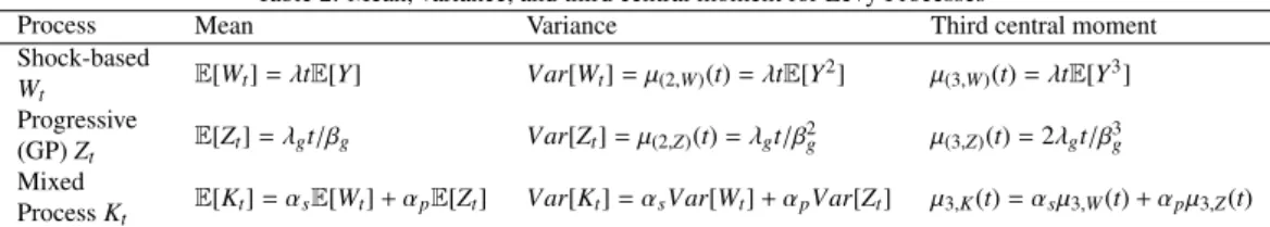
and its characteristic exponent correspond to a linear combination of the constitutive processes. Based on the characteristic function, mean and central moments expressions of the degradation process can be determined by their n-th derivate evaluated at zero. Further details can be found in Riascos-Ochoa et al. [24]. The equations for the mean, variance, and third central moment of each process are summarized in Table 2.
Riascos-Ochoa et al. [24] proposed a numerical solution to obtain the reliability quantities (i.e., lifetime, MTTF, and reliability function) using the inversion formula. Appendix A presents an approach to determine the parameters, which will be later used for modeling corrosion.
Table 2: Mean, variance, and third central moment for L´evy Processes
Process Mean Variance Third central moment
Shock-based
Wt E[Wt] = tE[Y] Var[Wt] = µ(2,W)(t) = tE[Y
2] µ(3,W)(t) = tE[Y3] Progressive (GP) Zt E[Zt] = gt/ g Var[Zt] = µ(2,Z)(t) = gt/ 2 g µ(3,Z)(t) = 2 gt/ 3g Mixed
Process Kt E[Kt] = ↵sE[Wt] + ↵pE[Zt] Var[Kt] = ↵sVar[Wt] + ↵pVar[Zt] µ3,K(t) = ↵sµ3,W(t) + ↵pµ3,Z(t)
4. Approach to corrosion modeling and assessment 4.1. Overview
Overall, data collected with ILI inspections is used as the basis for modeling degradation due to corrosion, which is later used to evaluate the mechanical integrity of the pipeline. After collecting corrosion data from the ILI inspection, a tidying process that focused on the mea-surement of the defects and their location is carried out. Based on this information, a stochastic degradation model that captures the evolution of the corrosion-depth increments at various ILI measurements is constructed, the pipeline integrity is evaluated using the Mean Time to Failure along the abscissa to identify leak-prone segments and the potential spilled volume in case of a LOC to identify potential critical segments. Finally, an Age Replacement Maintenance compar-ison is implemented based on the proposed approach. Fig. 2 illustrates the overall methodology proposed in this work.
Data collection Data tidying process Degradation process selection Maintenance support decision-making Data P roc es si ng Corros ion S toc ha st ic M ode li ng P ipe li ne Int egri ty A ss es sm ent
Mixed Lévy process parameters estimation
Mean Time to Failure (MTTF) Identification of leak-prone segments
Figure 2: General methodology for pipeline degradation assessment.
4.2. Data processing
Assume initially that the ILI inspection tool has a defect location uncertainty denoted as ✏, commonly reported by the inspection vendor. Which means that a defect x = (x1,x2) may be
located within a circular area B✏(x) := {y = (y1,y2) 2 (A ⇥ P) | p(x2 y2)2+(x1 y1)2 ✏},
where (A ⇥ P) is the ordered pair indicating the abscissa and perimeter defect location on the pipeline. This uncertainty is important considering that defects might not be accurately located between two ILI runs. Let’s define S1as the set of depth increments at the exact location between
ILI runs, and S2 as the set of depth increments considering the possibility that there is some
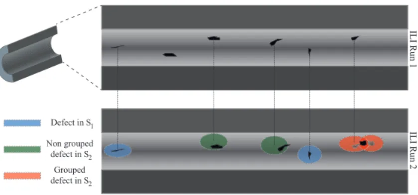
uncertainty in the location of the defect. In the former case, depth increments can be obtained directly from the measurements. However, in the latter case, more than one corrosion defect may be located in these circular regions. In this case, a hypothetical corrosion defect could be defined by the mean or maximum depth of the corrosion defects within each B (Fig. 3).
IL I Run 1 Grouped defect in S IL I Run 2 Defect in S Non grouped defect in S 1 2 2
Figure 3: General S1and S2diagram.
4.3. Stochastic corrosion model
The proposed growth corrosion model is based on the geometric extent of defects, principally on depth-increments. Based on several ILI measurements, the corrosion evolution along the pipeline is determined from defect depth increments between inspections. If there are m detected defects and n ILI measurements, the depth increments i
jof the i-th defect in the j-th inspection
could be obtained by:
x = { 1j, . . . , mj} 8 j 2 2, 3, . . . , n
x = n(x1j x1j 1), . . . , (xmj xmj 1)o 8 j 2 2, 3, . . . , n (9) where xi
j denotes the degradation (e.g., defect depth) of the i-th defect at the j-th ILI
measure-ment. The equations in Section 3 correspond to the degradation process of only one corrosion de-fect, and it should be implemented for each defect to evaluate the integrity of the entire pipeline. Nevertheless, this process may be unfeasible due to their computational cost considering that a pipeline of 45km might have more than 60,000 corrosion defects over a period of 50 years. The latter following the generation of new defects results of Zhang [7]. Therefore, it was assumed that every defect has the same degradation mechanism; the following two alternatives are proposed to determine their degradation parameters:
1. To consider the expected metal loss on the wall thickness on the corrosive location instead of individual corrosion increments (xi
j xij 1).
2. To consider all the corrosion increments (xi
j xij 1) as two hypothetical ILI measurements
with these increments.
In both alternatives, depth-increments are used as input to estimate the parameters. In this work, the latter case is implemented because two ILI measurements were available.
4.3.1. Selection of the degradation mechanisms
Based on the available ILI inspections, the degradation process that best describes its corro-sion mechanism is determined using the Feasible Moments Criterion [24]. This criterion consid-ers the second and third central moments (i.e., µ2(t) and µ3(t)) of the degradation process, which
increase proportionally with time (see Table 2); thus, µ2(t)/t and µ3(t)/t are constant
parame-ters associated with the increasing rates of these moments. This criterion uses the ordered pairs {µ2(t)/t, µ3(t)/t} to select the degradation mechanism that better fits the data. This paper proposes
a Mixed L´evy process composed of a Gamma Process (GP) and a Compound Poisson Process (CPP) upon the results from the Feasible Moments Criterion just mentioned before (see Section 3.3).
Once the mechanisms are selected, the next step is to determine the parameters of these mechanisms. The progressive degradation mechanism follows a Gamma Process, {Zt}t 0, which
is also a L´evy Process, so its parameters can be determined based on the degradation mean and variance (see Appendix A). Note that the reported in Appendix A involve the mean and variance of the corrosion depth-increments, but does not depend on the third central moment, which is a measure of the degradation skewness. Once the parameters of the GP are defined, it remains to determine the shocks size (Y), the shocks time inter-arrival time ( ) of the shock process {Wt}t 0,
and the superposition coefficients (↵s, ↵p), which will depend on the shocks’ distribution. These
parameters are estimated using an optimization model that assumes that a previous moment-matching approach for progressive degradation is already completed (see Appendix A).
4.3.2. Optimization-based model
Consider that the mean and central moments of the shock-based process are described in terms of the shocks size (Y) and their inter-arrival time ( ). Also, assume that the corrosion depth-increments are independent. Then, the parameters can be obtained by minimizing the di↵erence between the third moment of the degradation process with the actual reported data. This optimization should be subjected to fit the mean and second central moment of the depth-increments from the ILI measurements (EILIand µ(2,ILI)):
minimize {↵p,↵s, ,Y} ↵Pµ(3,Zt)+ ↵Sµ(3,Wt) µ(3,ILI) subject to ↵Pµ(2,Zt)+ ↵Sµ(2,Wt) = µ(2,ILI) ↵PEZt+ ↵SEWt =EILI (10)
This approach assures that the degradation process describes the mean and central moments of the corrosion defects-depth increments completely.
4.4. Pipeline integrity assessment
Pipeline integrity comprises concepts of failure prevention, inspection, and repair, including products, practices, and services that help operators maximize their assets. Pipeline integrity evaluation is a problem commonly addressed in standards such as API579 (Fitness-For-Service), ASME B318S (Managing System Integrity of Gas Pipelines) and API1160 (Managing system
integrity for hazardous liquid pipelines). The main practices regarding pipeline integrity man-agement can be found in Kishawy & Gabbar [43]. This paper proposes to evaluate the pipeline Mean time to Failure (MTTF), which is part of commonly reported statistical methods that are very attractive for decision makers [32]. MTTF is the expected time for a possible Loss of Con-tainment (LOC) due to a corrosion defect. For the moment, this failure represents an ultimate limit state in which the wall thickness is entirely consumed by the corrosion degradation pro-cess. This paper does not contemplate other failures such as plastic collapse or deformation, which are reviewed in more detail in [44], but concentrates on the information that can be pro-vided exclusively from the degradation process. Note that the evaluation of the MTTF requires the computation of the failure time distribution, which also provides valuable information on the degradation process and for pipeline reliability. In this paper, leak-prone segments were identi-fied along the abscissa using the minimum MTTF for each of the pipeline sections regardless of their clock-position. Afterwards, the potential spill volume is estimated following the dynamic and static volumes reported in [45] assuming 5 minutes to stop the pipeline pumps given a LOC and using the nominal capacity of the pipeline. This information is then used to identify critical segments of the pipeline seeking to support a conservative intervention decision-making process, considering the minimum pipeline resistance and a possible replacement that withstand further corrosion depth-increments.
4.5. Maintenance application: Age-Replacement Model
The information obtained from the degradation process can be used to formulate a suitable pipeline maintenance strategy following the Age Replacement Model. This model focuses on preventive (i.e., before failure) and reactive or corrective (i.e., at failure) intervention times only, and not on the degradation process [32]. Thus, the system is replaced upon failure or when it reaches a predetermined critical age ↵ (Fig. 4). This model is commonly used in case of an increasing failure rate, which applies to the case of pipelines.
Time x x x α L1 L3 Replacement before failure Replacement at failure C1 C2 C1 Ca sh fl ow α L2 α
Figure 4: Age-Replacement Model representation. Modified from [32].
This maintenance policy assumes an immediate replacement and that any intervention would bring the system to its initial condition, i.e., as good as new. Let C1 and C2 denote the
preven-tive and correcpreven-tive maintenance costs, respecpreven-tively, then C2 > C1. Let also Lt be the lifetime
distribution of a new system with finite mean, then the sequence of replacement times constitute a renewal process, i.e., each cycle begins and ends with a replacement. The objective is to find the critical age ↵ that minimize the expected cost per unit time for an infinite time horizon, K(↵), which corresponds to the ratio between the expected cost in a cycle and the expected length of it. Recall that a planned replacement occurs if L > ↵, otherwise a corrective replacement is used instead, then the expected cost per unit time is given by [32]:
K(↵) = C1LRt(↵) + C↵ 2Lt(↵) 0 Lt(u)du
(11)
where Lt(↵) = P(L > ↵). Note that when ↵ = 1 the policy has replacement only at failures and
K(1) = C2/E[L]. The details of this type of maintenance can be found elsewhere [32]. For the
particular case of a L´evy degradation process, Riascos-Ochoa [42] proposed a numerical solution to determine this optimal age based on the bisection method; the details of this approach will not be discussed in here.
5. Case of Study 5.1. Problem description
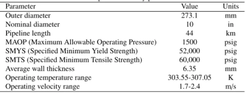
The case study evaluates a real carbon steel pipeline grade API5LX52 alloy; the pipeline characteristics are shown in Table 3. Two corrosion data sets were obtained from ILI measure-ments 2 years apart. In the first run, 33,466 defects were identified and in the second 59,101. For confidential agreements, further information about the case study cannot be provided.
Table 3: Pipeline summary parameters
Parameter Value Units
Outer diameter 273.1 mm
Nominal diameter 10 in
Pipeline length 44 km
MAOP (Maximum Allowable Operating Pressure) 1500 psig SMYS (Specified Minimum Yield Strength) 52,000 psig SMTS (Specified Minimum Tensile Strength) 60,000 psig
Average wall thickness 6.35 mm
Operating temperature range 303.55-307.05 K
Operating velocity range 1.7-2.4 m/s
Besides the information provided in Table 3, the distribution of the metal loss anomaly classi-fication on the inner and outer walls was determined following the criteria defined by the Pipeline Operators Forum [25]. It was obtained that: (i) almost 50% of the defects are classified as pit-ting, and the remaining are distributed mainly in circumferential slotpit-ting, and (ii) the metal loss defects are mostly located in the inner wall with around 80% in both ILI measurements. 5.2. Data treatment
Changes in the depth of defects were assessed based on observations of the two ILI mea-surements, and the defects were treated independently. Besides, since the exact type of the MFL tool used for pipeline inspection was not known; then, an uncertainty of 5 in the circumferential location of the defects during the inspection was assumed based on the vendor reports as it was described in Amaya-G´omez et al. [5]. This uncertainty corresponds to 12 mm or a deviation of 5%, obtaining two di↵erent data sets: (i) defects with a depth change between the two ILI measurements located in the same position; and (ii) defects with location di↵erences between the ILI measurements with a deviation less or equal to 5%. These sets are denoted as Set-1 and Set-2, respectively. Only defects with a correspondence between the two ILI measurements were taken into account; defects generated in the second inspection and those repaired have not been considered for this work
6. Results and discussion 6.1. Corrosion degradation model
Based on the two ILI inspections, depth-increments Xtwere computed (Eq. 9) for both Set-1
and Set-2. Moreover, the GP parameters from both sets were determined using the equations reported in Table 2 for t = 2 and with µ2,Xt =Var[Xt]):
g=(E[Xt]) 2 µ2,Xt· t g=E[Xt] µ2,Xt (12) The results are shown in Table 4. Despite the similarities between both sets, Set-2 includes depth-increments from Set-1. Considering the stationary assumption and a mean wall thickness of 6.35mm, the MTTF can be approximated linearly to 35.86 and 40.32 years for 1 and Set-2, respectively. Since this expected lifetime depends on the central moments of the degradation process [24], the MTTF obtained is conservative.
Table 4: GP Set-1 and Set-2 parameters
Set E[Xt]/t µ2,Xt/t g g
Set-1 0.1771 0.0325 0.9648 5.4477 Set-2 0.1575 0.0384 0.6456 4.0987
The Feasible Moments Criteria was implemented to select the degradation process that better describes the corrosion depth-increments using the second and third central moment [24]. The results indicate that a Mixed-L´evy Process with a GP as a progressive process and a shock-based process with shocks distributed as Delta-Dirac or Exponential should be considered. The corresponding mean and central moments for both distributions following the reported in Table 2 are [24]:
E[Wt] = ty, E[Wt]EXP= ty
Var[Wt] = ty2, Var[Wt]EXP=2 ty2
µ(3,Wt)| = ty3, µ(3,Wt)|EXP=6 ty3.
(13)
6.1.1. Optimization approach
Considering that the Set-1 is a subset of Set-2, the progressive degradation Zt parameters
were determined from the GP of the Set-1. Moreover, the mean and central moments from the ILI measurements were implemented in the proposed optimization process in Eq. 10. This equa-tion was solved using the Matlab ®Pattern Search algorithm, obtaining the optimum parameters shown in Table 5. These parameters indicate that the GP contributes the most to the degradation process. Although the inter-arrival time rates between shocks are almost the same between both mixed processes, there is a significant di↵erence between shock sizes.
Furthermore, the error obtained from the third central moment (µ3ILI) is almost 0 for the
Mixed GP+CPP- and GP+CPP-Exp processes (i.e., 1.4 · 10 10% and 7.4 · 10 11% respectively).
In both cases, the result was lower than 5.09% from GPS et2.
The pdf of the degradation distribution obtained using di↵erent models is presented in Fig.5 and it was compared with the data obtained from the ILI measurements. Although there are some discrepancies at lower corrosion values, in the tail of the distribution there is a good agreement between ILI data and the GPS et2and both Mixed processes. The mean degradation (and
coef-ficient of variation) for all models for t = 2 were: 0.3542 mm (0.720) for GPS et1, 0.3151 mm
Table 5: Mixed process parameters by optimization
Mixed process ↵p ↵s y
GP-CPP (Delta) 0.774 0.071 0.447 0.648 GP-CPP (EXP) 0.616 0.569 0.448 0.190
(0.881) for GPS et2, 0.3151 mm (0.881) for GP-CPP- , and 0.3152 mm (0.883) for GP-CPP-Exp.
The results from the mixed processes and the GPS et2 were closer to the obtained from the ILI
Data: 0.3150 mm (0.902). 0.1 0.2 0.3 0.4 0.5 0.6 0.7 0.8 0.9 1 0 0.5 1 1.5 2 2.5 3
Corroded wall thickness (mm)
pdf GPSet2 + CPP− δ ILI Data GPSet1 + CPP−Exp GPSet1 GPSet1
Figure 5: Corroded wall thickness probability density function.
6.2. Pipeline integrity assessment
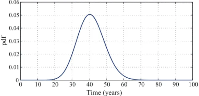
Based on a numerical approach, the corresponding reliability quantities were determined [24]. The expected corroded depth-increment was 0.15mm/year and the MTTF of 41.08 years, which is consistent to the mean lifespan of a pipeline (i.e., near 35 years) and the mean degrada-tion obtained in Amaya-G´omez et al. [5] for a plastic strain. In addidegrada-tion, the lifetime distribudegrada-tion for an intact pipeline in the Mixed Process is depicted in Fig. 6. Hereafter, the mixed process GP+CPP- is used to evaluate the pipeline integrity.
0 10 20 30 40 50 60 70 80 90 100 0 0.01 0.02 0.03 0.04 0.05 0.06 Time (years) pdf
Figure 6: Lifetime distribution for the Mixed Process.
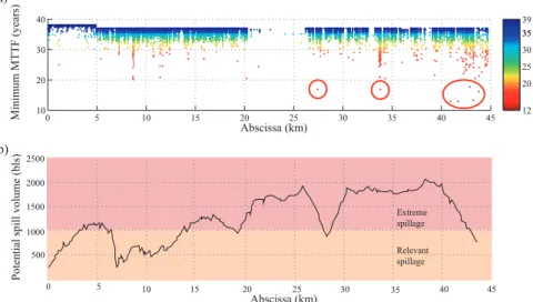
Assume that the pipeline is divided into equally spaced segments 1 m long each. The min-imum MTTF over the entire clock position can be calculated using the GP+CPP- model for every segment. In this particular case study, three leak-prone sections were identified; they are
located at: (i) km-27+4, (ii) km-33+7 and (iii) km-40+9; being the latter, the most critical with an approximately MTTF of 12 years once the evaluation was addressed in the last ILI inspec-tion. Besides, there is a pipeline segment around 43 km that has also reduced wall thickness. These sections were further studied in detail to provide a better insight into their criticality as it is shown in Fig. 7 using their potential spill volume. The results indicate that the these sections may produce extreme spillages in case of a LOC (i.e., over 1000 bls) by assuming a pump stop time of 5 minutes and considering the static volume and the pipeline altimetry. Note that the there are defects located near the 8th kilometer with a MTTF close to 20 years with potential spills under 500 bls, so these segments could be maintained after the three leak-prone sections aforementioned. The location of critical segments is important, but also the extent and type of defects. For example, once critical sectors are identified, possible interactions among the various defects within the segment could be evaluated.
0 5 10 15 20 25 30 35 40 45 10 20 30 40 Abscissa (km) M ini m um M T T F (ye ars ) 12 20 25 30 35 35 39 0 5 10 15 20 25 30 35 40 45 500 1000 1500 Abscissa (km) P ot ent ia l s pi ll vol um e (bl s) b) a) Extreme spillage Relevant spillage 2000 2500
Figure 7: a) Minimum MTTF and b) potential spill volume results along abscissa.
6.3. Maintenance program
In this example, the inspection, excavation, repair, and replacement unit costs are typical values of the industry in Canada reported in Zhang & Zhou [7], which represents a maintenance cost of C1 =80, 000 USD/Joint. For illustrative purposes, the replacement cost C2was selected
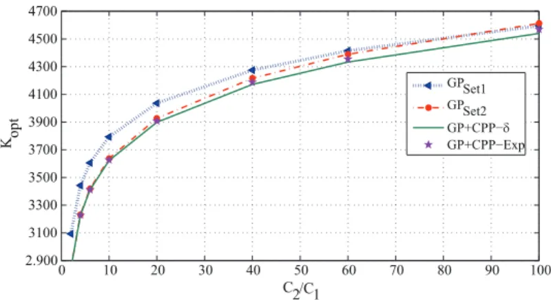
from the following C2/C1 ratios: 2, 4, 6, 10, 20, 40, 60, and 100. Based on the numerical
solution proposed in [42], the optimal replacement time was calculated for the four degradation processes discussed above; i.e., GPS et1, GPS et2, GPS et1+CPP and GPS et1+CPP-Exp (See
Fig. 8). A clear dependence between this optimal age of replacement with the failure cost C2
can be detected; namely, numerous inspections are required to avoid a costly failure. Besides, this figure shows that the results from the mixed processes and the GPS et2are almost the same,
whereas lower ages of replacement are expected for the GPS et1. This di↵erence seems to be
negligible, but let focus now on the expected cost rate.
Based on the optimal ages of replacement and Eq. 11, the expected cost rate for each degrada-tion process was determined and depicted in Fig. 9. Note that there is a di↵erence of at most 200
0 10 20 30 40 50 60 70 80 90 100 18 20 22 24 26 28 30 32 34 C 2/C1 αopt GPSet1 GPSet2 GP+CPP−δ GP+CPP−Exp
Figure 8: Optimal replacement ages in years vs C2/C1.
USD/Joint between the GPS et1 with the other degradation processes and an average di↵erence
of 50 USD/Joint between the Mixed Processes with the GPS et2. Considering that a pipeline may
have more than 3,000 joints, this di↵erence would represent an increase near 600,000 USD for the GPS et1and 150,000 USD for the GPS et2. Therefore, this di↵erence is nothing but negligible
and it illustrates how difficult is a maintenance decision-making process. Note that although the expected cost rates for the mixed processes are slightly shorter than the GPS et2, their optimal ages
of replacement are almost the same. The proposed approach can be used to support intervention decisions aiming to reduce investments in pipeline interventions and possible failures.
0 10 20 30 40 50 60 70 80 90 100 2.900 3100 3300 3500 3700 3900 4100 4300 4500 4700 C2/C1 Kopt GPSet1 GPSet2 GP+CPP−δ GP+CPP−Exp
Figure 9: Optimal cost in USD per unit time.
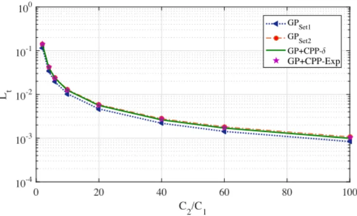
For instance, the cumulative failure distribution can be estimated up to each of the optimal ages of replacement not only to describe the decision following a cost-based approach but also to consider the probability of a future loss of containment on the pipe. Fig. 10 presents this estimation from the illustrative example, where a clear decreasing performance is depicted, once the failure or corrective cost growths. This tendency is expected because the optimal age of re-placement is reduced, so more frequent intervention takes place. However, this figure provides additional information about possible optimal ages that fit a similar ALARP (As Low As Reason-ably Practicable) perspective. Although the cost of failure increases significantly, in comparison
to the maintenance cost, the failure probability yields an almost stable point, regardless inspec-tions are implemented reiteratively when C2/C1>20. Depending on the company maintenance
policy, these results are useful to improve maintenance planning.
0 20 40 60 80 100 C2/C1 10-4 10-3 10-2 10-1 100 Lt GPSet1 GPSet2 GP+CPP-δ GP+CPP-Exp
Figure 10: Cumulative failure distribution until ↵opt.
7. Conclusions
A stochastic characterization of a corroded pipeline is presented in this paper based on a ILI (In-Line) inspections of a real pipeline using a Mixed L´evy Process composed by a Gamma and a Compound Poisson Processes. An optimization approach was proposed to estimate the parameters of this mixed process considering location uncertainties and a significant amount of detected defects. The results from the degradation process were then implemented in an integrity assessment based on the Mean Time to Failure (MTTF) along the pipeline and a maintenance approach following an Age of replacement model.
This characterization aims to fit the mean and central moments of the reported degradation. The results produced relevant di↵erences with a simple Gamma Process (GPS et2) in the optimal
replacement ages, which in turn, correspond to an increase about 150,000 USD in the expected cost rate for a pipeline with 3,000 joints. Regarding the integrity assessment, the MTTF helped identifying leak-prone segments of the pipeline, which in turn, were compared with the potential spill volume to recognize critical locations. These assessments seek to support a decision-making process regarding a pipeline intervention plan.
The proposed approach is a complementary alternative for codes/standards such as API 579-1/ASME FFS-1 for corroded pipeline assessments. A stochastic approach allows decision makers to obtain results that capture the underlying uncertainties of the complex degradation model.
Acknowledgments
R. Amaya-G´omez thanks the National Department of Science, Technology and Innovation of Colombia for the PhD scholarship (COLCIENCIAS Grant No. 727, 2015) and Campus France for the Ei↵el Excellence Program (2018).
Bibliography
[1] CONCAWE, Performance of European cross-country oil pipelines. Statistical summary of reported spillages in 2012 and since 1971, Tech. rep., Conservation of Clean Air and Water in Europe, online; accessed February 2015 (2013).
[2] US DoT PHMSA, Data and Statistics, http://www.phmsa.dot.gov/pipeline/library/data-stats, on-line; accessed February 2015 (2015).
[3] P. Tang, J. Yang, J. Zheng, I. Wong, S. He, J. Ye, G. Ou, Failure analysis and prediction of pipes due to the interaction between multiphase flow and structure, Engineering Failure Analysis 16 (5) (2009) 1749 – 1756. doi:http://dx.doi.org/10.1016/j.engfailanal.2009.01.002.
[4] G. Zhang, L. Zeng, H. Huang, X. Guo, A study of flow accelerated corrosion at elbow of carbon steel pipeline by array electrode and computational fluid dynamics simulation, Corrosion Science 77 (2013) 334 – 341. doi:http://dx.doi.org/10.1016/j.corsci.2013.08.022.
[5] R. Amaya-G´omez, M. S´anchez-Silva, F. Mu˜noz, Pattern recognition techniques implementation on data from In-Line Inspection (ILI), Journal of Loss Prevention in the Process Industries 44 (2016) 735 – 747. doi:http://dx.doi.org/10.1016/j.jlp.2016.07.020.
[6] M. Pandey, D. Lu, Estimation of parameters of degradation growth rate distribution from noisy measurement data, Structural Safety 43 (2013) 60 – 69. doi:http://dx.doi.org/10.1016/j.strusafe.2013.02.002.
[7] S. Zhang, W. Zhou, Cost-based optimal maintenance decisions for corroding natural gas pipelines based on stochastic degradation models, Engineering Structures 74 (2014) 74 – 85. doi:http://dx.doi.org/10.1016/j.engstruct.2014.05.018.
[8] F. Baz´an, A. Beck, Stochastic process corrosion growth models for pipeline reliability, Corrosion Science 74 (2013) 50 – 58. doi:http://dx.doi.org/10.1016/j.corsci.2013.04.011.
[9] S. Li, S. Yu, H. Zeng, J. Li, R. Liang, Predicting corrosion remaining life of underground pipelines with a mechanically-based probabilistic model, Journal of Petroleum Science and Engineering 65 (34) (2009) 162 – 166. doi:http://dx.doi.org/10.1016/j.petrol.2008.12.023.
[10] F. Caleyo, J. Vel´azquez, A. Valor, J. Hallen, Probability distribution of pitting corrosion depth and rate in underground pipelines: A Monte Carlo study, Corrosion Science 51 (9) (2009) 1925 – 1934. doi:http://dx.doi.org/10.1016/j.corsci.2009.05.019.
[11] NORSOK, CO2 corrosion rate calculation model, Tech. rep., Oslo, Norway (1998).
[12] C. de Waard, U. Lotz, Prediction of CO2 corrosion of carbon steel, in: NACE International, Houston, United States, 1993.
[13] NACE International, RP0502-2002 Pipeline External Corrosion Direct Assessment Methodology. Standard Rec-ommended Practice, Tech. rep., Houston,USA (2002).
[14] A. Barbian, M. Beller, In-Line Inspection of High Pressure Transmission Pipelines: State-of-the-Art and Future Trends, in: 18th World Conference on Nondestructive Testing, Durban, South Africa, 2012.
[15] Y. Sahraoui, R. Khelif, A. Chateauneuf, Maintenance planning under imperfect inspections of corroded pipelines, International Journal of Pressure Vessels and Piping 104 (2013) 76 – 82. doi:http://dx.doi.org/10.1016/j.ijpvp.2013.01.009.
[16] W. Gomes, A. Beck, Optimal inspection and design of onshore pipelines under external corrosion process, Struc-tural Safety 47 (2014) 48 – 58. doi:http://dx.doi.org/10.1016/j.strusafe.2013.11.001.
[17] C. Ossai, B. Boswell, I. Davies, Stochastic modelling of perfect inspection and repair actions for leak-failure prone internal corroded pipelines, Engineering Failure Analysis 60 (2016) 40 – 56. doi:http://dx.doi.org/10.1016/j.engfailanal.2015.11.030.
[18] H. Hong, Inspection and maintenance planning of pipeline under external corrosion considering generation of new defects, Structural Safety 21 (3) (1999) 203 – 222. doi:http://dx.doi.org/10.1016/S0167-4730(99)00016-8. [19] F. Caleyo, J. Vel´azquez, A. Valor, J. Hallen, Markov chain modelling of pitting corrosion in underground pipelines,
Corrosion Science 51 (9) (2009) 2197 – 2207. doi:http://dx.doi.org/10.1016/j.corsci.2009.06.014.
[20] W. Zhou, H. Hong, S. Zhang, Impact of dependent stochastic defect growth on system reliability of corroding pipelines, International Journal of Pressure Vessels and Piping 96 and 97 (2012) 68 – 77. doi:http://dx.doi.org/10.1016/j.ijpvp.2012.06.005.
[21] R. Nicolai, R. Dekker, J. van Noortwijk, A comparison of models for measurable deterioration: An application to coatings on steel structures, Reliability Engineering & System Safety 92 (12) (2007) 1635 – 1650, special Issue on {ESREL} 2005. doi:http://dx.doi.org/10.1016/j.ress.2006.09.021.
[22] D. Frangopol, M.-J. Kallen, J. van Noortwijk, Probabilistic models for life-cycle performance of deteriorating structures: review and future directions, Progress in Structural Engineering and Materials 6 (4) (2004) 197–212. doi:10.1002/pse.180.
[23] M. Abdel-Hameed, L´evy Processes and Their Applications in Reliability and Storage, Springer-Verlag Berlin Hei-delberg, 2014. doi:10.1007/978-3-642-40075-9.
[24] J. Riascos-Ochoa, M. S´anchez-Silva, G.-A. Klutke, Modeling and reliability analysis of systems subject to mul-tiple sources of degradation based on L´evy processes, Probabilistic Engineering Mechanics 45 (2016) 164 – 176. doi:http://dx.doi.org/10.1016/j.probengmech.2016.05.002.
[25] POF, Specifications and requirements for intelligent pig inspection of pipelines, Tech. rep., Pipeline Operators Forum (2008).
[26] B. Eiber, Overview of Integrity Assessment Methods for Pipelines, Tech. rep., Robert J. Eiber Consultant Inc (2003).
URL http://mrsc.org/getmedia/8B8FF358-4055-4D0E-9ED6-08AE41DA68B7/EiberOverview.aspx [27] K. Reber, M. Beller, Ultrasonic in-line inspection tools to inspect older pipelines for cracks in girth and long-seam
welds, in: Pigging and service association seminar, Aberdeen, Scotland, 2003.
[28] M. Pandey, Probabilistic models for condition assessment of oil and gas pipelines, NDT & E International 31. [29] S. Kuniewski, J. van der Weide, J. van Noortwijk, Sampling inspection for the evaluation of
time-dependent reliability of deteriorating systems under imperfect defect detection, Reliability Engineering & Sys-tem Safety 94 (9) (2009) 1480 – 1490, eSREL 2007, the 18th European Safety and Reliability Conference. doi:https://doi.org/10.1016/j.ress.2008.11.013.
[30] H. Qin, Probabilistic Modeling and Bayesian Inference of Metal-Loss Corrosion with Application in Reliability Analysis for Energy Pipelines, Master’s thesis, electronic Thesis and Dissertation Repository. Paper 2246. (2014). [31] S. Zhang, W. Zhou, H. Qin, Inverse Gaussian process-based corrosion growth model for energy
pipelines considering the sizing error in inspection data, Corrosion Science 73 (2013) 309 – 320. doi:http://dx.doi.org/10.1016/j.corsci.2013.04.020.
[32] M. S´anchez-Silva, G.-A. Klutke, Reliability and life-cycle analysis of deteriorating systems, Springer series in Reliability Engineering, Springer, 2016.
[33] M. S´anchez-Silva, G. Klutke, D. Rosowsky, Life-cycle performance of structures subject to multiple deterioration mechanisms, Structural Safety 33 (3) (2011) 206 – 217. doi:http://dx.doi.org/10.1016/j.strusafe.2011.03.003. [34] H. Qin, W. Zhou, S. Zhang, Bayesian inferences of generation and growth of corrosion defects on energy
pipelines based on imperfect inspection data, Reliability Engineering & System Safety 144 (2015) 334 – 342. doi:http://dx.doi.org/10.1016/j.ress.2015.08.007.
[35] S. Zhang, W. Zhou, System reliability of corroding pipelines considering stochastic process-based models for defect growth and internal pressure, International Journal of Pressure Vessels and Piping 111-112 (2013) 120 – 130. doi:http://dx.doi.org/10.1016/j.ijpvp.2013.06.002.
[36] J. van Noortwijk, A survey of the application of gamma processes in maintenance, Reliabil-ity Engineering & System Safety 94 (1) (2009) 2 – 21, maintenance Modeling and Application. doi:http://dx.doi.org/10.1016/j.ress.2007.03.019.
[37] J. van Noortwijk, M. Pandey, A stochastic deterioration process for time-dependent reliability analysis, in: Eleventh IFIP WG 7.5 Working Conference on Reliability and Optimization of Structural Systems, Ban↵, Canada, 2004. [38] N. Chen, Z.-S. Ye, Y. Xiang, L. Zhang, Condition-based maintenance using the inverse
Gaus-sian degradation model, European Journal of Operational Research 243 (1) (2015) 190 – 199. doi:https://doi.org/10.1016/j.ejor.2014.11.029.
[39] H. Qin, S. Zhang, W. Zhou, Inverse Gaussian process-based corrosion growth modeling and its application in the reliability analysis for energy pipelines, Frontiers of Structural and Civil Engineering 7 (3) (2013) 276–287. doi:10.1007/s11709-013-0207-9.
[40] W. Zhou, W. Xiang, H. Hong, Sensitivity of system reliability of corroding pipelines to modeling of stochas-tic growth of corrosion defects, Reliability Engineering & System Safety 167 (2017) 428 – 438, spe-cial Section: Applications of Probabilistic Graphical Models in Dependability, Diagnosis and Prognosis. doi:http://dx.doi.org/10.1016/j.ress.2017.06.025.
[41] W. Peng, Y.-F. Li, Y.-J. Yang, H.-Z. Huang, M. Zuo, Inverse Gaussian process models for degrada-tion analysis: A Bayesian perspective, Reliability Engineering & System Safety 130 (2014) 175 – 189. doi:https://doi.org/10.1016/j.ress.2014.06.005.
[42] J. Riascos-Ochoa, The L´evy-based framework for deterioration modeling, reliability estimation and maintenance of engineered systems, Ph.D. thesis, Universidad de los Andes, unpublished Thesis (2016).
[43] H. A. Kishawy, H. A. Gabbar, Review of pipeline integrity management practices, International Journal of Pressure Vessels and Piping 87 (7) (2010) 373 – 380. doi:http://dx.doi.org/10.1016/j.ijpvp.2010.04.003.
[44] R. Amaya-G´omez, M. S´anchez-Silva, E. BastidArteaga, F. Schoefs, F. Mu noz, Reliability as-sessments of corroded pipelines based on internal pressure A review, Engineering Failure Analysis-doi:https://doi.org/10.1016/j.engfailanal.2019.01.064.
[45] J. Fontecha, N. Cano, N. Velasco, F. Mu noz, Optimal sectioning of hydrocarbon transport pipeline by volume min-imization, environmental and social vulnerability assessment, Journal of Loss Prevention in the Process Industries 44 (2016) 681 – 689. doi:https://doi.org/10.1016/j.jlp.2016.07.017.
Appendix A. Estimation of degradation parameters GP and IGP processes
The parameters of the gamma distribution can be determined using the method of moments described in [37]. This method uses the mean and variance of the degradation process, to de-termine the c parameter from the shape function v(t) = ctband the constant scale parameter u.
If the power b is known, this non-stationary GP can be transformed into a stationary degrada-tion process by the map z = tb. Otherwise, this parameter could be determined numerically by
the method of Maximum Likelihood [21]. As a result of the method of moments, the estimate of these parameters (i.e., ˆc and ˆu) can be obtained using the time between inspections wj=(tj tj 1),
the degradation of each defect xi
j, and defect-depth increments ij=(xij xij 1) with t0=0 [37]:
ˆc ˆu = Pn j=1 ij Pn j=1wj = x i n tn := ¯i, xi n ˆu 0 BBBBB BBB@1 Pn j=1w2j hPn j=1wj i2 1 CCCCC CCCA = n X j=1 ⇣ i j ¯iwj⌘2 (A.1)
Moreover, in a reliability-based pipeline integrity assessment it is common to assume a linear growth of the corrosion rate (i.e., b = 1) because of its simplicity [20]. Considering that pipeline inspections are carried out periodically every 2 to 4 years, these expressions can be simplified using a constant inspection interval ⌧ as follows:
ˆc ˆu = ¯i, xi n ˆu 1 1 n ! =n⌧2¯2i 2¯i⌧xin+ n X j=1 ⇣ i j ⌘2 (A.2)
In case only two ILI inspections are considered in an homogeneous case (i.e., b = 1), this procedure is simplified as follows:
c = E[Xt]2
t · Var[Xt], u = E
[Xt]
Var[Xt] (A.3)
Similar results can be obtained for the IGP process, which variance and coefficient of varia-tion are given as follow:
Var[Xt] = ⇤t
⇣ , COV[Xt] = 1 p
⇣⇤t
In this case, the parameters ⇤t= ⇤0t and ⇣ are given by:
⇤0=E[Xt]
t , ⇣ = E[Xt]
Var[Xt] (A.4)
The mean and the variance of both stochastic processes are summarized in Table A.6.
Table A.6: GP and IGP mean and variance [31, 36]
Process Mean Variance
GP E[Xt] =v(t)u Var[Xt] =v(t)u2 IGP E[Xt] = ⇤t Var[Xt] =⇤t
![Figure 1: Scheme of the location of a corrosion defect. Modified from [25].](https://thumb-eu.123doks.com/thumbv2/123doknet/11322917.282891/4.892.166.734.431.595/figure-scheme-location-corrosion-defect-modified.webp)
![Table 1: Resolution of measurement parameters [25].](https://thumb-eu.123doks.com/thumbv2/123doknet/11322917.282891/5.892.284.607.454.573/table-resolution-of-measurement-parameters.webp)
![Figure 4: Age-Replacement Model representation. Modified from [32].](https://thumb-eu.123doks.com/thumbv2/123doknet/11322917.282891/12.892.297.596.695.827/figure-age-replacement-model-representation-modified-from.webp)