1
Predicting the age of researchers using
bibliometric data
Gabriela F. Nane
a,1, Vincent Larivière
band Rodrigo Costas
c aDelft Institute of Applied Mathematics, Delft University of Technology, The Netherlands
b
Centre Interuniversitaire de Recherche sur la Science et la Technologie (CIRST), Université du Québec à Montréal, Canada
c
Center for Science and Technology (CWTS), Leiden University, The Netherlands
Abstract
The age of researchers is a critical factor necessary to study the bibliometric characteristics of the scholars that produce new knowledge. In bibliometric studies, the age of scientific authors is
generally missing; however, the year of the first publication is frequently considered as a proxy of the age of researchers. In this article, we investigate what are the most important bibibliometric factors that can be used to predict the age of researchers (birth and PhD age). Using a dataset of 3574 researchers from Québec for whom their Web of Science publications, year of birth and year of their PhD are known, our analysis falls under the linear regression setting and focuses on investigating the predictive power of various regression models rather than data fitting, considering also a breakdown by fields. The year of first publication proves to be the best linear predictor for the age of
researchers. When using simple linear regression models, predicting birth and PhD years result in an error of about 3.7 years and 3.9 years, respectively. Including other bibliometric data marginally improves the predictive power of the regression models. A validation analysis for the field
breakdown shows that the average length of the prediction intervals vary from 2.5 years for Basic Medical Sciences (for birth years) up to almost 10 years for Education (for PhD years). The average models perform significantly better than the models using individual observations. Nonetheless, the high variability of data and the uncertainty inherited by the models advice to caution when using linear regression models for predicting the age of researchers.
Introduction
Several sociodemographic factors have been shown to affect researchers’ scholarly output and impact (Costas & Bordons, 2011; Gingras, Larivière, Macaluso, Robitaille, 2008; Mauleón & Bordons, 2006). Among those, we can mention age (Costas & Bordons, 2011; Gingras et al., 2008; Levin & Stephan, 1989), gender (Larivière, Gingras, Cronin, & Sugimoto, 2013; Mauleón & Bordons, 2006), mobility and migration (Canibano, Otamendy, & Solis, 2011; Franzoni, Scellato, & Stephan, 2012; Moed & Halevi, 2014).
The development of large scale author-name disambiguation algorithms (Caron & Van Eck, 2014), as well as the increasing quantity of indexed papers’ metadata (e.g. author names and surnames, affiliations, e-mail data, etc.) have expanded the possibilities to study such sociodemographic variables . For example, the analysis of the first author names of authors (Larivière et al., 2013)
1 Corresponding author. E-mail address: [email protected].
2
allowed for the macro analysis of gender disparities worldwide. The large-scale analysis of the relationship between author names, affiliations and countries has also opened the possibility of studying academic migrations at the world level (Moed, Aisati, & Plume, 2013), as well as the nationality (Costas & Noyons, 2013) or even the ethnic origin (Freeman, 2014) of scholars.
One of the central sociodemographic characteristics of scholars is their age (Costas & Bordons, 2011; Gingras et al., 2008; Levin & Stephan, 1989), as it has been shown to be a key predictor of research productivity (Bornmann & Leydesdorff, 2014; Falagas, Ierodiakonou, & Alexiou, 2008; Levin & Stephan, 1989). However, such variable is generally not included in bibliometric analyses, given its lack of availability. While several analyses have used the year of first publication as a proxy for their age, of a scholar (e.g. Radicchi & Castellano, 2013), there has not been any analysis on the actual relationship between this proxy and the real age of scholars. This paper is intended to fill this gap and shed some light on the underlying relationship between the ‘bibliometric’ age of scholars and their ‘real’ ages, defined as their biological age and time to PhD. In other words, we aim to assess how reliable is the estimation of the real ages of scholars based on models that exclusively rely on bibliometric indicators, such as the year of first publication, author order, co-authors, document types published, etc.).
Firstly, we will investigate the correlations between all the variables considered in the analysis. Furthermore, several boxplots of the birth and PhD year will be presented and analysed in order to study the dispersion of the actual data. The next step in our analysis will focus on linear regression model fitting2. Therefore the birth (BIRTH hereafter) and PhD (PHD hereafter) years will be most
frequently referred to as the ‘dependent variables’, while the bibliometric variables will be interchangeably referred to as the ‘independent variables’, covariates or predictors.
Methodology
For the study proposed it is absolutely necessary to have a dataset of scholars for whom the real ages of all the individuals considered are certainly known as well, as the publication years of their
scientific publications, conforming the ‘golden set’ of the study. As golden set we have considered one of the (possibly) largest datasets of individual scholars for whom their actual individual characteristics are known (this dataset has been used in some previous studies, e.g. Gingras et al., 2008; Larivière et al., 2011). The dataset is composed by 13,626 university professors from Quebec (Canada) who have published at least one article indexed in the Web of Science (WoS) database during the 1980-2012 period. For every scholar in the dataset, different information has been collected, including their biological (BIRTH) and academic (PHD) ages, along with other bibliometric data, such as the year of first publication (YFP), number of publications in WoS (P), the proportion of publications with the scholar in the first position (PP_POS_FIRST), the proportion of publications with any type of international collaboration (PP_INT_COLLAB), etc. The full list of variables considered can be found in Table A1 of the Appendix.
The data also include information about the research domain of the scholars. A total of nine disciplinary fields of activity of the scholars are considered, based on the 2000 revision of the U.S.
2 Despite its strong (and sometimes unintuitive) assumptions that are frequently violated in practice, linear
regression modelling remains nevertheless the typical (first) approach in investigating the relationships between the variables of interest and covariates.
3
Classification of Instructional Programs (CIP)3 developed by the U.S. Department of Education's National Center for Education Statistics (NCES). The nine fields of activity, as well as the distribution of researchers among the fields can be seen in Table A2 in the Appendix.
For the robustness of the results, we have selected researchers that are born after 1960 and have obtained their PhD degree since 1980. Moreover, since the last recorded PhD year is 2005, we have selected only the researchers that have their first publication the latest in 2010. Therefore the variable YFP is bounded at 2010 and the data truncated correspondingly.
Our final dataset comprises of 3,574 researchers. Using this sample, we will make inferences about the researchers, in general, who represent our statistical population. We believe our sample is representative for researchers, in general. The external validation of our analyses, using another dataset, will be deferred to another manuscript.
The subsequent analysis is divided in two main parts. Firstly, we will perform an ‘overall analysis’, for all the selected researchers in the dataset, regardless their field of activity. We employ linear
regression models for average birth and PhD years, as well as for all individual observations.
Secondly, we are also interested in the particular characteristics of researchers in different fields and examine the potential disciplinary differences in the results. We therefore apply a similar analysis at the field level.
Overall analysis
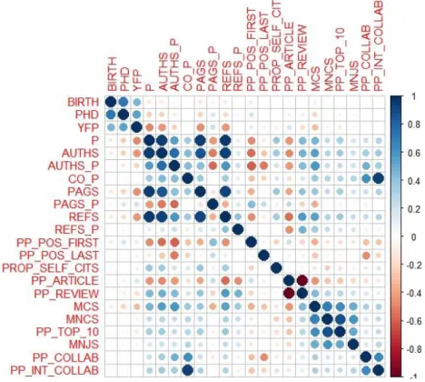
We start our analysis by investigating the Spearman rank correlation among all variables in the study (see Table A1 in the Appendix). The correlation matrix is depicted in Figure 1. The correlation plot illustrates the correlations between BIRTH and PHD with other variables, and also brings insight into the correlations between the different independent variables. The age-related variables are well correlated among themselves. That is, birth (BIRTH) and PhD year (PHD) of researchers exhibit a strong correlation. Moreover, the year of first publication (YFP) is the only independent variable that presents a substantial correlation with these two age-related variables. Figure 1 provides clear evidence to support the idea that YFP is the most relevant bibliometric variable for the estimation and potential prediction of the real age of scholars. The correlations between BIRTH and PHD with the other variables are very low and hence barely visible on the plot. Although small, the largest positive correlation is with the proportion of publications where the researcher has the first position in the author’s list (PP_POS_FIRST).
Some correlations observed in Figure 1 also reflect, at the researcher level, expected relationships between variables, such as the total number of publications (P) and the proportion of articles from the total output (PP_ARTICLE), the average number of countries per paper (CO_P) and the
percentage of publications resulting from international collaborations (PP_INT_COLLAB), or the correlation between the thee field-normalized size-independent impact indicators (MNCS,
PP_TOP_10 and MNJS). Also the collaboration indicators (e.g. number of countries per paper (CO_P), the proportion of collaborative publications (PP_COLLAB) and the proportion of publications in international collaboration (PP_INT_COLLAB) exhibit an expectedly strong correlation. Negative
3 The Classification of Instructional Programs (CIP) is developed by the U.S. Department of Education's
National Centre for Education Statistics (NCES). More details can be found at: http://nces.ed.gov/pubs2002/cip2000/
4
correlations emerge as well. For example, we note the negative correlation between the mean number authors per publication (AUTHS_P) and the proportion of publications where the researcher has been the first (PP_POS_FIRST) as well as the last author (PP_POS_LAST). It suggests co-authoring publications with higher number of authors, on average, reduces the likelihood of being the first or the last author.
Figure 1. Correlation plot of all variables in the analysis.
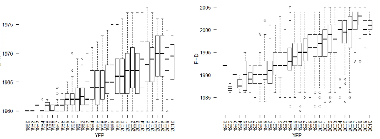
In Figure 2, we focus now on the relationship between YFP and BIRTH and PHD, presenting the boxplots of BIRTH and PHD against YFP. That is, for each distinct YFP, we consider the boxplot of BIRTH and PHD. Both distributions exhibit a large degree of variation (spread) for almost all years of first publication. The low spread in the lowest and highest YFP is mainly due to the low number of observations in those cases. This suggests that, despite general incremental patterns, there is also a significant dispersion in the data concerning the age of researchers. Notably, the spread and thus the variation of data increases with the year of first publication, especially for the BIRTH variable. The interquartile range however remains approximately constant over the YFP. This indicates that the central 50% of values within the BIRTH and PHD years grouped by YFP are similarly dispersed. With respect to outliers, we note more outliers for the PhD years.
5
Figure 2. Boxplot of birth year (left) and PhD year (right) over year of first publication (YFP).
Average model
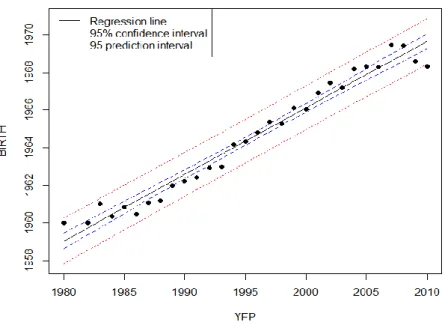
In this section we focus on linear regression modelling in order to predict the BIRTH and PHD ages of researches based on the YFP. Firstly, we consider an average model, that is for each distinct YFP we average the BIRTH and PHD variables for the researchers under analysis. Since our analysis contains 31 distinct YFP (1980-2010), the BIRTH and PHD models are fitted using 31 observations. The
regression line, as well as the confidence and prediction bounds are depicted in Figures 3 (for BIRTH) and 4 (for PHD). The dotted points represent the observed average BIRTH and PHD years. The confidence and prediction intervals are computed by using the standard error of the residuals (the difference between the observed and the fitted values). The confidence intervals account for the uncertainty in estimating the true BIRTH and PHD average years, whereas the prediction intervals account for the uncertainty inherited by a random future BIRTH or PHD year. Consequently, the prediction intervals are wider than the confidence intervals. Nonetheless, the prediction intervals are more appropriate for making statistical inference.
6
Figure 3. Simple average BIRTH model: the linear fit (black line), the confidence bounds (blue, dashed line), and the prediction bounds (red, dotted line). The black points denote the observations in the average model.
The two simple linear models display a remarkable fit for the data on average BIRTH and PHD years, indicating a strong linear relationship between average BIRTH and PHD with YFP and, moreover, that YPF is a very good linear predictor of average BIRTH and PHD years.
Figure 4. Simple average PHD model: the linear fit (black line), the confidence bounds (blue, dashed line), and the prediction bounds (red, dotted line). The black points denote the observations in the average model.
7
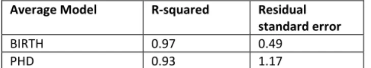
To quantify the goodness of fit, we explore some standard error measurements. Apart from R-squared, we report the residual standard error. The table below provides these statistics for the two models.
Average Model R-squared Residual
standard error
BIRTH 0.97 0.49
PHD 0.93 1.17
Table 1. R-squared, adjusted R-squared and residual standard error for the BIRTH and PHD average model.
Note the high values for R-squared4 in both average models. It can be concluded that 97% of the total variation is explained by the simple average BIRTH model, whereas 93% of the total variation is explained by the linear PHD model.
It is well known that, in general, R-squared does not necessarily indicate a good fit of the linear model. With this respect, we quantify the goodness of fit by using the residual standard error (Table 1). The residual standard error yields that the prediction of the average PhD year from the simple linear regression results, on average, in an error of about 1.2 years. For the average birth year, the error is about 0.5 years. Furthermore, if the residuals are approximately normal, then about 95% of the average birth years are in the range ±1 year (and the average PhD years are in the range ±2.4 years). The residuals of the BIRTH model look approximately normal (see Figure A1 in Appendix5). However, the residuals of the PHD model (see Figure A2 in Appendixes) exhibit a long tail, hence the departure from normality. It has to be born in mind though that the models are fitted using a small number of observations (31 observations).
So far we have focused on the averages of BIRTH and PHD years. However, it would be of high interest to investigate how well do the average models describe the entire dataset at the
observational level. That is, how well do the average models based on YFP predict the ages of the individual researchers in the analysis? We report (Table 2) the percentage of covered observations within the confidence and prediction intervals, as well as the average length (in years) of the confidence and prediction intervals.
Model Interval Coverage
Percentage (all)
Average length (years) Intervals Coverage Percentage (IQR) BIRTH Confidence 4.17% 0.51 7.11% Prediction 20.35% 2.11 34.58% PHD Confidence 11.3% 1.21 18.64% Prediction 46.25% 4.97 79.84%
Table 2. Coverage percentage and average length intervals (in years) of the average models confidence and prediction intervals for individual observations. The coverage percentages are reported for the entire dataset (all) and for the observations in the interquartile range (IQR).
Firstly, we observe higher coverage percentages and corresponding smaller average length intervals for BIRTH model than for PHD model. Based on that, the average PHD model seems to cover, via the confidence and prediction intervals, twice as many researchers as the BIRTH model. The average intervals are twice as small for the BIRTH model than for the PHD model. Differently put, it seems that the first publication year (YFP) is a better linear predictor (in the average model) for academic age than for biological age. Finally, we have investigated how well do confidence and prediction
4
For simple linear regression, R-squared is the squared Pearson correlation.
5
The density plots of the residuals, as well as the qqplots for the two average models can be found in Figures A1 and A2 in the Appendix.
8
intervals cover researchers within their specific interquantile range (IQR). The IQR are determined for each distinct year of first publication, as depicted in Figure 2. It is noteworthy that almost 80% of the observations within the IQR fall within the prediction intervals of the PHD average model.
Nevertheless, the other percentages of coverage of prediction and confidence intervals are quite low (with less than 50% of all individual observations), indicating that the bounds obtained from the average model should be used with care for single observations.
Model selection
The main conclusion of previous section is that, in general, the promising results obtained in the average simple models should not be carelessly transferred for individual researchers. In this section we investigate how well do linear regression models work, when performed at the level of individual researchers.
We will thus focus now on fitting linear regression models based on all observations (instead of averages). We will consider simple linear regression models, with YFP as the independent variable for both BIRTH and PHD dependent variables. Moreover, we will explore whether other independent variables could also predict the BIRTH and PHD variables. Thus, we will consider all the variables presented in Table A1 (in the Appendix) and employ model selection techniques to choose the most influential independent variables for the prediction of the dependent variables.
The standard procedure for the linear regression models is the stepwise regression selection (see, for example, Fox, 2008). The (stepwise) ‘forward’ selection starts with a model with no variables and adds at each step the independent variable that improves the model the most. The procedure terminates when no variable, if added, would improve the model. The (stepwise) ‘backward’ selection starts with the full model, when all independent variables are included and eliminates at each step the variable that, if deleted, would improve the model the most. The procedure is repeated until no improvement is possible. The stepwise ‘both’ procedure is a combination of the two previous methods, where, at each step, variables are either included or excluded in order to improve the model. The model improvement is measured with the Bayesian information criterion (BIC) and is indicated by low values of BIC. BIC is expressed in terms of the likelihood function of the model, as well as a penalty term that accounts for the number of independent variables and the number of observations. The penalty term precludes overfitting.
Selection model Dependent
variable
Independent Variables selected BIC
Stepwise forward
BIRTH
YFP, P, AUTHS, AUTHS_P, CO_P, PAGS, PAGS_P, REFS, REFS_P, PP_POS_FIRST, PP_POS_LAST, PROP_SELF_CITS, PP_ARTICLE, PP_REVIEW, MCS, MNCS, PP_TOP_10, MNJS, PP_COLLAB, PP_INT_COLLAB
18960
PHD
YFP, P, AUTHS, AUTHS_P, CO_P, PAGS, PAGS_P, REFS, REFS_P, PP_POS_FIRST, PP_POS_LAST, PROP_SELF_CITS, PP_ARTICLE, PP_REVIEW, MCS, MNCS, PP_TOP_10, MNJS, PP_COLLAB, PP_INT_COLLAB
19279.96
Stepwise backward
BIRTH YFP, PP_POS_LAST, PROP_SELF_CITS, PP_TOP_10 18864.3 PHD YFP, REFS_P, PP_POS_FIRST, PP_POS_LAST, PROP_SELF_CITS,
PP_ARTICLE, MCS, MNCS, PP_COLLAB, PP_INT_COLLAB
19212.38
Stepwise both
BIRTH YFP, PP_POS_LAST, PROP_SELF_CITS, PP_TOP_10 18864.3 PHD YFP, REFS_P, PP_POS_FIRST, PP_POS_LAST, PROP_SELF_CITS,
PP_ARTICLE, MCS, MNCS, PP_COLLAB, PP_INT_COLLAB
9
Table 3. Stepwise regression birth and PhD models using BIC criterion.
Using stepwise forward regression gives that all 20 independent variables enter the PHD and BIRTH models. When using stepwise backward selection, the BIRTH model includes only 4 independent variables. According to this procedure, the most influential variables for the biological age are YFP, proportion of publications where the researcher is on the last position (PP_POS_LAST), the
proportion of self-citations (PP_SELF_CITS), as well as PP_TOP_10. The PHD final model when using stepwise backward selection includes 10 independent variables. These variables include the predictors from the birth model, except PP_TOP_10, along with the references per publication (REFS_P), the proportion of publications that are articles (PP_ARTICLE), MCS and MNCS and the proportion of publications that were the result of (international) collaborations (PP_COLLAB and PP_INT_COLLAB). The lowest BIC values are registered for the stepwise backward selection,
indicating an improvement in the goodness-of-fit of the model by excluding 16 variables for the birth model and 10 variables for the PhD model. The results for stepwise backward and both selection coincide.
We have also considered models that account for interactions between the independent variables. However, the model included all the independent variables, along with 45 other interaction terms between the independent variables. The model does not perform better in terms of BIC, residual standard error or adjusted R-squared. For this reason, we chose not to report models including interactions and restrict only to full models (when including all the independent variables) and models resulted from stepwise selection using backward elimination.
Predictive power of the observation-based models. Considering all the previous models discussed, the question that arises now is, of course, which model can be considered the best in order to predict the real ages of researchers? In order to answer this question, in this section we evaluate the models obtained via the chosen methods from a predictive point of view.
In order to simplify the discussion, we consider the following BIRTH and PHD models: 1) ‘Full model’, containing all the 20 independent bibliometric variables;
2) ‘Simple model’, that is the model with YFP as its unique independent variable (predictor) 3) ‘Backward model’, this is the model based on the stepwise backward elimination.
We first analyse the models according to how well they describe the data, by reporting R-squared and adjusted R-squared, that corrects for the number of independent variables. The aim, however, is to quantify the predictive power of the three linear regression models. With this respect, we employ the predicted residual sum of squares (PRESS) statistics, also known as the P-square (Allen, 1974). The PRESS statistic performs cross-validation and the residual sum of squares is computed by fitting the model for a subset of all the observations (a sample). Then it is calculated if the model is
predicting well the observations out of the sample, thus considering the squares of all the prediction errors. The smaller the PRESS statistics, the higher the predictive power. Thus, checking the
predictive power of the model constitutes a validity check for the models as well. Results containing the R-squared, adjusted R-squared, Residual Standard Error and BIC and PRESS statistics are
10
Model R-squared Adjusted
R-squared
Residual Std. Error
BIC PRESS
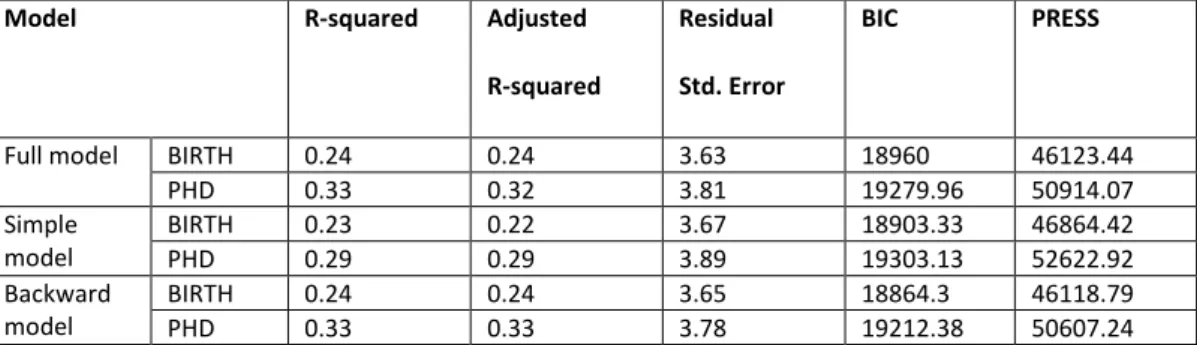
Full model BIRTH 0.24 0.24 3.63 18960 46123.44 PHD 0.33 0.32 3.81 19279.96 50914.07 Simple model BIRTH 0.23 0.22 3.67 18903.33 46864.42 PHD 0.29 0.29 3.89 19303.13 52622.92 Backward model BIRTH 0.24 0.24 3.65 18864.3 46118.79 PHD 0.33 0.33 3.78 19212.38 50607.24
Table 4. Goodness-of-fit statistics and predictive analysis for BIRTH and PHD proposed models.
For all our 6 models, the differences between R-squared and adjusted R-squared are small, indicating that correcting for the number of variables does not reduce the percentage of variation explained by the linear model. The differences between the R-squared values in all models is also small. Minor differences are noted for the residual standard errors as well. In comparison with average models (see Table 1), the results are modest, for all models.
In terms of predictive power, we observe that, in general, BIRTH models have higher predictive power (lower PRESS values) than the PHD models. The best predictive models are those resulted from performing stepwise backward regression. Therefore, reducing the number of variables from 20 to 4 in the BIRTH model and to 10 in the PHD model results in an increase in the predictive power. Even though the simple models have the lowest predictive power, the increase in predictive power of the other models is modest. Differently put, reducing the models to the simple linear regression (with YFP as the independent variable) results in a decrease of less than 2% in the predictive power for the BIRTH model and less than 4% for the PHD model.
To quantify the predictive error, we use the results of the residual standard error. Again, the
differences are very small between the three models. The lowest predictive error is observed for the models resulted from stepwise backward elimination and the full models. Predicting BIRTH years when using the simple linear regression model results in an error of about 3.7years, while predicting PHD years when using simple linear regression results in an error of about 3.9. This error is much higher than the error obtained for the simple average models, indicating that prediction errors significantly increase when considering individual observations. When comparing the backward model with the simple model, the decrease in the prediction error is 0.02 for the BIRTH models and 0. 09 for the PHD models, suggesting once more that adding more variables amounts in a slight reduction of the prediction error.
Validation of the simple linear models
The results obtained so far support the idea that YFP is the single best linear predictor of BIRTH and PHD ages of scholars. Accounting for other information marginally increases the performance of the linear models. To further validate this conclusion, in this section we investigate the performance of the simple linear regression models (based only on YFP) by splitting the dataset randomly in 2 dataset (A and B)6. Dataset A contains 2500 observations, whereas dataset B contains the remaining
970 observations. We fit the simple linear models on A and check how many observations in dataset B are covered by the confidence and prediction bounds obtained from fitting the model on the training set A. We also compute the average length for the confidence and prediction intervals. We
11
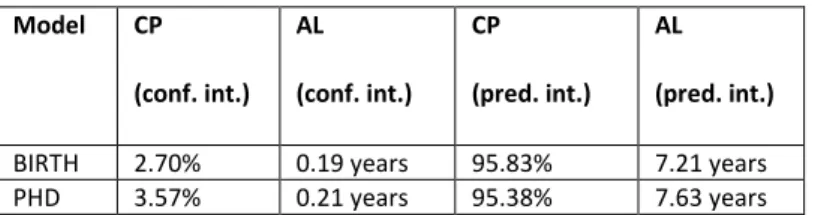
repeat this procedure 1000 times and average the obtained coverage percentages. The results are provided in Table 5. Model CP (conf. int.) AL (conf. int.) CP (pred. int.) AL (pred. int.)
BIRTH 2.70% 0.19 years 95.83% 7.21 years PHD 3.57% 0.21 years 95.38% 7.63 years
Table 5. Confidence and prediction average coverage percentages (CP) of observations in the test set (B) for 1000 runs for BIRTH and PHD models fitted on the training set (A). The average length (AL) of the confidence and prediction intervals.
The results indicate that the simple linear BIRTH and PhD models based on YFP can accurately predict, on average, more than 95% of researcher’s birth and PhD years. This coverage is achieved by the prediction intervals, that have, in turn, an average length of around 7 years for the BIRTH model and more than 7.5 years for the PHD model. The confidence intervals are very small, on average, of around 3 months, and therefore lead to poor coverage percentages. Despite the somewhat larger prediction intervals, the PHD years in the test dataset are slightly less covered. As mentioned beforehand, the high coverage percentages are due to the large prediction intervals, whereas the small confidence intervals lead to very small coverage percentages.
Field analysis
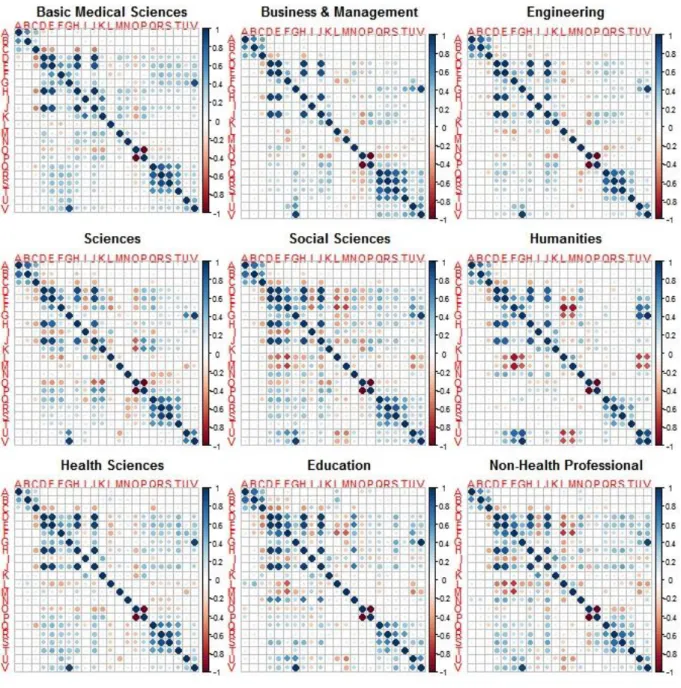
As mentioned before (see Methodology section), the researchers in our dataset are assigned to 9 fields (divisions). The fields, as well as the distribution of researchers over each field can be found in Table A2 in the Appendix. Most of the researchers are assigned to the “Sciences”, “Basic Medical Sciences” and “Engineering” fields. The correlation plots in Figure 5 depict graphically the differences in correlations among all 9 fields.
12
Figure 5. Correlation plots for all the fields in the analysis. The variables are denoted by letters (A to V), which can be found in Table A1. in the appendix.
Some of the obvious correlations previously observed in Figure 1 are also observed across fields. The most important similarity is that the correlation between the age variables (BIRTH and PHD) and YFP is high across all fields. An exception to the previously observed strong correlation between MNCS and PP_TOP_10 is that this is not observed in fields such as “Social Sciences”, “Humanities”,
“Education” and “Non-health professional”, which is likely a consequence of the lower applicability of citation analysis to those disciplines. Following the analysis for the entire dataset, Figure 6 depicts the distribution of BIRTH years over the YFP for all the fields in the analysis.
13
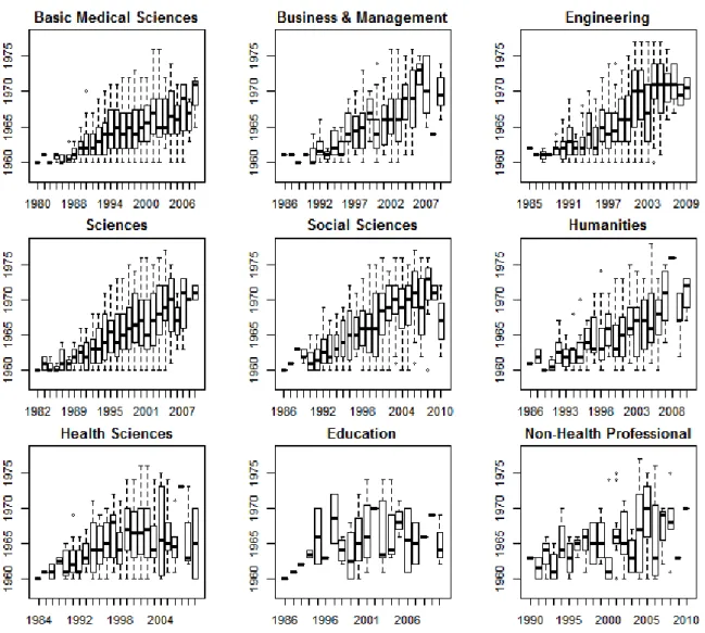
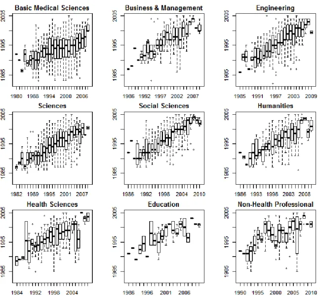
Figure 6. Boxplot of BIRTH vs. first publication year (YFP) for all fields.
In general, the boxplots for 7 of the 9 fields look quite similarly; showing a strong relationship BIRTH and YFP. The distortions in the boxplots for “Education” and “Non-health professional” are produced by the small number of observations in those fields. The variability of the data is evident for most of the fields via the whiskers of the boxplots. In “Basic Medical Sciences”, “Engineering” and “Sciences” especially, it is notable that researchers born in 1960 have their first publication as late as 2006.
14
Figure 7. Boxplot of year of first publication (YFP) vs. PHD for all fields.
Figure 7 presents the boxplots of PHD years with respect to YFP. Once again, all graphs have a quite similar pattern, with increasing trends in PhD years, although some fields seem to have more stable patterns (e.g. “Engineering”, “Sciences”, “Social Sciences” or “Health Sciences”), while others have more unstable patterns (e.g. “Non-Health Professional” and “Education”). The unstable patterns are mainly caused by the low number of observations in those fields.
Average model
For each distinct year of first publication and field, we can considered the average BIRTH and PHD years of researchers. The simple linear regression models have been fitted to the data and the resulting fit, along with confidence and prediction bounds are included in Figure 8.
15
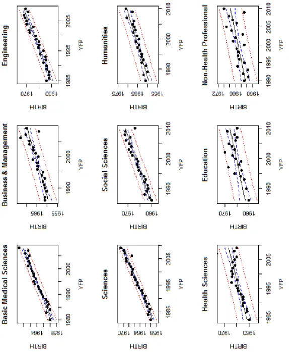
Figure 8. Simple average BIRTH models for all the fields: the linear fit (black line), the confidence bounds (blue, dashed line), and the prediction bounds (red, dotted line). The black points denote the observations in the average model.
All in all, the linear pattern is noticeable across all fields considered. The simple average BIRTH models exhibit a very good fit in “Basic Medical Sciences”, “Engineering”, “Sciences”, “Social
Sciences” and “Humanities”. Despite higher variations captured by larger confidence and prediction bounds, a linear pattern is also perceptible for “Business & Management”, as well as for “Health Sciences”. Only for “Education” and “Non-Health Professional”, the linear average model does not really fit the data very well. Once again, we should bear in mind the low number of observations used to fit the models.
16
Figure 9. Simple average PHD models for all the fields: the linear fit (black line), the confidence bounds (blue, dashed line) as well as the prediction bounds (red, dotted line). The black points denote the observations in the average model.
The graphical representation for the PHD simple average models for all fields is included in Figure 9. In general, patterns are comparable to the overall BIRTH average models. Similar as to the overall analysis, we compute the coverage percentages of the average BIRTH and PHD model for the individual researchers in the analysis, corresponding to each field. Results are provided only for the prediction intervals, in the table below.
Field (n. individuals) Model Coverage percentage (all) Average length of prediction interval Coverage percentage (IQR)
Basic Medical Sciences (713)
BIRTH 27.89% 2.56 47.56% PHD 52.82% 6.48 86.45% Business & Management
(238) BIRTH 72.46% 7.74 96.09% PHD 63.56% 6.41 91.11% Engineering (514) BIRTH 36.08% 4.07 59.57% PHD 48.63% 5.41 79.51% Sciences (824) BIRTH 24.48% 2.78 41.08% PHD 36.91% 3.92 59.75%
17 Field (n. individuals) Model Coverage percentage (all) Average length of prediction interval Coverage percentage (IQR) Social Sciences (500) BIRTH 48.27% 5.11 75.60% PHD 61.31% 6.03 90% Humanities (342) BIRTH 65.82% 7.69 90.41% PHD 58.18% 6.29 83.01% Health Sciences (288) BIRTH 63.54% 7.49 86.16% PHD 75.69% 8.27 96.91% Education (47) BIRTH 65.12% 7.71 82.61% PHD 95.34% 9.87 100% Non-Health Professional (108) BIRTH 65.63% 7.73 81.13% PHD 85.42% 9.29 96.36%
Table 6. Coverage percentage and average length intervals (in years) of the average models prediction intervals for individual observations, for all fields. The number of researchers, for each field, is provided in brackets. The coverage percentages are reported for the entire dataset (all) and for the observations in the interquartile range (IQR).
An important observation regards the small percentage of covered observations for researchers in the “Science” field, with less than 25% of covered observations by the prediction interval of the BIRTH model and less than 40% of observations covered by the prediction bounds of the PHD model. This result is caused by the very good fit of the average models in this field. Obviously, the smaller the average length of the prediction intervals, the smaller the percentage of the observations covered by the prediction intervals. The good fit yields narrow prediction bounds, which in turn, do not cover many of the observations. Concluding, the very small percentages in Science are explained by the very narrow prediction intervals. Reversely, the poor fit of the average models for Education and Non-Health fields generate wide prediction bounds which include many individual observations. The results also indicate high coverage percentages for observations within the IQR. Except for “Business and Management” and “Humanities”, the coverage probabilities for the PHD model are higher than for the BIRTH model. When comparing results with the overall analysis (Table 2), we observe that the CP for the BIRTH models in the fields of “Basic Medical Sciences” and “Sciences” are the closest with the overall result. This is not surprising, since the two fields are the largest in the study, hence influencing the most the results.
Similar to the overall analysis, we can fairly conclude that, while the average models are performing reasonably well in fitting the data at the field level, the results again should not be transferred to the individual observations, as the dispersion of the data indicate a bad fitting for the overall set of individuals. Analogous to the overall analysis, linear models for individual researchers need to be accounted.
Model selection by fields
We apply the stepwise selection to identify the most important variables in predicting the BIRTH and PHD ages of the scholars belonging to the different fields. For all fields, the backward selection yields the lowest values for BIC, just as for the overall analysis. Table 7 presents the results of the stepwise backward model selection approach by fields.
Field Dependent
variable
Independent Variables BIC
Basic medical sciences
BIRTH YFP, REFS_P, PP_POS_FIRST 1596.5 PHD YFP, P, AUTHS, CO_P, PAGS, PAGS_P, PP_POS_FIRST,
PROP_SELF_CITS, PP_INT_COLLAB
2052.46 Business & BIRTH YFP, AUTHS, REFS_P 617.39
18
Field Dependent
variable
Independent Variables BIC
Management PHD YFP 601.58
Engineering BIRTH YFP , PAGS_P, REFS_P, PP_POS_FIRST, PROP_SELF_CITS 1362.46 PHD YFP , PAGS_P, REFS_P, PP_POS_FIRST, PP_POS_LAST,
PP_INT_COLLAB
1350.7 Sciences BIRTH YFP, CO_P, PP_POS_FIRST, MNJS 2170.71
PHD YFP, P, AUTHS, PAGS, REFS, PP_POS_LAST, PP_INT_COLLAB 2112.7 Social
Sciences
BIRTH YFP, PP_POS_LAST, PROP_SELF_CITS 1281.69
PHD YFP, PP_POS_LAST 1159.44
Humanities BIRTH YFP 706.33
PHD YFP 710
Health BIRTH YFP, PAGS_P, PP_POS_FIRST, PP_INT_COLLAB 778.79 PHD YFP, PP_POS_LAST, PROP_SELF_CITS 751.16 Education BIRTH YFP, REFS, REFS_P 115.31
PHD YFP, P, PAGS, PP_POS_FIRST, MCS, MNCS, PP_COLLAB, PP_INT_COLLAB
254.31 Non-health
Sciences
BIRTH YFP, PROP_SELF_CITS 279.6
PHD YFP, PROP_SELF_CITS 259.78
Table 7. Models resulting from the stepwise selection using backward elimination.
The most important result of Table 7 is that in all fields the YFP is systematically selected as a linear predictor of both the BIRTH and PHD ages of the researchers. Actually, for some fields (e.g. “Business & management” and “Humanities”) YFP was selected as the only predictor. Some other predictors that are relevant are the those related with the positions of the authors (i.e. PP_POS_FIRST or PP_POS_LAST), the proportion of self-citations (PP_SELF_CITS), the total number of authors (AUTHS) or the number of publications (P), among others.
Predictive power of the observation-based models
Similar to the overall analysis, three models have been considered for each field. The ‘simple model’ uses YFP as the single independent variable, whereas the ‘full model’ uses all the independent variables in Table A1 in the Appendix. The ‘backward model’ considers independent variables via stepwise selection using backward elimination, as specified in Table 7. These three linear regression models are investigated with respect to the goodness-of-fit and predictive power. Table A3 in the Appendix provides the statistics.
The models in all fields register low R-squared values, where only models in the field of “Education” have an R-squared higher than 0.5. Adjusting for the number of predictors does not influence the goodness-of-fit, in general, given the relative minor differences between the R-squared and adjusted R-squared. Nonetheless, the ‘full models’ in “Education” and “Non-Health Sciences” register a big difference between the two measures. Overall, the PHD models seem to fit the data better than the BIRTH models. The exception is given by the field of “Basic Medical Sciences”. An interesting
observation regards the field of “Education”, with a very poor fit of the BIRTH ‘backward model’ and very good fit of the PHD ‘backward model’.
In terms of prediction, we conclude that the ‘backward models’ ensure the highest predictive power, as the PRESS statistics are higher for the ‘backward model’ than for the other models, consistently throughout the fields. Furthermore, the BIRTH ‘backward model’ gives better predictions than PHD ‘backward model’ in the field of “Basic Medical Sciences” and “Humanities”. In all other fields, it seems that PHD is better predicted than BIRTH.
19
Interestingly, the results indicate that BIRTH and PHD ‘simple models’ in most fields have higher predictive power than the ‘full models’. “Basic Medical Sciences”, “Engineering” (for BIRTH only), “Sciences” and “Basic Medical Sciences” are the only fields where the ‘full models’ register higher PRESS statistics than the ‘simple models’. The differences are, in general, minor, and lead to small improvements in the predictive power.
Finally, we have investigated how much of the predictive power is lost when choosing the ‘simple model’ over the ‘backward model’. The smallest difference is registered for the field of “Social Sciences”, with 3.3% decrease in the PRESS statistic for BIRTH and 2.3% for PHD. The highest loss is registered in the field of “Education”, where the PRESS increases with almost 25% for BIRTH and 55% for PHD when using the ‘simple model’ instead of the ‘backward model’. Once again, we stress that these results are also influenced by the small number of observations within the field of “Education”. For the other fields, the loss is lower than 10%.
Validation of the simple linear models
We conclude our analysis by repeating the validation procedure for the ‘simple models’ in all fields of analysis. The datasets are split into the training set A, that accounts for approximately 70%-75% of the entire dataset, and the test set B, that includes the remaining observations. The same validation procedure has been applied as for the overall analysis. The results for all fields is presented in Table 8 below. Field Dependent variable CP AL Basic medical sciences BIRTH 95.88% 2.51 years PHD 95.55% 6.49 years Business & Management BIRTH 94.77% 7.74 years PHD 96.28% 6.41 years Engineering BIRTH 95.53% 4.07 years PHD 94.80% 5.41 years Sciences BIRTH 95.98% 2.78 years PHD 96.46% 3.92 years Social
Sciences
BIRTH 95.49% 5.10 years PHD 94.13% 6.03 years Humanities BIRTH 95.96% 6.70 years PHD 94.22% 6.29 years Health BIRTH 97.38% 7.49 years PHD 95.98% 8.27 years Education BIRTH 94.49% 7.70 years PHD 95.75% 9.87 years Non-health
Sciences
BIRTH 92.67% 7.73 years PHD 93.14% 9.28 years
Table 8. Prediction average coverage percentages (CP) of observations in the test set (B) for 1000 runs for BIRTH and PHD models fitted on the training set (A). The average length (AL) of the prediction intervals.
Similar to the overall analysis, the coverage probabilities (CP) are quite encouraging. The lower values of CP are obtained for fields with few researchers, i.e. “Non-Health Sciences” and “Education”. Nonetheless, all coverage probabilities are above 92%. A very useful insight is provided with the average length of prediction intervals, which varies greatly among fields. The field of “Sciences” yields, on average, the smallest prediction intervals, whereas for the fields of “Education” and “Non-Health Sciences”, the average prediction intervals for BIRTH are larger than 7 years and for PHD larger than 9 years.
20
It is quite remarkable that YFP, as a single linear predictor, provides very good coverage probabilities, as well as an average length of around 3 years for BIRTH in the field of “Basic Medical Sciences” and “Sciences”. In fact, for the field of “Sciences”, YFP seem to be quite accurate as a single linear
predictor. Concluding, the results for the fields of “Basic Medical Sciences”, “Engineering”, “Sciences” and even “Social Sciences” seem more promising than the overall results (see Table 5).
Discussion and conclusions
Bibliometric indicators are a rich source of information about the behaviour and characteristics of the individuals that produce new scientific knowledge. Elements like names, affiliations or roles of scholars in papers provide valuable information on the stratification and organization of research. Among those, age has been shown to be a key variable (Costas & Bordons, 2011; Falagas,
Ierodiakonou, & Alexiou, 2008; Gingras et al., 2008; Levin & Stephan, 1989). This variable of information is also important for the normalization of indicators at the individual research level (cf. (Wildgaard, 2015). As age is not indexed in bibliometric databases, nor easily available at a large-scale, the year of first publication has generally been considered to be the best proxy for it. However, the accuracy and validity of such variable had not been tested.
This paper provided such as test, and considered the possibility of combining other bibliometric variables to increase the capability of the YFP to approximate the real ages of the scholars. Our analysis has shown that indeed the year of first publication is the best indicator of the actual age of scholars, when employing linear regression models. This is particularly true when we work with average values. Thus the YFP works particularly well when working with large sets of scholars and the interest of working with their ages is considered from a global (and ‘averaged’ point of view). This conclusion also holds when working with scholars from different disciplinary origins.
However, when one wants to predict the ages of a specific set of individuals (e.g. at the individual observation level), the model becomes more problematic, as the dispersion of the cases leads to high uncertainties and low coverage of individuals. An important conclusion from this study is that the YFP is, in all cases, the most important linear predictor, and the inclusion of other variables (e.g. including those variables that have a stronger relationship with career and academic rank of researchers, such as the position of the authors in the by-line of the papers, their output or the accumulated number of collaborators) does not add a substantial improvement.
In conclusion, the year of first publication is the best single linear estimator of the ages of individual researchers. Its application and use at the average level and considering ample groups of scholars can be considered as valid. However, its predictive power at the individual observational case is relatively limited, especially in some fields. It has to be borne in mind though that for observations within the IQR, the coverage probability are consistently higher. Moreover, these observations represent researchers that are, in fact, among the most policy relevant individuals.
Finally, we highlight some of the limitations of this study and we point to future research in order to expand this research line:
- We have worked only with researchers from Quebec as a golden set. Although we believe that this set has some representative global value, future research will need to consider a more international golden set, in order to incorporate the potential specific differences across countries in the estimation of age values based on bibliometric indicators.
21
- The YFP has been determined using Web of Science, however the consideration and combination of other bibliographic database could help to more accurately calculate the debut year of the scholars (e.g. Conference proceedings, Scopus, Google Scholar or repositories).
- We haven’t studied the effect of other individual aspects such as gender or country of origin in our predictions.
- This analysis only explored the linear combination of the bibliometric date in predicting the ages of researchers. It is desirable to consider more general models, which might incorporate the existing dependencies in the dataset. Ideally, the methods would reduce the uncertainty in our predictions.
References
Allen, D.M. (1974). The relationship between variable selection and data augmentation and a method for prediction. Technometrics. 16, 125-127.
Bornmann, L., & Leydesdorff, L. (2014). On the meaningful and non-meaningful use of reference sets in bibliometrics. Journal of Informetrics, 8(1), 273–275. doi:10.1016/j.joi.2013.12.006
Canibano, C., Otamendy, F. J., & Solis, F. (2011). International temporary mobility of researchers: a cross-discipline study. Scientometrics, 89(2), 653–675.
Caron, E., & Van Eck, N. J. (2014). Large scale author name disambiguation using rule-based scoring and clustering. In E. Noyons (Ed.), 19th International Conference on Science and Technology Indicators. “Context counts: pathways to master big data and little data.” Leiden: CWTS-Leiden University.
Costas, R., & Bordons, M. (2011). Do age and professional rank influence the order of authorship in scientific publications? Some evidence from a micro-level perspective. Scientometrics, 88(1), 145–161. Retrieved from http://www.springerlink.com/index/10.1007/s11192-011-0368-z Costas, R., & Noyons, E. (2013). Detection of different types of “ talented ” researchers in the Life
Sciences through bibliometric indicators : methodological outline Sciences through bibliometric indicators : methodological outline 1. CWTS Working Paper Series, (CWTS-WP-2013-006). Retrieved from http://www.cwts.nl/pdf/CWTS-WP-2013-006.pdf
Falagas, M. E., Ierodiakonou, V., & Alexiou, V. G. (2008). At what age do biomedical scientists do their best work? The FASEB Journal, 22(12), 4067–4070.
Fox, J. (2008). Applied Regression Analysis and Generalized Linear Models (2nd edition). Sage Publications.
Franzoni, C., Scellato, G., & Stephan, P. (2012). Patterns of international mobility of researchers : evidence from the GlobSci survey. In International Schumpeter Society Conference (pp. 1–32). Retrieved from http://www.aomevents.com/media/files/ISS 2012/ISS SESSION 7/Scellato.pdf Freedman, D., Pisani, R. and Purves, R. (2007). Statistics (fourth edition). Norton & Company, New
York.
Freeman, R. B. (2014). Strength in diversity. Nature, 513, 305.
Gingras, Y., Larivière, V., Macaluso, B. B., Robitaille, J.-P. (2008). The Effects of aging on researchers’ publication and citation patterns. Plos ONE, 3(12), e4048. doi:10.1371/journal.pone.0004048
22
Larivière, V., Gingras, Y., Cronin, B., & Sugimoto, C. R. (2013). Global gender disparities in science. Nature, 504, 4–6.
Levin, S. G., & Stephan, P. E. (1989). Age and research productivity of academic scientists. Research in Higher Education, 30(5), 531–549.
Mauleón, E., & Bordons, M. (2006). Productivity , impact and publication habits by gender. Scientometrics, 66(1), 199–218.
Moed, H. F., Aisati, M. M., & Plume, A. (2013). Studying scientific migration in Scopus. Scientometrics, 94, 929–942. doi:10.1007/s11192-012-0783-9
Moed, H. F., & Halevi, G. (2014). A bibliometric approach to tracking international scientific migration. Scientometrics. doi:10.1007/s11192-014-1307-6
Radicchi, F., & Castellano, C. (2013). Analysis of bibliometric indicators for individual scholars in a large data set. Scientometrics, 97(3), 627–637. doi:10.1007/s11192-013-1027-3
Wildgaard, L. (2015). A comparison of 17 author-level bibliometric indicators for researchers in Astronomy, Environmental Science, Philosophy and Public Health in Web of Science and Google Scholar. Scientometrics, 104(3), 873–906. doi:10.1007/s11192-015-1608-4
23
Appendix
Variable Description
BIRTH (A) Year of birth of the scholars
PHD (B) Year when the scholar has obtained her (first) PhD YFP (C) Publication year of their first publication in the Web of
Science (WoS)
P (D) Number of publications of the scholars in the WoS AUTHS (E) Total accumulated number of authors with whom the
scholars have collaborated
AUTHS_P (F) Average number of authors per paper of the scholars CO_P (G) Average number of distinct countries per paper of the
scholars
PAGS (H) Total number of pages of the papers of the scholars PAGS_P (I) Average number of pages per paper of the scholars REFS (J) Total accumulated number of references of the scholars REFS_P (K) Average number of references per paper of the scholars PP_POS_FIRST (L) Proportion of publications with the scholar in the first
position
PP_POS_LAST (M) Proportion of publications with the scholar in the last position
PROP_SELF_CITS (N) Proportion of self-citations of the scholars’ publications PP_ARTICLE (O) Proportion of publications that are document type ‘article’ PP_REVIEW (P) Proportion of publications that are document type ‘review’ MCS (Q) Average number of citations of the publication of each
scholar
MNCS (R) Average number of field-normalized citation per publication of each scholar
PP_TOP_10 (S) Proportion of top 10% highly cited publications produced by the scholar
MNJS (T) Field-normalized impact indicator of the publication journals of the scholar
PP_COLLAB (U) Proportion of publications with any type of institutional collaboration produced by the scholars
PP_INT_COLLAB (V) Proportion of publications with any type of international collaboration produced by the scholars
Table A1. Variables used in the models and description. Letters in brackets are used for the correlation plots.
24
Figure A2. Density plot and qqplot of residuals for the average PHD model.
Field Number of researchers
Basic Medical Sciences 713 Business & Management 238 Engineering 514 Sciences 824 Social Sciences 500 Humanities 342 Health Sciences 288 Education 47 Non-Health Professional 108
Table A2. Distribution of researchers in the dataset over the 9 fields (divisions).
Field Model R-squared Adjusted
R-squared Residual Std. Err. BIC PRESS Basic Medical Sciences
Full model BIRTH 0.25 0.23 3.02 3720.23 6660.37 PHD 0.21 0.19 4.04 4137.60 12398.37 Simple model BIRTH 0.18 0.18 3.10 3655.49 6842.62 PHD 0.09 0.09 4.30 4122.25 13152.12 Backward model BIRTH 0.23 0.22 3.01 3624.68 6558.79 PHD 0.20 0.19 4.06 4071.79 12068.77 Business & Management
Full model BIRTH 0.35 0.29 3.60 1382.98 3482.95 PHD 0.39 0.33 3.49 1368.78 3341.84 Simple model BIRTH 0.27 0.27 3.67 1308.28 3169.45 PHD 0.34 0.34 3.52 1289.31 2928.17 Backward model BIRTH 0.27 0.27 3.63 1304.63 3041.47 PHD 0.34 0.34 3.52 1289.31 2928.17 Engineering Full model BIRTH 0.38 0.36 3.60 2892.57 7404.05 PHD 0.44 0.42 3.45 2848.69 10490.61 Simple model BIRTH 0.28 0.28 3.81 2849.36 7440 PHD 0.35 0.35 3.82 2852.35 7471.63 Backward model BIRTH 0.37 0.36 3.59 2815.85 7026.58 PHD 0.46 0.46 3.47 2769.27 6820.83 Sciences Full model BIRTH 0.28 0.26 3.68 4613.58 11339.68
PHD 0.39 0.38 3.52 4536.37 10481.47 Simple model BIRTH 0.24 0.24 3.75 4533.35 11540.92 PHD 0.32 0.32 3.68 4502.51 11097.86 Backward model BIRTH 0.26 0.26 3.70 4523.05 11191.97 PHD 0.37 0.37 3.53 4458.21 10286.15 Social Sciences Full model BIRTH 0.32 0.29 3.64 2825.21 7278.95
PHD 0.47 0.44 3.17 2686.35 56539.5 Simple BIRTH 0.27 0.27 3.70 2744.74 6679.97
25
Field Model R-squared Adjusted
R-squared Residual Std. Err. BIC PRESS model PHD 0.41 0.41 3.25 2614.64 5194.93 Backward model BIRTH 0.30 0.29 3.64 2736.49 6462.93 PHD 0.44 0.44 3.18 2602.16 5075.28 Humanities Full model BIRTH 0.25 0.20 3.69 1970.28 4059.55 PHD 0.32 0.28 3.68 1968.99 3788.68 Simple model BIRTH 0.19 0.19 3.71 1882.56 3488.59 PHD 0.28 0.28 3.69 1878.56 3536.75 Backward model BIRTH 0.19 0.19 3.70 1881.80 3488.59 PHD 0.28 0.28 3.69 1878.56 3536.75 Health Full model BIRTH 0.21 0.15 3.67 1669.42 4236.12 PHD 0.39 0.35 3.38 1622.27 4282.84 Simple model BIRTH 0.09 0.09 3.79 1600.40 4174.79 PHD 0.22 0.22 3.70 1585.88 3975.24 Backward model BIRTH 0.14 0.13 3.70 1595.51 4038.29 PHD 0.36 0.35 3.37 1550.97 3728.19 Education Full model BIRTH 0.57 0.22 4.32 327.75 2111.98 PHD 0.82 0.67 2.53 277.44 698.92 Simple model BIRTH 0.08 0.08 3.99 273.18 634.43 PHD 0.45 0.45 2.96 244.90 373.88 Backward model BIRTH 0.08 0.07 3.99 273.18 508.88 PHD 0.75 0.65 2.33 254.31 241.33 Non-Health Sciences
Full model BIRTH 0.32 0.14 4.19 695.78 2436.65 PHD 0.49 0.35 3.96 683.55 1825.85 Simple model BIRTH 0.12 0.12 4.21 629.04 1768.96 PHD 0.26 0.26 3.98 616.82 1443.61 Backward model BIRTH 0.17 0.16 4.11 266.78 1619.39 PHD 0.35 0.33 3.77 612.71 1323.39