HAL Id: hal-01657085
https://hal-polytechnique.archives-ouvertes.fr/hal-01657085
Submitted on 6 Dec 2017
HAL is a multi-disciplinary open access
archive for the deposit and dissemination of
sci-entific research documents, whether they are
pub-lished or not. The documents may come from
teaching and research institutions in France or
abroad, or from public or private research centers.
L’archive ouverte pluridisciplinaire HAL, est
destinée au dépôt et à la diffusion de documents
scientifiques de niveau recherche, publiés ou non,
émanant des établissements d’enseignement et de
recherche français ou étrangers, des laboratoires
publics ou privés.
Light scattering by periodic rough surfaces: equivalent
jump conditions
Bruno Gallas, Agnes Maurel, Jean-Jacques Marigo, Abdelwaheb Ourir
To cite this version:
Bruno Gallas, Agnes Maurel, Jean-Jacques Marigo, Abdelwaheb Ourir. Light scattering by
pe-riodic rough surfaces: equivalent jump conditions.
Journal of the Optical Society of America.
A Optics, Image Science, and Vision, Optical Society of America, 2017, 34 (12), pp.2181-2188
�10.1364/JOSAA.34.002181�. �hal-01657085�
Light scattering by periodic rough surfaces
-equivalent jump conditions
B
RUNOG
ALLAS1, A
GNÈSM
AUREL 2, J
EAN-J
ACQUESM
ARIGO3,
ANDA
BDELWAHEBO
URIR21Institut des NanoSciences de Paris, 4 place Jussieu, 75005 Paris, France 2Institut Langevin, 1 rue Jussieu, 75005 Paris, France
3LMS, Ecole Polytechnique, Route de Saclay, 91128 Palaiseau, France *Corresponding author: [email protected]
Compiled August 16, 2017
We present an interface model based on two-scale homogenization to predict the coherent scattering of light by a periodic rough interface between air and a dielectric. Contrary to previous approaches where the roughnesses are replaced by a layer filled with an equivalent medium, our modeling yields effective jump conditions applying across the region containing the roughnesses. The validity of the model is inspected by comparison with direct numerics and with experimental measurements on a air/silicium rough interface near the Brewster angle. It is shown that the interface model reproduces accurately the shift in the Brewster phenomenon without any ajustable parameter, which is of practical importance in retrieval methods to get thickness or filling fraction with reliable physical values.
© 2017 Optical Society of America
OCIS codes: 240.5770; 050.2065; 050.6624; 310.5448.
http://dx.doi.org/10.1364/ao.XX.XXXXXX
1. INTRODUCTION
In 1990, Saillard and Maystre reported a quantitative numerical study of the coherent scattering of light by a rough air-dielectric interface [1]. Their observation of an angular shift of the Brewster angle was explained on the basis of physical arguments in [2,3] and studied for random roughnesses using stochastic approaches based on the resolution of the Dyson equation satisfied by the ensemble averaged Green’s function [4,5], for a review see [6]. It has been confirmed that the reflection coefficient of light impinging a rough interface no longer vanishes but has a minimum that is slightly shifted from the position of the Brewster angle. The angle realizing the minimum in reflection is often termed ”pseudo- Brewster angle", and it depends on the rms height surface and on the correlation length of the roughnesses. Because this perturbation approach is developed within the Rayleigh hypothesis, slightly rough surfaces are considered with small rms height compared to the incident wavelength (a classical bound for the correlation length and for the rms heigh is one third of the wavelength).
Alongside the development of these stochastic approaches, works have been devoted to the case of periodic or quasi periodic roughnesses. In the low frequency regime, a natural tool to describe the interaction of light with a subwavelength structure is the homogenization. As developed in [7,8], the homogenization provides an equivalent layer of the same thickness than the roughnesses filled with an effective medium, in general inhomogeneous along the roughness direction. While random roughnesses have been studied in the limit of small roughness height, this homogenization approach is restricted to the opposite limit of deep roughnesses. This is because such homogenization (in the bulk) requires that the waves propagate over typically one, or more, wavelength in the structured medium. Thus, if the periodicity of the structure has to be small compared to wavelength, its height has to be of the same order or larger than the wavelength, and this is a limitation of these approaches, including the well known Bruggeman and Maxwell-Garnett mixture formula [9]. In the following, we shall term these models “layer models".
In this work, we present an “interface model" based on a homogenization procedure adapted for slightly rough surfaces. While the layer models provide effective parameters reflecting the propagation properties in the roughnesses, the interface model provides parameters which encapsulate the effect of the evanescent field excited at the edges of the roughnesses. Note that these boundary layer effects exist also for large roughnesses but they can be in general neglected. More specifically, with h the period and e the height of the
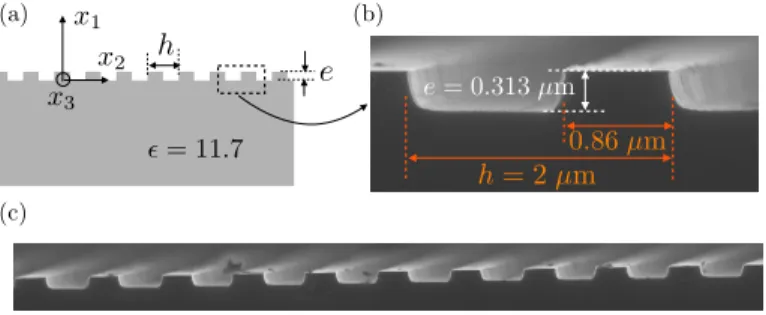
h = 2 µm e = 0.313 µm 0.86 µm (a)
e
= 11.7h
(b) (c) x2 x1 x3Fig. 1.(a) Periodic rough interface between air and a dielectric, (b) SEM view of the realized sample with Silicium, (c) shows a lager view of the interface.
roughnesses, boundary layer effects are of the order(kh), with k the wavenumber while the propagation effects are of the order(ke).
Subwavelength structurations, as roughnesses, satisfy kh⌧1; next, for deep roughnesses ke=O(1) kh, thus the boundary layer effects are negligible compared to the propagation effects; however, when(ke)decreases, they may become of the same order and eventually dominant. A discussion on the validity of the homogenization in the bulk (layer model) compared to the homogenization of the interface (interface model) can be found in [10,11] in the case of arrays made of a perfect conductor.
The interface model is presented in Section2. For transverse magnetic polarization of light in two dimensions, we derive the effective jump conditions across an equivalent interface of thickness e, Eqs. (22) which involve two parameters(B,C)characteristic of the roughnesses (it is worth noting that the interior of the interface is not questioned). The reflection coefficient for an incident plane wave at oblique incidence is deduced, Eq. (26). For comparison, we give the reflection coefficient in a layer model, (31), similar to that given by the anisotropic Bruggeman model. In Section4, the validity of the models is inspected by comparison with direct numerical calculations based on modal method [12] and with experimental measurements. The results show that the interface model is able to accurately describe the scattering properties of small roughnesses when their actual geometry is considered in the model. In comparison layer models overestimate the effect of the roughnesses, leading to a larger shift in the Brewster phenomenom. The discrepancy between layer and interface models is discussed in Section5in the light of calculations performed for varying roughness thicknesses.
2. HOMOGENIZATION OF PERIODIC SLIGHTLY ROUGH SURFACE
We consider a periodic rough interface x1= f(x2)invariant along x3separating the air from a dielectric region with relative permittivity
#r. We shall see that within the framework of homogenization theory, the periodic roughnesses of thickness e and spacing h can be
replaced by an equivalent interface of same thickness across which effective jump conditions apply. We start with the wave equation written for the magnetic field H(x)(x= (x1, x2)) being polarized along e3, which reads as
div 1
#(x)rH(x) +k
2H(x) =0, (1)
where #(x)is the relative permittivity which depends on space; we denote #(x) =# =#rin the dielectric and #(x) =#+ =1 in the air,
and k= p#0µ0wis the wavenumber in the air. To Eq. (1), we have to associate boundary conditions. The boundary conditions at
the air/dielectric interface are the continuities of H and of 1/#rH·n. Finally, once the incident wave has been defined, radiation
conditions apply for the scattered field; for the time being, we do not need to specify them. For simplicity, we shall work with the field C such that (1) is written
divC(x) +k2H(x) =0, C(x)⌘ 1
#(x)rH(x), (2)
with boundary conditions being now the continuities of H and of C.n at the air/dielectric interface. It is easy to see that the electric field E= (E1, E2, 0)can be deduced from C, with
C1= iw E2, C2=iw E1, (3)
(the continuity of the normal component of C corresponds to the continuity of the tangential component of E).
As in the classical homogenization, we shall work using two systems of coordinates. Without loss of generality, we consider k=O(1), h=h⌧1, (4)
and we have e=O(h). Thus x= (x1, x2)is the coordinate at the macroscale 1/k, and we define the coordinate
y=x/h, (5)
the coordinate at the microscale h. Fig. 2shows the resulting rescaling in y coordinates of the elementary cell Y = ( ym 1, ym1)⇥
( 1/2, 1/2); the value of ym
1 >e/(2h)is incidental, since we shall consider the limit ym1 !• in practice. We define also Y+and Y
1
e/2h e/2h 0 ym 1 ym 1y
1y
2S
Y
Fig. 2.Elementary cell in(y1, y2)coordinates. Y= ( y1m, ym1)⇥ ( 1/2, 1/2)(and the limit ym1 !• will be considered in practice);
Y+and Y are the subregions of Y occupied by the air (#+ =1) and by the dielectric (# =#
r) respectively.
A. Expansions of the solution in the near and far fields and matching conditions
A.1. Near and far field expansions
The idea is to define two different expansions of(H, C)in the far field and in the near field of the roughnesses. In the far field, we use H=H0(x) +hH1(x) +· · ·, C=C0(x) +hC1(x) +· · ·, (6)
with the terms in the expansions depending on x only which is adapted to describe the variations of the propagating waves (they vary on the wavelength scale 1/k). In the near field, we use
H=h0(y,x2) +hh1(y,x2) +· · ·, C=c0(y,x2) +hc1(y,x2)· · ·. (7)
with a dependence on y adapted to describe the variations of the non propagating waves (or evanescent waves) at the scale h and a dependence on x2adapted to describe the variations of the propagating waves along the roughnesses. The terms hnand cn, n=0,· · ·,
are assumed to be periodic with respect y2. This tells us that the field at the microscale is repeated from one cell to the other while long
scale variations, at the scale of the wavelength, are handled by x2. Eventually, the Eqs. (2) will be written at the orders h 1and h0in
the near field, and at the orders h0and h1in the far field, using the differential operators which take the forms
8 > < > :
r ! rx, in the far field,
r ! 1
hry+
∂
∂x2 e2, in the near field.
(8)
A.2. Matching conditions
From a unique problem, we have build two applying in two different regions. Thus, we have to associate to each problem boundary conditions in order that they are well-posed. The boundary conditions on the roughnesses apply in the near field only (at each order in h) while the radiation conditions apply in the far field only. Thus, there are missing boundary conditions in the near field when y1 ! ±• which are the equivalent of the radiation conditions; reversely there are missing conditions in the far field when
x1 ! 0±, which correspond to the equivalent conditions that we are looking for (these conditions encapsulate the effect of the
roughnesses). These missing boundary conditions are provided simultaneously by the so-called matching conditions which ensure the continuity of H and C in an intermediate region where the evanescent field can be considered as negligible, typically when
|x1| ⇠O(ph)!0 and thus|y1| ⇠O(1/ph)! +•. We thus write that H0(x) +hH1(x)⇠h0(y,x2) +hh1(y,x2)in this intermediate
region, and identify the limits at each order in h. Owing to the Taylor expansions H0(x1, x2) =H0(0+, x
2) +x1∂x1H0(0+, x2) +· · · =
H0(0+, x2) +hy
1∂x1H0(0+, x2) +· · · (same for C0), we get at the order 0
H0(0±, x2) = lim ym 1!+• h0(±y1m, y2, x2), C0(0±, x2) =ymlim 1!+• c0(±y1m, y2, x2), (9)
and at the order 1,
8 > > > < > > > : H1(0±, x2) = lim ym 1!+• h1(±ym1, y2, , x2)⌥ym1 ∂H 0 ∂x1(0 ±, x2) , C1(0±, x2) =ymlim 1!+• c1(±ym 1, y2, , x2)⌥ym1 ∂C 0 ∂x1(0 ±, x2) . (10)
Finally, something has to be said on the variations of #. In the far field regions x1<0 and x1>0, #=# and #=#+are constant
since the far fields do not contain the roughness region. The variations of # concern the near field only, and being periodic, we simply have #(y)with no long scale variation of # with x2and with
lim
ym 1!+•
#(±ym
B. The leading and first order solutions and the associated jump conditions
B.1. The solution at the order 0
In the near field, (2) givesryh0=0 at leading order, in h 1. It follows that h0does not depend on y and, from the first matching
condition in (9), we deduce that
h0(x2) =H0(0±, x2). (12)
From (2), we also have divyc0=0. Integrating this equation over Y and owing to the continuities c0·n at the air/dielectric interface
and to the periodicity of c0w.r.t y
2, we getRdy2c01(ym1, y2, x2) =Rdy2c01( ym1, y2, x2). Then, it is sufficient to take the limit ym1 ! +•
in the second matching condition of (9) to get
C10(0+, x
2) =C10(0 , x2). (13)
At the dominant order, the roughnesses are not visible: the rough interface is equivalent to a flat interface between the air and the dielectric, with the continuities of H0and of C0
1, which correspond to the usual continuities of the magnetic field and of the tangential
component of the electric field from (3). To capture the effect of the roughnesses, we need to go to the next order.
B.2. Elementary problems
Before going to the next order, elementary problems have to be defined, which will make the effective interface parameters to appear. To that aim, we focus on the problem satisfied by h1, which, from (2), reads as
8 > > < > > : divyc0=0, with c0= 1 #(y) ryh1+∂H 0 ∂x2(0, x2)e2 , lim y1!±•ryh 1=#±C0 1(0, x2)e1, (14)
with boundary conditions being the continuities of h1and of c0.n at each air/dielectric interface. To get (14), we have used C =
1/#rxH written at the order h0for the near field solution, and h0(x2) =H0(0, x2)from (12). We also used the matching conditions
c0(±•, y2, x2) =C0
1(0, x2)e1+1/#±∂x2H0(0, x2)e2in (14) to get the limits ofryh1. The problem (14) is linear w.r.t ∂x2H0(0, x2)and
C0
1(0, x2), thus we can write
h1(y,x2) =C01(0, x2)h( 1 )(y) +∂H 0
∂x2 (0, x2)h
( 2 )(y) +ˆh(x
2), (15)
and h1is solution of the problem (i) for any incident wave (thus any values of ∂x2H0(0, x2)and C01(0, x2)) if h( 1 )satisfies
div 1 #(y)rh ( 1 ) =0, lim y1!±•rh ( 1 )= #±e1, (16) with h( 1 )being a y
2-periodic and continuous and with 1/#(y)rh( 1 ).n being continuous at the air/dielectric interface, and (ii) if h( 2 )
satisfies div 1 #(y)r(h ( 2 )+y 2) =0, ylim 1!±•rh ( 2 )=0, (17) with h( 2 )being a y
2-periodic and continuous and with 1/#(y)r(h( 2 )+y2).n being continuous at the air/dielectric interface. The
so-built elementary solutions(h( 1 ), h( 2 ))are defined up to a constant and can be written
h( 1 )(y) = 8 < : # y1+B +hev(1)(y), #+y1+B++hev(1)(y), y1<0, y1>0. and h( 2 )(y) =h(2) ev(y), (18) where h(1)
ev and hev(2))are evanescent fields vanishing at y1! ±•. Indeed, for symmetric shapes of roughnesses, h( 2 )is an odd function
of y2, while h( 1 )is even, thus this latter has possibly two different constants at y1 ! ±•. The evanescent fields, as the constant
B+ B , depend on the shape of the roughnesses and on #
rand the problems have to be solved numerically; we shall see in the
following section that these elementary solutions make the interface parameters to appear.
B.3. Solution at order 1
The limits H1(0±, x2)directly follows from the first matching condition in (10), using (15) along with (18). Specifically, using that
∂x1H0(0±, x2) =#±C10(0, x2), we easily obtain that
8 < : H1(0+, x2) =B+C0 1(0, x2) +ˆh(x2), H1(0 , x 2) =B C01(0, x2) +ˆh(x2). (19)
Now, we need to determine the jump in C1
1. To do so, we start by integrating over Y the first equation of Eqs. (2) written at order 0 in h,
that is Z Ydy " divyc1+ ∂c 0 2 ∂x2+H 0(0, x 2) # =0. (20)
We haveRYdivyc1=c11(ym1) c11( y1m)using the continuity of c1.n and the periodicity of c1. Next, with c02=1/#⇥∂y2h1+∂x2H0(0, x2)
⇤ from (14), and using (15), it is straightforward to obtain that
C11(0+, x 2) C11(0 , x2) = eh(1 f)✓ 1#+ 1 # ◆ + Z Y dy #(y) ∂h( 2 ) ∂y2 (y) ∂2H0 ∂x2 2 (0, x2), (21)
with f the filling fraction of the roughnesses, thus the surface of the roughness equal toS =eh f . In the matching conditions (10), we used that(1/#±)∂2
x2 2H
0+k2H0= ∂x
1C01at x1=0±respectively. Eventually, we also used that h( 1 )is even, from which the integral of
∂y2h( 1 )over Y vanishes.
B.4. Final jump conditions and interface parameters
To get the final form of the jump conditions, we need two additional steps. First, the conditions (12)-(13) at the order 0 and the conditions (19)-(21) at the order 1 are used to write the jump conditions on(H0+hH1)and on(C10+hC11)which admit the same expansions as
H and C up to O(h2), and at this stage, the jumps have been expressed across a zero thickness interface, namely between x1=0 and
x1=0+. It has been previously discussed that restoring the thickness of the actual interface improves the accuracy of the model, see e.g.
[13,14]. This is done by "enlarging" the equivalent interface; to do that, we define H±=H(±e/2, x2), and H=1/2(H++H ) +O(e)
with e=O(h)(the same for C±). Next, the jump JHK⌘H+ H =H(0+, x2) H(0 , x2) +e∂x
1H+O(e2), where we have used
Taylor expansions of H(±e/2, x2). The jump conditions at the new equivalent interface of thickness e finally read as
8 > > > > < > > > > : H+ H = hB 2 1 # ∂H ∂x1 + 1 #+ ∂H+ ∂x1 , 1 #+ ∂H+ ∂x1 1 # ∂H ∂x1 = hC 2 " ∂2H ∂x22 + ∂2H+ ∂x22 # ek2 2 ⇥ H +H+⇤, (22)
with(B,C)the interface parameters defined by 8 > > > < > > > : B = B+ B +2he #+#+ , C = Z Y dy #(y) ∂h( 2 ) ∂y2 + e h ✓ f #+ + 1 f # ◆ . (23)
3. REFLECTION BY A PERIODIC ROUGH INTERFACE
In this section, we give the reflection coefficient of an incident plane wave predicted by our interface model. For comparison, we also give the reflection coefficient predicted by a classical layer model, corresponding to the two-scale homogenization in the bulk of the roughnesses.
A. The interface model for roughnesses
Using the Fresnel notations, and with a time dependence eiwt, the solution in the homogenized problem reads as
H(x1, x2) =
8 < :
h
eia(x1+e/2) r e ia(x1+e/2)ie ibx2, x
1>e/2,
t eig(x1 e/2)e ibx2, x
1< e/2,
(24)
with
a=k cos q, b=k sin q, and g=kp# sin2q. (25)
It is worth noting that the region e/2<x1<e/2 is not considered since the jump conditions (22) do not question this region and
allows to determine the scattering coefficients(rTM, tTM)unambiguously (the homogenized problem is simply one dimensional along
x1). The reflection coefficient reads as
rTM= z1 z2 z1+z2, with 8 > > > < > > > : z1= g# (hCb2 ek2) ✓ i hB 4 g # ◆ , z2=a 1+ihBg # + (hCb 2 ek2)hB 4 . (26)
At the dominant order, we recover the reflection coefficient of a flat interface r0= (g# a)/(g#+a)vanishing at the Brewster angle
qB=atan p# . (27)
Then, it is easy to see that the reflected field does not vanish near the Brewster angle but presents a minimum rminat q=qB+O(h2),
with rmin=i2pkh #+1 h (1+#)e h B #C i . (28)
B. The classical layer model
When the classical homogenization is sought, the case of layered media yields a simple solution in the form of an equivalent homogeneous and anisotropic medium [15] and e.g. [16,17] for practical applications. The anisotropic medium is characterized by
(#k, #?)given by #k= f #++ (1 f) # , #? =f # ++ (1 f)# . (29)
When considering the problem of the scattering of an incident plane wave for a layer of thickness e made of such effective medium and sandwiched between the substrate and the air, the component of the wavenumber along x2in the layer is
d=q#k(k2 b2/#
?), (30)
being the equivalent of the component g in the substrate, (25), and the reflection coefficient ˜r reads as 8 > > < > > : ˜r= i tan(de)(1 x1x2) + (x1 x2)) i tan(de)(1+x1x2) (x1+x2), with x1=#kad, x2= #k # g d. (31)
While this classical homogenization leads to accurate results when e is large, which means of the order of magnitude or larger than the wavelength, it is not efficient to predict the scattering properties of a layer with ke⌧1. We shall illustrate this failure in the following section.
4. NUMERICAL AND EXPERIMENTAL VALIDATION
A. Realization and characterization of the sample and ellipsometric measurements
A grating was realized on a Si substrate using optical lithography. The pattern was obtained using Direct Writing Lithography with a focused laser beam at 405 nm defining the lines in a positive resist. This process allowed achieving a linewidth resolution of approximately 1 µm over an area of 1⇥2 cm2. After development, the Si was etched using Reactive Ion Etching (RIE), with a limited process time so that vertical walls were obtained.
The measurements of the scattering properties were performed on a Woollam WVASE ellipsometer. Ellipsometry measures the ratio of the reflexion coefficients rTMin TM polarization and rTEin TE polarization, specifically
r= rTM
rTE
=tan y eij, (32)
with j=jTM jTEthe phase shifts after reflexion in TM and TE polarizations, and Y=atan(|rTM/rTE|)the so-called ellipsometric
angle. The ellipsometer was equipped with a Fourier Transform InfraRed spectrometer as a source. The measurements were performed in the 2-20 µm range with a resolution of 32 cm 1and at different angles selected as to follow the ellipsometric angles evolution
across the Brewster’s angle. In the following, we shall analyze the results for l>5 µm, below which higher interference orders appear, leading to Rayleigh Wood anomalies. In fact, the interference order -1 appears in the substrate at l=9 µm, but we checked numerically that this does not affect significantly the 0 order.
Eventually, after the measurement were done, the sample was cleaved to allow for accurate measurements of the grating profile in Scanning Electron Microscopy (SEM), see Fig.1. From the different realized SEM profiles, the shape of the periodic roughnesses appears to be almost rectangular, of width 0.86 µm for a grating periodicity h=2.0 µm, whence f =0.43, and of depth 0.313 µm. For this geometry, and with #r=11.7, we computed(B,C)defined by (23) and entering in the jump conditions (22) by solving the
elementary problems (16) and (17), and found
B =0.519, C =0.061, (33)
which provide the reflection coefficient in (26) without any ajustable parameter. For the layer model, we have from (29) that #k=0.607 and #?=0.178, from which the reflection coefficient in (31) is known (also without any ajustable parameter).
B. Typical measurements of the reflection, the pseudo Brewster angle
From now on, we shall use the angles(y, j)to characterize the modulus and the phase of the reflection coefficient. For reference calculations, we use direct numerics in TM and TE polarizations using a modal method similar to the RCWA [12]. Finally, to avoid additional discussion of the models, we use(r, ˜r)in Eqs. (26) and (31) from the models in TM polarization, and the reflection coefficient
given by the modal calculation in TE polarization.
We start by reporting in Fig.3typical variations of y and j as a function of q (for l=5, 10, 15 and 20 µm). The experimental measurements (open circles) are compared to the modal calculations (dashed lines) and to (i) the interface model (26) (plain lines) and (ii) the layer model (31) (dotted lines). As expected, the agreement between the modal calculations and the experiments is excellent. Next, the accuracy of the interface model is very good without any ajustable parameter, and expectedly it is better and better for larger and larger wavelengths. Note that this is a good news since our frequency range did not fulfilled a priori the low frequency regime corresponding to h=kh⌧1: indeed, with h=2 µm, wavelengths l=5, 10, 15, 20 µm correspond to h=2.5, 1.3, 0.8, 0.6, which
reveals an unexpected robustness of the interface model. In comparison, the layer model, without adjustable parameter, predicts significantly larger shifts of the Brewster effect than the measured ones. This overestimate of the effect of the roughnesses is confirmed using classical retrieval procedures based on EMA models (Effective Medium Approximation) of the Bruggeman type. In this case, the set of measured reflection coefficients is used in an inverse problem to retrieve(e, f). Assuming in the EMA an equivalent isotropic layer filled with small spheres, the retrieved thickness is e=0.256 µm, and assuming an equivalent anisotropic layer filled with stems, the retrieved thickness is e=0.239 µm, thus about 20% smaller than the actual thickness (for both EMA, the filling fraction is correctly found, with f '0.44). 0 60 120 180 0 15 30 45 = 5 µm = 10 µm = 15 µm = 20 µm 50 0 80 ( ) ( ) ( ) 50 0 80 ( ) 50 0 80 ( ) 50 0 80 ( )
Fig. 3.Variation of y and j as a function of the incidence q for l =5, 10, 15 and 20 µm. Experimental measurements (blue open symbols), direct modal calculation (red dotted lines), interface model (26) (black plain lines) and classical layer model (31) (green dotted lines). For the interface and layer models, we used the actual dimensions of the sample e=0.313 µm, h=2 µm and f =0.43 (without ajustable parameters).
C. Characterization of the shift in the Brewster effect
From the profiles of(y, j), it is possible to quantify the shift in the Brewster effect. We report in Fig.4the minimum in the reflection modulus as a function of l (to find such minimum from the experimental profiles in Figs.3, we used a spline interpolation of the data). Again, the modal calculations and the experimental results are in good agreement. The prediction from our interface model for l>5
µm is rather good when compared to both the numerics and the experiments, and as previously said, it is more accurate for larger
wavelength; specifically, the discrepancy with the experimental results ranges between 0.3 and 1.4 , corresponding to relative errors of 5 to 20%. Finally, the minimum of reflection follows reasonably a power law in 1/l according to our estimate of rmin, (28) (this latter is
reported in dashed-dotted line, and the relative better agreement with the experiments is casual). In comparison, the layer model predicts a much higher reflection, with y being about twice the actual one (and with a discrepancy ranging from 5 to 10 , the relative error is always larger than 100%).
We now move on a more subtil effect, which is the deviation in the Brewster angle qBto the pseudo Brewster angle qPB. In Figs.5,
we considered two different estimations of qPB, namely (i) the angle at the minimum of the reflection modulus min(y)and (ii) the angle
realizing j=90 (and to avoid multiple notations, we term both qPB). Obviously, the first criterion is intuitively the more adapted to
measure the shift with respect to a vanishing reflection. On the other hand, the second criterion is often used to characterize a sudden change in the scattering response, as resonance phenomena, and it has the advantage to be very precise since the large variation in the reflection phase occurs in a very short angle range (this is visible in Figs.3). This is indeed what we observe, with a dispersion in the results coming from the experimental data much more important in Fig.5(a) than in Fig.5(b). Although the interface model captures the variations in qB qPBmore accurately than the layer model, this agreement remains qualitative. Indeed, the deviation in
10 20 10 (µm) 5 15 20 0 mi n( ), ( )
Fig. 4.Minimum of the reflection modulus y as a function of l. From the experimental measurements (open symbols), the modal calculations (red dotted lines), the interface model (26) (black plain lines, the black dashed-dotted shows the approximated result, (28)) and the classical layer model (31) (green dotted lines).
B PB ( ) 0 10 (µm) 5 15 20 4 8 12 PBfor min( ) B PB ( ) 0 10 (µm) 5 15 20 4 8 12 PBfor = 90 (a) (b)
Fig. 5.Deviation qB qPBof the Brewster angle as a function of the wavelength, (a) at the minimum in y and (b) at j=90 . Same
representation as in Fig.4.
predict a shift at the order O(h) =O(1/l), but we reach the limit of validity of the model derived up to O(h2)(to get quantitative predictions, one should derive the model up to O(h3)). Incidentally, although the two deviations look similar, they differ in O(1/l2)
law, which means that the angles realizing the minimum of reflection and realizing the 90 - reflection phase differ at the dominant order.
5. NUMERICAL STUDY OF THE INFLUENCE OF THE ROUGHNESS THICKNESS
We have stated and illustrated that the interface model is adapted to small roughness thicknesses (ke⌧1) while the layer models, as the Maxwell-Garnett model, the EMA or the model of layered medium presented in the Section3.Bare adapted in the opposite limits (ke 1). In this section, we show in more details what is happening when increasing the roughness thickness. To do so, we use comparison of the models with direct numerics; for simplicity, we consider rTMwhich is available from the direct numerics, and which
is the prediction given in the models, Eqs. (26) and (31).
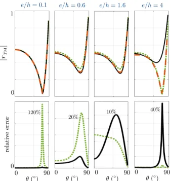
We computed the variations of rTMas a function of the incidence q for a fixed frequency corresponding to kh=0.5 and increasing
the value of e/h. Results are reported in the top panels of Figs.6. We observe 3 behaviors: for small thicknesses e/h, the interface model is the most accurate (e/h=0.1) and we shall be more explicit since at this stage, this is not obvious by simple inspection of the plot. For intermediate e/h values, both models experience a transition : the layer model becomes more and more accurate while the interface model becomes less and less accurate (e/h=0.6 and 1.6). Eventually, for large e/h values, the layer model becomes clearly the most accurate (e/h=4).
From the top panels of the Figs.6, the layer model appears reasonably predictable for all e/h values if we are interested in the overall behavior of the reflection over the range(0, 90 ). The reason is simple: because the effect of the roughnesses vanishes for vanishing e/h, the reflection for small e/h is merely the same as for a flat interface, and this is obtained in both models. But if we are precisely interested in the small variations with respect to the flat case, we want to be predictable when they are the most significant,
e/h = 0.1 e/h = 0.6 e/h = 1.6 e/h = 4 0 0 ( ) 0 90 120% 20% 10% 40% re lat iv e er ror 1 |rTM | ( ) 0 90 ( ) 0 90 ( ) 0 90
Fig. 6.Comparison of the layer and interface models for increasing e/h values. The top panels report the variations of y as a func-tion of q (open symbols: direct numerics, plain lines: interface model, dashed lines: layer model. The bottom panels reports the relative errors in y in the two models.
that is near the Brewster angle. The bottom panels in Fig.6show the relative errors, which allows to specify the accuracy of the models. For e/h=0.1, the layer model appears to be unable to describe quantitatively the small shift in rTMnear the Brewster angle,
reaching an error larger than 100%; outside this region, the error does not exceed 2% but this small discrepancy is precisely of the same order of magnitude than the small shift with respect to the flat case. To the contrary, the interface model keeps a very small error over the whole range (0,90 ), with a maximum of 1.5% at the Brewster angle, otherwise less than 0.1%. Next increasing e/h produces an increasing effect of the propagation effect against the boundary layer effect, and the error in the layer model becomes more and more accurate while the interface model becomes less and less accurate.
6. CONCLUSION
In this work, we have proposed and validated an interface model able to describe accurately the scattering of light by periodically roughnesses with small thickness. The typical range of validity of the model is kh<1 and e/h<1, although we observed that the model remains surprisingly predictive up to the first Rayleigh-Wood anomaly (in the experiments at l=5 µm). In comparison,
classical layer models which consist in replacing the roughnesses by a layer filled with an effective medium are not predictive at all when the direct problem is sought.
Of course, retrieval methods can be used in which an effective thickness and an effective filling fraction are used as free parameters. However, the use of such methods is questionable if the retrieved parameters are far from the actual ones and we have seen that the retrieved thickness was significantly underestimated in our experiments (about 20%). This is why we think that the use of such layer models is unadapted. Indeed, once a retrieved thickness has been obtained for a given sample, it is not obvious that doubling the sample thickness leads to doubling the effective thickness, and if it is not the case, the retrieval method becomes simply ad hoc since it does not allow to anticipate other sample responses. More generally, tempting a model in a retrieval procedure without having validated the model in the direct problem is hazardous; it may lead to multiple local minima in the space of the retrieved parameters which simply reflect the inadequation between the real system and the model that we impose to it.
ACKNOWLEDGMENTS
The authors thanks Kim Pham for fruitful discussions. A.M. and J.-J.M. acknowledge the financial support of the french Mission Interdisciplainare du Centre National de la Recherche Scientifique (MI/CNRS) under grant INFYNITI/PomS.
REFERENCES
1. M. Saillard and D. Maystre, “Scattering from metallic and dielectric rough surfaces,” JOSA A 7, 982–990 (1990).
2. M. Saillard, “A characterization tool for dielectric random rough surfaces: Brewster’s phenomenon,” Waves in random media 2, 67–79 (1992). 3. J.-J. Greffet, “Theoretical model of the shift of the brewster angle on a rough surface,” Optics letters 17, 238–240 (1992).
4. C. Baylard, A. A. Maradudin, and J.-J. Greffet, “Coherent reflection factor of a random rough surface: applications,” JOSA A 10, 2637–2647 (1993). 5. A. Maradudin, R. Luna, and E. Méndez, “The brewster effect for a one-dimensional random surface,” Waves in Random Media 3, 51–60 (1993).
6. T. M. Elfouhaily and C.-A. Guérin, “A critical survey of approximate scattering wave theories from random rough surfaces,” Waves in Random Media 14, R1–R40 (2004).
7. J. Nevard and J. B. Keller, “Homogenization of rough boundaries and interfaces,” SIAM Journal on Applied Mathematics 57, 1660–1686 (1997). 8. G. Kristensson, “Homogenization of corrugated interfaces in electromagnetics,” Progress in electromagnetics research 55, 1–31 (2005). 9. A. H. Sihvola, Electromagnetic mixing formulas and applications, 47 (Iet, 1999).
10. J.-J. Marigo and A. Maurel, “Second order homogenization of subwavelength stratified media including finite size effect,” SIAM Journal on Applied Mathematics 77, 721–743 (2017).
11. J.-J. Marigo and A. Maurel, “An interface model for homogenization of acoustic metafilms,” Chap. 7, World Scientific Publishing, Edts. R. Craster and S. Guenneau (2017).
12. A. Maurel, J.-F. Mercier, and S. Félix, “Wave propagation through penetrable scatterers in a waveguide and through a penetrable grating,” The Journal of the Acoustical Society of America 135, 165–174 (2014).
13. A. Maurel, J.-J. Marigo, and A. Ourir, “Homogenization of ultrathin metallo-dielectric structures leading to transmission conditions at an equivalent interface,” The Journal of the Optical Society of America B 33, 947–956 (2016).
14. J.-J. Marigo, A. Maurel, K. Pham, and A. Sbitti, “Effective dynamic properties of a row of elastic inclusions: the case of shear waves,” Journal of elasticity (2017).
15. A. Bensoussan, J.-L. Lions, and G. Papanicolaou, Asymptotic analysis for periodic structures, vol. 5 (North-Holland Publishing Company Amsterdam, 1978).
16. A. Maurel, S. Félix, and J.-F. Mercier, “Enhanced transmission through gratings: Structural and geometrical effects,” Physical Review B 88, 115416 (2013). 17. A. Akarid, A. Ourir, A. Maurel, S. Félix, and J.-F. Mercier, “Extraordinary transmission through subwavelength dielectric gratings in the microwave range,”