www.clim-past.net/12/1765/2016/ doi:10.5194/cp-12-1765-2016
© Author(s) 2016. CC Attribution 3.0 License.
Testing the impact of stratigraphic uncertainty on spectral
analyses of sedimentary series
Mathieu Martinez1, Sergey Kotov1, David De Vleeschouwer1, Damien Pas2, and Heiko Pälike1
1MARUM, Centrum for Marine Environmental Sciences, Leobenerstr., Universität Bremen, 28359 Bremen, Germany 2Pétrologie sédimentaire, B20, Géologie, Université de Liège, Sart Tilman, 4000 Liège, Belgium
Correspondence to:Mathieu Martinez ([email protected])
Received: 17 December 2015 – Published in Clim. Past Discuss.: 29 January 2016 Revised: 22 July 2016 – Accepted: 18 August 2016 – Published: 2 September 2016
Abstract.Spectral analysis is a key tool for identifying peri-odic patterns in sedimentary sequences, including astronom-ically related orbital signals. While most spectral analysis methods require equally spaced samples, this condition is rarely achieved either in the field or when sampling sediment core. Here, we propose a method to assess the impact of the uncertainty or error made in the measurement of the sample stratigraphic position on the resulting power spectra. We ap-ply a Monte Carlo procedure to randomise the sample steps of depth series using a gamma distribution. Such a distribu-tion preserves the stratigraphic order of samples and allows controlling the average and the variance of the distribution of sample distances after randomisation. We apply the Monte Carlo procedure on two geological datasets and find that gamma distribution of sample distances completely smooths the spectrum at high frequencies and decreases the power and significance levels of the spectral peaks in an important pro-portion of the spectrum. At 5 % of stratigraphic uncertainty, a small portion of the spectrum is completely smoothed. Tak-ing at least three samples per thinnest cycle of interest should allow this cycle to be still observed in the spectrum, while taking at least four samples per thinnest cycle of interest should allow its significance levels to be preserved in the spectrum. At 10 and 15 % uncertainty, these thresholds in-crease, and taking at least four samples per thinnest cycle of interest should allow the targeted cycles to be still observed in the spectrum. In addition, taking at least 10 samples per thinnest cycle of interest should allow their significance lev-els to be preserved. For robust applications of the power spec-trum in further studies, we suggest providing a strong control of the measurement of the sample position. A density of 10 samples per putative precession cycle is a safe sampling
den-sity for preserving spectral power and significance level in the Milankovitch band. For lower sampling density, the use of gamma-law simulations should help in assessing the im-pact of stratigraphic uncertainty in the power spectrum in the Milankovitch band. Gamma-law simulations can also model the distortions of the Milankovitch record in sedimentary se-ries due to variations in the sedimentation rate.
1 Introduction
Spectral analysis methods have become a key tool for iden-tifying Milankovitch cycles in sedimentary series and are a crucial tool in the construction of robust astronomical timescales (Hinnov, 2013). The climatic or environmental proxy series that form the subject of spectral analyses are generally the result of measurements on rock samples col-lected from a sedimentary sequence, consisting of cores or outcrops. Most of spectral analysis methods (Fourier Trans-forms and derivatives, such as the multi-taper method) re-quire equally spaced depth or time series, which implies that samples need to be taken at a constant sample step (Fig. 1a). Unfortunately, this is rarely achieved, especially for sedimen-tary sequences sampled in outcrops (e.g. Fig. 1b–c and e). Often, an uncertainty of ∼ 5–15 % is observed in the thick-ness or distance measurements, even when using a Jacob’s staff (Weedon and Jenkyns, 1999). In core sediments, uncer-tainties in the sample position are also observed when per-forming physical sampling at very high resolution or because of core expansion phenomena (Hagelberg et al., 1995) or im-perfect coring (Ruddiman et al., 1987).
Although uncertainties exist regarding the actual posi-tion of samples, few case studies document their effect on
Ideal sampling
pattern Real samplingpattern
0.1 0.15 0.2 0.25 0.3 0 20 40 60 80 250 Sample distance (m) Real distribution of sample distance
in the La Charce series
Distribution
(a) (b)
Constant
sample distance Sample distance not constant
Lithology Sample location (c) (e) 0 100 200 300 400 500 600 Distribution 0.1 0.15 0.2 0.25 0.3 Sample distance (m) (d) Ideal distribution of sample distance
(sample distance = 0.20 m) Level (m) 10 20 30 40 50 60 70 80 90 100 110 GRS (ppm eU) 5 6 7 8 9 10 11 12 13 14
Sample distance fixed at 0.20 m Sample position from Martinez et al. (2013)
Figure 1.Illustration of the problem. (a) Theoretical sedimentary log with position of samples in an ideal case in which the samples are
strictly equally distant. (b) Theoretical sedimentary log with position of samples in a common sampling pattern where all samples are not strictly equally distant. Here the error in the sample position is exaggerated for the purpose of the example. (c) The gamma-ray series from La Charce shown as if all samples were strictly equidistant (black curve) and as they are positioned in Martinez et al. (2013) (red curve). (d) Distribution of sample distances in the case of ideal sampling of the La Charce series (all sample distances are fixed at 0.20 m). (e) Distribution of sample distances in the case of the La Charce series as published in Martinez et al. (2013).
the identification of periodic patterns. Moore and Thomson (1991) recognised that perturbations of the regular sampling scheme (i.e. jittered sampling) impact the power spectrum by reducing spectral power in the high frequencies. Huybers and Wunsch (2004) and Martinez and Dera (2015) address an analogous problem by assessing the effect of sampling un-certainty on the age model of a calibrated time series that is plotted against numerical age. However, none of these studies explicitly addresses the impact of errors in the measurement of the sample position on uncertainties in the power spec-trum amplitudes. In this study, we address this problem by quantifying the impact of such errors on the frequency and power distribution. Therefore, we provide a new procedure that is based on a Monte Carlo approach for randomising the distance between two successive samples in a sedimentary series. The resulting simulated series are subsequently used to assess the impact of the sample-position error on spectral analyses. We first apply the procedure to a theoretical exam-ple and then to two previously published geological datasets, one sampled as regularly as possible and another sampled irregularly.
2 The error model
In this paper, the term “stratigraphic uncertainty” refers to the uncertainty of the sample positions. Testing the impact of the stratigraphic uncertainty on the spectral analyses re-quires a randomisation procedure that reflects typical errors made during measurements of the stratigraphic position of samples. Figure 1c to e illustrate the consequences of the stratigraphic uncertainties on a geological series (here the La Charce series; see Sect. 3.1). Figure 1c compares the real sampling made on this series (in red) to an ideal sampling in which samples are taken at a strictly even sample distance (in black). Errors in the sample positions distort the sedi-mentary series: some intervals are compressed while some others are increased. Ideally, all sample distances should be strictly the same, so that the distribution of sample distances should be concentrated on only one value (Fig. 1d). In real-ity, as uncertainties exist regarding the sample positions, the sample distances show a distribution over a certain range of values, which depends on the accuracy with which the dis-tance measurements have been taken (Fig. 1e). In the case of the La Charce series, the standard deviation of the sample distances is assessed at 12.5 % of the average sample dis-tance (the method to estimate this standard deviation is pro-vided in Sect. 4). If the error in the distance measurement was systematic, one should expect the same level of error in
the total length of the series. However, in total, the differ-ence in the length of the series between the ideal case (all sample distances strictly the same) and the real case is only 1.4 % of the total length of the series (Fig. 1c). Each sample distance is measured independently of the other sample dis-tances, so that each measurement can overestimate or under-estimate the real distance between two successive samples. The errors thus compensate for each other, implying that the process at the origin of the error measurements is not system-atic but random.
Three conditions must be respected to design the error model: (i) the stratigraphic order of samples is hard-set and must not be changed by the randomisation process (e.g. Fig. 1c); (ii) the average and standard deviation of sample steps must be maintained during the randomisation process; (iii) the error model must be random. These conditions can be achieved if the error model randomises the sample distances rather than the sample positions. In that case, the probability density function should have a positive and continuous dis-tribution (i.e. values obtained after randomisation are contin-uous and positive). In addition, the average sample step and the standard deviation of the distance between two succes-sive samples are known and should be parameterised.
The gamma distribution fulfils all these conditions. The gamma distribution is continuous and has a positive support. Parameters k and 2 respectively define the shape of the dis-tribution and its range of values. The mean (E) of the density of probability is defined as (Burgin, 1975)
E = k · 2 (1)
and its variance (σ2) as
σ2=k · 22=E · 2. (2)
Both the mean (E) and the variance (σ2) are known, as they correspond to the mean and variance of the sample steps, and they can be quantified in the field (see Sect. 4 for a discussion on the variance of sample steps). Therefore, k and 2 can be parameterised using the following relations:
2 = σ
2
E, (3)
k =E
2. (4)
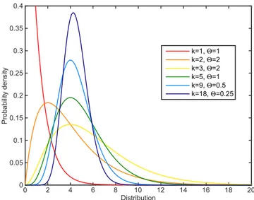
Various gamma probability density functions are shown in Fig. 2. A high variance-to-mean ratio corresponds to a high 2-parameter value compared to the k parameter. The result-ing density probability function corresponds to an exponen-tial probability function in the most severe and spectrum-destructive case. This distribution corresponds to sampling conditions during which no control was exerted on the strati-graphic position of samples, so that the uncertainty in the sample position is at a maximum. Obviously, this situation is not a realistic case to reflect geological practice.
Distribution 0 2 4 6 8 10 12 14 16 18 20 Probability density 0 0.05 0.1 0.15 0.2 0.25 0.3 0.35 0.4 k=1, Θ=1 k=2, Θ=2 k=3, Θ=2 k=5, Θ=1 k=9, Θ=0.5 k=18, Θ=0.25
Figure 2. Gamma probability density functions (PDFs). All
Gamma PDFs have a positive support, which is a crucial charac-teristic to realistically simulate sample steps. The gamma density probability functions were generated with the Matlab gampdf func-tion.
In the opposite case, a low variance-to-mean ratio corre-sponds to a low 2-parameter value compared to the value of the k parameter. The resulting density probability function is close to a Gaussian curve, although bound on one side by 0, so that the curve has a positive support. This case corre-sponds to geological sampling during which the position of each sample was carefully measured and reported with re-spect to the stratigraphic column. Nevertheless, even in this case, stratigraphic uncertainties are unavoidable, mainly be-cause of outcrop or core conditions. Interestingly, this latter case has a similar distribution to the distribution of sample distances in the La Charce series (Fig. 1e). This illustrates that the gamma model is well adapted for simulating the er-rors made in the measurement of the sample distances.
3 The geological datasets
Two published geological datasets were used here to assess the effect of stratigraphic uncertainty on power spectra.
3.1 Gamma-ray spectrometry from La Charce (Valanginian, Early Cretaceous)
A total of 555 gamma-ray spectrometry measurements were performed in situ on the La Charce section (Department of Drôme, SE France; Martinez et al., 2013, 2015). The section is composed of marl–limestone alternations that were de-posited in a hemipelagic environment during the Valanginian and Hauterivian stages (∼ 134–132 Ma, Early Cretaceous; Martinez et al., 2015). Detailed analyses of the clay min-eralogical, geochemical and faunal contents indicated that these alternations reflect orbital climate forcing. Gamma-ray
spectrometry measurements were used to identify the preces-sion, obliquity and 405 kyr eccentricity cycles (see Martinez et al., 2015).
Gamma-ray spectrometry measurements were performed directly in the field with a sample step of 0.20 m that is as regular as possible. Before each measurement, rock surfaces were first cleaned to remove reworked material and flattened to prevent any border effects that could affect the measure-ment value. Each measuremeasure-ment was performed using a Satis-Geo GS-512 spectrometer, with a constant acquisition time of 60 s (more details are provided in Martinez et al., 2013).
3.2 Magnetic susceptibility from La Thure section (Givetian, Middle Devonian)
The second case study consists of the 184 m thick con-tinuous early Givetian to early Frasnian sequence of the La Thure section (∼ 383–380 Ma, Middle–Late Devonian; De Vleeschouwer and Parnell, 2014; De Vleeschouwer et al., 2015; Pas et al., 2016). The Givetian sequence is composed of bedded limestone, mainly deposited in a shallow-water rimmed shelf characterised by a large set of internal and external rimmed-shelf environments (Pas et al., 2016). The overlying early Frasnian sequence is dominated by shale de-posited in a siliciclastic drowned platform (Pas et al., 2015). The magnetic susceptibility (MS) data from the La Thure section, in combination with three other MS datasets from the Dinant Syncline in southern Belgium and northern France were used by De Vleeschouwer et al. (2015) to make an es-timate of the duration of the Givetian stage and subsequently to calibrate the Devonian timescale (De Vleeschouwer and Parnell, 2014). Spectral analysis of the MS data from the La Thure section revealed the imprint of different Milankovitch astronomical parameters, including eccentricity, obliquity and precession (Fig. 3c in De Vleeschouwer et al., 2015). A total of 484 samples was taken along the 184 m thick se-quence, with an irregular sample step that varied between 20 and 45 cm, depending on outcrop conditions (average sam-ple step: 38 cm). Magnetic susceptibility measurements were performed using a KLY-3S instrument (AGICO, noise level 2 × 10⁻⁸SI) at the University of Liège (Belgium) (more de-tails provided in De Vleeschouwer et al., 2015).
4 Implementation of the models in the
stratigraphic-uncertainty tests
Weedon and Jenkyns (1999) estimated the error on the strati-graphic position of a sample as 5.3 %, by measuring the thickness of the same sequence twice. The La Charce section, one of the datasets treated here, has been measured multi-ple times in different publications. The thickness of the stud-ied section was assessed at 106, 109 and 116 m (Bulot et al., 1992; Martinez et al., 2013; Reboulet and Atrops, 1999) with an average of 110.3 ± 5.1 m, which represents a relative un-certainty of 4.6 % in the total thickness of the series. In the
field, the distance between two successive samples was mea-sured independently of the construction of the log, provid-ing an independent assessment of the distribution of the ac-tual distance between two successive samples. The average sample step is 20 cm, with a standard deviation of the sam-ple steps of 2.5 cm, which corresponds to an uncertainty of 12.5 % in the average sample step (Fig. 1e).
Based on the assessments summarised in the previous paragraph, we tested three different levels for the error on the measurement of sample steps (5, 10 and 15 %), which we consider realistic scenarios for geological sampling during fieldwork. We applied our Monte Carlo based procedure for randomising sample steps to a sinusoidal series, as well as to the two previously published geologic datasets described in Sect. 3 (De Vleeschouwer et al., 2015; Martinez et al., 2013, 2015), with three different error levels. During every Monte Carlo simulation, the distance between two points is randomised according to a gamma distribution, of which the mean corresponds to the distance between two points mea-sured in the field and of which the standard deviation corre-sponds to 5, 10 or 15 % of the measured distance. Each test consists of 1000 Monte Carlo simulations, leading to 1000 different time series, each with a different distortion of the stratigraphic positions of samples.
Spectral analyses were performed using the multi-taper method (MTM; Thomson, 1982, 1990), using three 2π ta-pers (2π -MTM analysis) and with the Lomb–Scargle method (Lomb, 1976; Scargle, 1982). For the 2π -MTM analysis, confidence levels of the spectra of the original geological datasets tested were calculated using the Mann and Lees (1996) approach (ML96), with median smoothing calcu-lated with the method of the Tukey’s end-point rule, as sug-gested by Meyers (2014). The window width for the median smoothing was fixed at 20 % of the Nyquist frequency (the highest frequency which can be detected in a time series), as evaluated empirically by Mann and Lees (1996). MTM anal-ysis requires strictly regular sample steps to be performed, so that geological datasets were linearly interpolated at the average sample distance of the original series before and af-ter randomisation. We limit the loss of amplitude in the high-frequency fluctuations due to resampling by applying an opti-mised procedure to find the best starting point of the interpo-lated series. To our knowledge, this procedure is new, and we therefore describe it in Appendix A. We provide the corre-sponding R function in the supplementary material. The sum of sinusoid series is generated with a regular sample step of 1 arbitrary unit. After randomisation, the depth-randomised series were linearly interpolated at 1 arbitrary unit.
Lomb–Scargle spectra were calculated with the REDFIT algorithm (Schulz and Mudelsee, 2002) available in the R-package dplR (Bunn, 2008, 2010; Bunn et al., 2015). The Lomb–Scargle method calculates the spectrum of unevenly sampled series. Lomb–Scargle power spectra can be biased in the high frequencies due to the non-independency of the frequencies (Lomb, 1976; Scargle, 1982); however, the
RED-FIT algorithm corrects the power spectrum by fitting a red-noise model to the spectrum (Mudelsee, 2002; Schulz and Mudelsee, 2002). Here, we applied no segmentation to the series and a rectangular window. This parameterisation max-imises the effect of sample step randomisation on the spec-trum.
During each test, both MTM and REDFIT Lomb–Scargle power spectra were calculated for each of the 1000 Monte Carlo distorted series. Subsequently, the average power spec-tra and the range of powers covered by 95 % of the simula-tions were calculated for the MTM and Lomb–Scargle anal-yses. The confidence levels of the datasets deduced from the red-noise fit of the spectral background were calculated after each simulation. The average power of the confidence levels and the range of powers of the confidence levels covered by 95 % of the simulations were calculated and directly plotted on top of the simulated spectra. The sum of sinusoids series does not need correction for red noise, and the raw Lomb– Scargle spectra are shown. The two geological datasets show a red-noise background, and the REDFIT-corrected Lomb– Scargle spectra were shown.
We finally provide a quantification of the relative change in spectral power, using the following criterion:
Er(f ) = Pori(f ) − Pave(f ) Pave(f ) , (5)
with f being the frequencies explored in the spectral anal-yses, Er being the relative change in power, Pori(f ) being
the power spectrum before randomisation at frequency f and Pave(f ) being the average power spectrum of the 1000
simu-lations at frequency f .
5 Application to a sum of sinusoids
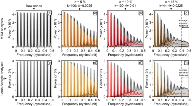
The effect of randomising the sample positions within the section is first tested on a sum of pure sinusoids. A dataset of 600 points is generated with a sample step of 1 arbitrary unit. The series is a sum of 24 sinusoids, having equal am-plitudes and different frequencies: frequencies range from 0.02 to 0.48 cycles (arbitrary unit)−1 and increase with in-crements of 0.02 cycles (arbitrary unit)−1 (Fig. 3a, b). Fig-ure 3 shows the 2π MTM and Lomb–Scargle spectra of the sum of sinusoids before and after applying 1000 Monte Carlo simulations of distorted sample distances. The grey zones in-dicate the interval covering 95 % of the power in the 1000 simulations. The average spectrum of these simulations is shown in orange for the test with 5 % stratigraphic uncer-tainty (Fig. 3c, d), red for 10 % unceruncer-tainty (Fig. 3e, f) and brown for 15 % uncertainty (Fig. 3g, h). The most striking feature after gamma-model randomisation is the progressive and strong decrease in the power spectrum towards the high frequencies, even when the lowest level of uncertainty (5 %) is considered.
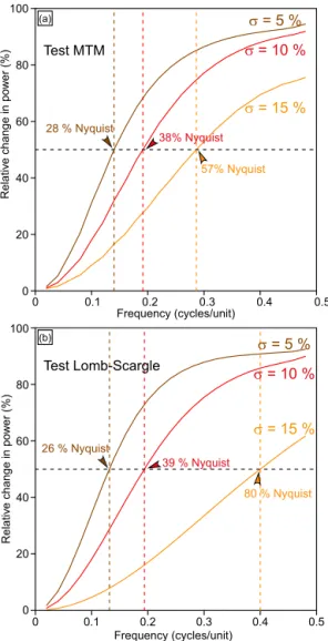
Figure 4 notably shows the relative change in power of the average spectrum after applying the 1000 simulations. At 5 %
uncertainty, a decrease of 50 % in the power spectrum is ob-served in the 2π -MTM spectrum at 57 % of the Nyquist fre-quency, equivalent to 3.5 times the average sample distance. The level of 50 % of decrease in the power spectrum is ob-served in the Lomb–Scargle spectrum at 80 % of the Nyquist frequency, i.e. 2.5 times the average sample distance. This implies that even for a very low level of noise, the values of the power spectrum can be largely underestimated in the up-per half of the spectrum. At 10 % uncertainty, a decrease of 50 % in the power spectrum is observed at 38–39 % of the Nyquist frequency, both in the Lomb–Scargle and the 2π -MTM spectra, which is equivalent to 5.2 times the average sample distance. Finally, at 15 % uncertainty, both Lomb– Scargle and 2π MTM indicate that 50 % of decrease in the power spectrum has occurred at 27 % of the Nyquist fre-quency, which is equivalent to 7.4 times the average sam-ple distance. This examsam-ple shows that the worse the control of the sample position in the sedimentary series is, the more samples per cycle one needs to limit the loss of power of the cycles targeted.
Stratigraphic uncertainty does not only trigger loss of power of the spectral peaks, it also increases the power spec-tral background (Fig. 3). At 5 and 10 % uncertainties, the average and background spectrum still preserve the struc-ture of individual peaks in both 2π MTM and Lomb–Scargle analyses (Fig. 3c–f). Indeed, spectra for individual Monte Carlo simulations still exhibit spectral peaks at these fre-quencies although they are characterised by variable power and deviations in the frequencies at which the peaks are lo-calised. However, at 15 % uncertainty, the average power in the highest frequencies is flattened and the structure of the peaks is not distinguishable anymore (Fig. 3e–h). This zone of the spectrum cannot be regarded as reliably interpretable. These analyses from a sum of pure sinusoids show that the higher the stratigraphic uncertainty is, the higher is the loss in power of the spectral peaks and the more the low frequen-cies are affected by this loss of power. At 15 % uncertainty, the spectrum is flattened in the highest frequency and can-not be interpreted in this part of the spectrum. Because of its higher-frequency resolution, the Lomb–Scargle analysis dis-plays higher spectrum background levels than the 2π -MTM analysis. It however changes the highest frequency that can be interpreted very little, even at 15 % uncertainty.
It should be noticed that in the case of pure sinusoids, the signal is only composed of pure harmonics concentrating the spectral power at specific frequencies. This implies that a small shift in the sample position triggers a strong decrease in the average power spectrum at these specific frequencies. In addition, in this theoretical example, the sample distance be-fore the randomisation procedure was strictly constant (1 ar-bitrary unit). More realistically, spectra of geological datasets are rather composed of a mixture of harmonics, narrowband and background components, and the sample distances are not strictly constant. For instance, because of variations in the sedimentation rates, the sedimentary expression of the orbital
0 0.2 0.4 0 Frequency (cycles/unit)0.1 0.3 0.5 3 2 1 4 0 0.2 0.4 Frequency (cycles/unit)0.1 0.3 0.5 0 3 2 1 4 0 0.2 0.4 Frequency (cycles/unit)0.1 0.3 0.5 0 3 2 1 4 0 0.2 0.4 Frequency (cycles/unit)0.1 0.3 0.5 0 3 2 1 4 Power (x10 -2) Power (x10 -2) Power (x10 -2) Power (x10 -2) 0 0.2 0.4
Frequency (cycles/unit)0.1 0.3 0.5 0Frequency (cycles/unit)0.1 0.2 0.3 0.4 0.5 0Frequency (cycles/unit)0.1 0.2 0.3 0.4 0.5 0Frequency (cycles/unit)0.1 0.2 0.3 0.4 0.5 0 1 2 3 0 1 2 3 0 1 2 3 0 1 2 3 Power (x10 2) Power (x10 2) Power (x10 2) Power (x10 2) (b) (c) (e) (g) (h) MTM analyses Lomb-Scargle analyses Raw series k=400; =0.0025 = 5 % (d) = 10 % k=100; =0.01 k=44; =0.0225 = 15 % Average spectrum flattened Average spectrum flattened (a) (f)
Figure 3.Effect of the gamma-law randomised sample distances on the 2π MTM and Lomb–Scargle spectra of the series of sum of pure
sinusoids. Panels (a) and (b): spectra of the series without sample step randomisation. Panels (c) and (d): spectra with 5 % of stratigraphic uncertainty. Panels (e) and (f): spectra with 10 % of stratigraphic uncertainty. Panels (g) and (h): spectra with 15 % of stratigraphic uncertainty. For each simulation shown from (c) to (h), the grey area represents the interval covering 95 % of the simulations, while the red, orange and brown curves represent the average spectrum.
cycles is not focused on specific frequencies but rather ex-pressed in ranges of frequencies (e.g. Weedon, 2003, p. 132). This can add some noise in the high frequencies and blur the spectra even more than in the case of pure sinusoids. In the following, the results of the application of the test to two ge-ological datasets are shown.
6 Application to geological datasets
6.1 Spectral analysis prior to randomisation 6.1.1 The La Charce series
Prior to performing 2π -MTM analyses, the gamma-ray se-ries was detrended using a best-fit linear regression, linearly interpolated to 0.20 m sample distance and standardised to zero average and unit variance (Fig. 5). Prior to REDFIT Lomb–Scargle analysis, the datasets (raw and randomised) were simply linearly detrended using a best-fit linear regres-sion and standardised.
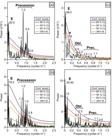
The 2π -MTM analysis of the La Charce section shows two main significant bands (> 99 % confidence level, hereafter abbreviated CL) at 20 m and from 1.3 to 0.8 m (Fig. 6a). The peak at a period of 20 m has been interpreted as the imprint of 405 kyr eccentricity forcing, while the group of peaks at 1.3 to 0.8 m has been dominantly related to precession (Boulila et al., 2015; Martinez et al., 2013, 2015). The REDFIT spec-trum shows two bands of periods exceeding the 99 % CL at
18 m and from 1.4 to 0.8 m (Fig. 6b). These periods are sim-ilar to the periods observed in the 2π -MTM spectrum. The small differences in periodicity observed in the lowest quencies are likely to be related to the difference in the fre-quency resolution between the two methods. In addition, the REDFIT spectrum as parameterised here produces narrower peaks than the multi-taper spectrum, so that the lowest fre-quencies in the REDFIT spectrum are composed of a group of narrow peaks, rather than a single broad peak observed in the 2π -MTM spectrum.
The autoregressive coefficient, a measure of the redness of the spectrum, is assessed at 0.440 in the 2π -MTM analy-sis, while it is assessed at 0.468 in the REDFIT analysis (Ta-ble 1). The S0 value, the average power of the red-noise pro-cess within the entire spectrum, is 3.54 × 10⁻⁴in the MTM analysis, while it is 0.398 in the REDFIT analysis (Table 1). This difference in the S0 value is due to the difference in signal treatment when calculating the MTM or the REDFIT spectrum.
6.1.2 The La Thure series
Prior to performing 2π -MTM analyses, the magnetic suscep-tibility series was detrended by subtracting a piecewise best-fit linear regression (Fig. 7a). The series was then linearly interpolated to a sample distance of 0.38 m, and the trend of the variance was removed by dividing the series by its in-stantaneous amplitude smoothed with a LOWESS (locally
Table 1.Results of red-noise background estimates from the La Charce and the La Thure series with the 2π MTM and the REDFIT analyses.
σ =0 % σ =5 % σ =10 % σ =15 %
La Charce MTM Autoregressive coefficient 0.440 0.433 ± 0.025 0.432 ± 0.037 0.434 ± 0.048
Average power (×10−4) 3.54 3.55 ± 0.13 3.58 ± 0.20 3.61 ± 0.25
La Charce REDFIT Autoregressive coefficient 0.468 0.468 ± 0.002 0.467 ± 0.003 0.467 ± 0.006
Average power 0.398 0.399 ± 0.003 0.402 ± 0.005 0.407 ± 0.008
La Thure MTM Autoregressive coefficient 0.657 0.658 ± 0.025 0.653 ± 0.029 0.651 ± 0.033
Average power (×10−3) 1.67 1.67 ± 0.04 1.67 ± 0.05 1.68 ± 0.07
La Thure REDFIT Autoregressive coefficient 0.407 0.406 ± 0.004 0.405 ± 0.008 0.404 ± 0.013
Average power 0.890 0.894 ± 0.011 0.900 ± 0.019 0.904 ± 0.027 0 0.1 0.2 0.3 0.4 0.5 0 20 40 60 80 100 Frequency (cycles/unit) Relativ e change in p ow er (%) (b) 0.1 0.2 0.3 0.4 0 20 40 60 80 100 Frequency (cycles/unit) Relati ve change in p ow er (%) 0 0.5 (a) 80 % Nyquist 39 % Nyquist 26 % Nyquist 57% Nyquist 38% Nyquist 28 % Nyquist Test MTM Test Lomb-Scargle σ = 5 % σ = 10 % σ = 15 % σ = 5 % σ = 10 % σ = 15 %
Figure 4. Relative change in power in the (a) 2π -MTM spectra
and (b) Lomb–Scargle spectra after applying the gamma-law simu-lations of distortion of the time series. The arrows indicate at which frequency (relatively to the Nyquist frequency) the change in power reaches 50 %. 6 8 10 12 14 0 20 40 60 80 100 Level (m)
Spectral gamma ray
(ppm eU) −2 −1 0 1 2 3
Spectral gamma ray detrended, normalised
Level (m)
0 20 40 60 80 100
(a)
(b)
Figure 5.Detrending procedure of the gamma-ray series from the
La Charce section. (a) Raw gamma-ray signal (black curve) with best-fit linear trend (red curve). (b) Gamma-ray series after subtrac-tion of the linear trend and standardisasubtrac-tion (average = 0; standard deviation = 1).
weighted scatterplot smoothing) regression with a 10 % co-efficient (Fig. 7b). Such an approach allows the series to have a stationary mean and variance (Fig. 7c). The series was sub-sequently standardised (average = 0; standard deviation = 1). Prior to the REDFIT analysis, the identical procedure was ap-plied, except for interpolation at an even sample step, as this is not required by the Lomb–Scargle method.
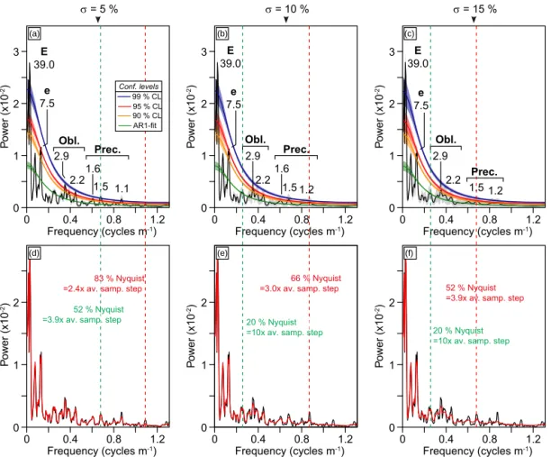
The 2π -MTM analysis of the La Thure section shows sig-nificant periods at 39 m (>99 % CL), interpreted as the mani-festation of the 405 kyr eccentricity cycle (De Vleeschouwer et al., 2015), and at 7.8 m (> 95 % CL), interpreted as 100 kyr eccentricity cycles; it also shows a group of significant peri-ods from 2.8 to 2.2 m (99 % CL), interpreted as obliquity,
0 0.5 1.0 1.5 2.0 2.5 0 2 4 6 Frequency (cycles m )-1 Po w er (x10 -3) 0 0.2 0.4 0.6 0.8 1.0 1.2 0 1 2 3 Frequency (cycles m )-1 Po w er (x10 -2) 0 0.5 1.0 1.5 2.0 2.5 0 1 2 3 4 5 6 Frequency (cycles m-1) Power 0 0.2 0.4 0.6 0.8 1.0 1.2 0 5 10 15 Frequency (cycles m )-1 Power E 20.5 1.3 1.2 0.9 0.8 Precession E 18.2 1.3 1.2 1.0 0.8 Precession E 39.0 e 7.8 2.9 2.2 Obl. 1.6 1.5 1.1 Prec. E 30-40 3.32.3 13 Obl. (a) (c) (b) (d) 1.1 1.5 0.9 Prec. Conf. levels 99 % CL 95 % CL 90 % CL AR1-fit Conf. levels 99 % CL 95 % CL 90 % CL AR1-fit Conf. levels 99 % CL 95 % CL 90 % CL AR1-fit Conf. levels 99 % CL 95 % CL 90 % CL AR1-fit
Figure 6.Spectra of the La Charce and La Thure series before
Monte Carlo simulations of the sample distances. (a) 2π -MTM spectrum of the La Charce series. (b) REDFIT spectrum of the La Charce series. (c) 2π -MTM spectrum of the La Thure series. (d) REDFIT spectrum of the La Thure series. The main significant periods are given in metres.
and a group of significant periods from 1.6 to 1.1 m (> 95 and > 99 % CL), interpreted as precession (Fig. 6c). In the lowest frequencies, the REDFIT spectrum (Fig. 4f) shows a group of peaks centred on 30–40 m (> 99 % CL) and a peak at 13 m (> 95 % CL), which is not significant in the 2π -MTM spectrum. Conversely, the period at 7.9 m observed in the 2π -MTM spectrum does not reach the 90 % CL in the REDFIT spectrum. These differences are likely related to the difference in frequency resolution between both meth-ods and to the fact that REDFIT spectra as parameterised here produce narrower peaks than the 2π -MTM spectra. In the REDFIT spectrum, the obliquity band shows two periods at 3.3 m (95 % CL) and 2.3 m (> 95 % CL). The precession band shows periods at 1.5 m (> 90 % CL), 1.1 m (> 99 % CL) and at 0.9 m (> 95 % CL).
The autoregressive coefficient of the red-noise background level is assessed at 0.657 in the 2π -MTM analysis and at 0.407 in the REDFIT analysis (Table 1). The difference in the autoregressive coefficient is due to the method of calculating the red-noise background (from the spectrum in the MTM analysis and from the time series in the REDFIT analysis; Mann and Lees, 1996; Meyers, 2014; Mudelsee, 2002). The
0 50 100 150 0 1 2 3 Level (m) MS (x10 m kg ) -7 3 0 50 100 150 -5 5 Level (m) 0 50 100 150 -2 -1 0 1 2 3 Level (m) MS average-detrended (x10 m kg ) -8 3 -1 0 10 15 MS variance-detrended, normalised (a) (b) (c) -1
Figure 7. Detrending procedure of the magnetic susceptibility
(MS) series from the La Thure section. (a) Raw MS signal (black curve) with piecewise best-fit linear trend of the average (red curve). (b) MS series after subtraction of the piecewise linear trend (black curve), with instantaneous amplitude (green curve) and LOWESS regression of the instantaneous amplitude applied with a coeffi-cient of 10 % (red curve). (c) MS curve after dividing the MS se-ries “average-detrended” by the LOWESS regression of the instan-taneous amplitude and after standardisation.
Lomb–Scargle analysis also tends to produce higher pow-ers in the high frequencies, thus reducing the autoregres-sive coefficient estimate in the REDFIT analysis (Schulz and Mudelsee, 2002). This difference also illustrates the diffi-culty in calculating the autoregressive coefficient when the redness of the spectrum increases (see Meyers, 2012). Fi-nally, the S0 value is assessed at 1.67×10⁻³in the 2π -MTM analysis and at 0.890 in the REDFIT analysis (Table 1).
6.2 Impact on the power spectrum of randomising the sample distances
6.2.1 The La Charce series
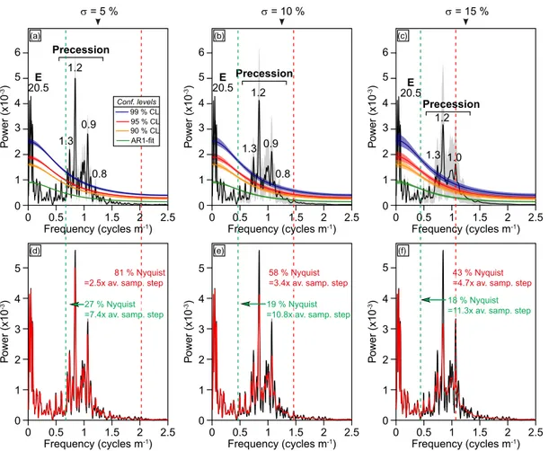
At 5 % uncertainty, the average 2π -MTM spectrum of the La Charce still shows periods at 20.5 m as well as several pe-riods around 1 m exceeding the 99 % CL (Fig. 8a). At 10 % uncertainty, the peak at 0.8 m does not exceed the 95 % CL (Fig. 8b), and it is completely smoothed at 15 % uncertainty (Fig. 8c). The increasing level of stratigraphic uncertainty
Table 2.Synthesis of the results of highest frequencies before smoothing of the spectra when applying the Monte Carlo simulations and of highest frequency at which the spectra before and after simulation are practically identical.
Level of stratigraphic uncertainty
σ =5 % σ =10 % σ =15 %
La Charce MTM
Highest frequency before smoothing 81 % Nyquist 58 % Nyquist 43 % Nyquist
Equivalent number sample steps 2.5× 3.4× 4.7×
Highest-frequency confounded spectra 27 % Nyquist 19 % Nyquist 18 % Nyquist
Equivalent number sample steps 7.4× 10.8× 11.3×
La Charce REDFIT
Highest frequency before smoothing 58 % Nyquist 42 % Nyquist
Equivalent number sample steps 3.4× 4.8×
Highest-frequency confounded spectra 28 % Nyquist 18 % Nyquist 18 % Nyquist
Equivalent number sample steps 6.8× 10.9× 10.9×
La Thure MTM
Highest frequency before smoothing 83 % Nyquist 66 % Nyquist 52 % Nyquist
Equivalent number sample steps 2.4× 3.0× 3.9×
Highest-frequency confounded spectra 52 % Nyquist 20 % Nyquist 20 % Nyquist
Equivalent number sample steps 3.9× 10× 10×
La Thure REDFIT
Highest frequency before smoothing 53 % Nyquist 53 % Nyquist
Equivalent number sample steps 3.8× 3.8×
Highest-frequency confounded spectra 52 % Nyquist 22 % Nyquist 20 % Nyquist
Equivalent number sample steps 3.9× 9.3× 10×
progressively smooths the average spectrum, with the high-est frequencies most affected (Fig. 8d–f). Notably at 5 % un-certainty, fluctuations of the spectrum at frequencies higher than 81 % of the Nyquist frequency are suppressed (Table 2). At 10 and 15 % uncertainty, this threshold decreases to re-spectively 58 and 43 % of the Nyquist frequency (Fig. 8d–f). Increasing levels of uncertainty also tend to reduce the power of the spectral peaks in an increasing portion of the spectrum. At 5 % uncertainty, the average spectrum of the simulations is practically identical to the spectrum of the original series from frequency 0 to 27 % of the Nyquist frequency (Fig. 8d). This range is reduced to 0–19 % of the Nyquist frequency at 10 % uncertainty (Fig. 8e) and to 0–18 % of the Nyquist frequency at 15 % uncertainty (Fig. 8f).
In the REDFIT spectrum with 5 % of stratigraphic uncer-tainty, the periods at 20.5 m and around 1 m still exceed the 99 % CL (Fig. 9a). Like in the 2π -MTM analyses, the pe-riod at 0.8 m does not exceed the 99 % CL at 10 % uncer-tainty, while it is completely smoothed at 15 % uncertainty (Fig. 9b–c). The tendency of the Lomb–Scargle analysis to produce high-power peaks in the high frequencies limits the effect of the smoothing of the spectrum at 5 % uncertainty (Fig. 9d). However, at 10 and 15 % uncertainties, fluctuations in the spectrum at frequencies higher than respectively 58 and 42 % of the Nyquist frequency are completely smoothed (Fig. 9e–f; Table 2). At 5 % uncertainty, the average spec-trum of the simulations cannot be distinguished from the spectrum of the original series from frequency 0 to 29 % of
the Nyquist frequency (Fig. 9d), while at 10 and 15 % un-certainties, this range is restricted to 0–19 % of the Nyquist frequency (Fig. 9e–f).
The average autoregressive coefficients of the 1000 simu-lations (with ± the interval covering 95 % of the simusimu-lations) are assessed for 5, 10 and 15 % of stratigraphic uncertain-ties at 0.433 ± 0.025, 0.432 ± 0.037 and 0.434 ± 0.048 re-spectively in the 2π -MTM analyses and at 0.468 ± 0.002, 0.467 ± 0.003 and 0.467 ± 0.006 respectively in the RED-FIT analyses (Table 1). The average S0 values of the 1000 simulations are assessed for 5, 10 and 15 % of stratigraphic uncertainties at 3.55 × 10⁻⁴±0.13 × 10⁻⁴, 3.58 × 10⁻⁴± 0.20 × 10⁻⁴and 3.61 × 10⁻⁴±0.25 × 10⁻⁴respectively in the 2π -MTM analyses and at 0.399 ± 0.003, 0.402 ± 0.005 and 0.407 ± 0.008 respectively in the REDFIT analyses.
6.2.2 The La Thure series
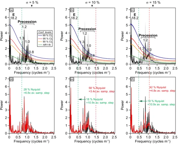
At 5 % uncertainty, the 2π -MTM spectrum of the La Thure series still exhibits significant frequencies at 39, 1.5 and 1.1 m exceeding the 99 % CL and at 7.5, 2.9, 2.2 and 1.6 m exceeding the 95 % CL (Fig. 10a). At 10 % uncertainty, the 1.1 m peak is much smoother, centred on a period of 1.2 m and only exceeds the 95 % CL (Fig. 10b). The other periods of the precession, at 1.5 and 1.6 m, only exceed the 90 and 95 % CL respectively. The significant periods of the obliq-uity bands, at 2.2 and 2.9 m, show weaker powers than in the spectrum of the original series but still exceed the 95 % CL. At 15 % uncertainty, the band of periods at 1.2 m is nearly
0 2 4 6 Po w er (x10 -3) 0 0.5 1.5 2 2.5
Frequency (cycles m )1 -1 0 Frequency (cycles m )0.5 1 1.5 2-1 2.5 0 Frequency (cycles m )0.5 1 1.5 2-1 2.5
0 0.5 1.5 2 2.5
Frequency (cycles m )1 -1 0 Frequency (cycles m )0.5 1 1.5 2-1 2.5 0 Frequency (cycles m )0.5 1 1.5 2-1 2.5 0 2 4 6 Po w er (x10 -3) 0 2 4 6 Po w er (x10 -3) 0 2 4 Po w er (x10 -3) 1 3 5 0 2 4 Po w er (x10 -3) 1 3 5 0 2 4 Po w er (x10 -3) 1 3 5 1 3 5 1 3 5 1 3 5 E 20.5 1.3 1.2 0.9 0.8 Precession (a) (b) (c) (d) (e) (f) E 20.5 1.3 1.2 0.9 0.8 Precession E 20.5 1.3 1.2 1.0 Precession 81 % Nyquist
=2.5x av. samp. step 58 % Nyquist=3.4x av. samp. step 43 % Nyquist=4.7x av. samp. step 27 % Nyquist
=7.4x av. samp. step 19 % Nyquist=10.8x av. samp. step
18 % Nyquist =11.3x av. samp. step
σ = 5 % σ = 10 % σ = 15 % 95 % CL 90 % CL AR1-fit Conf. levels 99 % CL
Figure 8.Effect of the gamma-law randomisation of the sample distances on the 2π -MTM spectrum of the La Charce series. Panels a to
c: 2π -MTM spectra with a level of stratigraphic uncertainty fixed to 5, 10 and 15 % of the average sample distance of the series. The grey area represents the interval covering 95 % of the simulations. The average confidence levels are reported on the spectra with their respective areas covering 95 % of the simulations. Main significant periods are indicated in metres with, in bold, their corresponding orbital cycles. E: 405 kyr eccentricity. Panels d to f: superposition of the 2π -MTM spectra before randomisation (in black) and the average spectrum after the 1000 simulations (in red). The red dashed lines indicate the lowest frequency above which the spectrum is completely smoothed, so that no other frequency can be identified. The green dashed lines represent the highest frequency below which the spectrum of the series before randomisation appears practically identical to the spectrum after randomisation.
entirely flattened and hardly distinguishable from the spec-tral background (Fig. 10c). In addition, all frequencies from the obliquity and the precession do not exceed the 95 % CL. The reduction in the significance levels in the precession and obliquity bands is the consequence of increasing loss in power of the spectral peaks at high frequencies. At 5 % uncertainty, the average spectrum of the simulations is prac-tically identical to the spectrum of the original series from frequency 0 to 52 % of the Nyquist frequency (Fig. 10d), while at 10 and 15 % uncertainties, this range is restricted to 0–20 % of the Nyquist frequency (Fig. 10e–f; Table 2).
At 5 % uncertainty, the REDFIT analysis still displays sig-nificant periods at 30–40 m exceeding the 99 % CL and a pe-riod at 2.3 m exceeding the 95 % CL (Fig. 11a). The peak at 1.5 m does not exceed the 90 % CL anymore, while the peaks at 1.1 and 0.9 m do not exceed the 95 % CL anymore. At 10 % uncertainty and 15 % uncertainties, spectral peaks in
the precession and the obliquity bands do not reach the 95 % CL anymore. The tendency of the Lomb–Scargle analysis to produce high-power peaks in the high frequencies prevents strong smoothing of the power spectrum at 5 % uncertainty. However, at 10 and 15 % uncertainties, all fluctuations of the power spectrum at frequencies higher than 53 % Nyquist fre-quency are flattened and not distinguishable (Table 2). The significance level in the eccentricity band is still preserved in the average spectrum. At 10 and 15 % uncertainty, the power spectrum displays spectral peaks with reduced powers com-pared to the spectrum of the original series, which impacts the significance levels in the obliquity and precession bands (Fig. 11d–f). At 5 % uncertainty the REDFIT spectrum of the La Thure series remains practically unchanged compared to the spectrum of the original series from 0 to 58 % Nyquist frequency (Fig. 11d), while at 10 and 15 % uncertainty this
0 0.5 1.0 1.5 2.0 2.5 0 1 2 3 4 5 6 7 Frequency (cycles m-1) Po w er 0 0.5 1.0 1.5 2.0 2.5 Frequency (cycles m )-1 Po w er 0 0.5 1.0 1.5 2.0 2.5 Frequency (cycles m )-1 Po w er 0 0.5 1.0 1.5 2.0 2.5 0 1 2 3 4 5 6 7 Frequency (cycles m-1) Po w er 0 0.5 1.0 1.5 2.0 2.5 Frequency (cycles m )-1 Po w er 0 0.5 1.0 1.5 2.0 2.5 Frequency (cycles m )-1 Po w er 0 1 2 3 4 5 6 7 0 1 2 3 4 5 6 7 0 1 2 3 4 5 6 7 0 1 2 3 4 5 6 7 E 18.2 1.3 1.2 1.0 0.8 Precession E 18.2 1.3 1.2 1.0 0.8 Precession E 18.2 1.3 1.2 1.0 Precession (a) (b) (c) (d) (e) 58 % Nyquist
=3.4x av. samp. step 42 % Nyquist=4.8x av. samp. step 18 % Nyquist
=10.9x av. samp. step 18 % Nyquist=10.9x av. samp. step 28 % Nyquist
=6.8x av. samp. step
95 % CL 90 % CL AR1-fit Conf. levels 99 % CL σ = 5 % σ = 10 % σ = 15 % (f)
Figure 9.Effect of the gamma-law randomisation of the sample distances on the REDFIT spectrum of the La Charce series. Panels a to
c: REDFIT spectra with a level of stratigraphic uncertainty fixed to 5, 10 and 15 % of the average sample distance of the series. The grey area represents the interval covering 95 % of the simulations. The average confidence levels are reported on the spectra with their respective areas covering 95 % of the simulations. Main significant periods are indicated in metres with, in bold, their corresponding orbital cycles. E: 405 kyr eccentricity. Panels d to f: superposition of the REDFIT spectra before randomisation (in black) and the average spectrum after the 1000 simulations (in red). The red dashed lines indicate the lowest frequency above which the spectrum is completely smoothed, so that no other frequency can be identified. The green dashed lines represent the highest frequency below which the spectrum of the series before randomisation appears practically identical to the spectrum after randomisation.
range is respectively restricted to 0–22 and 0–19 % Nyquist frequency (Fig. 11e–f).
The average autoregressive coefficients of the 1000 simu-lations are assessed for 5, 10 and 15 % of stratigraphic uncer-tainties at 0.658 ± 0.025, 0.653 ± 0.029 and 0.651 ± 0.033 respectively in the 2π -MTM analyses and at 0.406 ± 0.004, 0.405 ± 0.008 and 0.404 ± 0.013 respectively in the RED-FIT analyses (Table 1). The average S0 values of the 1000 simulations are assessed for 5, 10 and 15 % of stratigraphic uncertainties at 1.67 × 10⁻³±0.04 × 10⁻³, 1.67 × 10⁻³± 0.05 × 10⁻³and 1.68 × 10⁻³±0.07 × 10⁻³ respectively in the 2π -MTM analyses and at 0.894 ± 0.011, 0.900 ± 0.019 and 0.904 ± 0.008 respectively in the REDFIT analyses.
7 Discussion
7.1 Comparison of the results between the two geological datasets
In the 2π -MTM simulations, the spectral peaks tend to be smoothed at 5 % of stratigraphic uncertainty from ∼ 80 % Nyquist frequency to the Nyquist frequency, which implies that taking at least three samples per cycle of interest should not smooth the spectral peaks in the frequency band targeted (e.g. the Milankovitch cycles; Table 2). In the REDFIT simu-lations, the tendency of the spectrum to produce high-power spectra in high frequencies even makes all the spectral peaks of the original spectrum still identifiable at 5 % uncertainty. If a low level of stratigraphic uncertainty is maintained, prac-tically all spectral peaks at frequencies below 80 % Nyquist frequencies will be preserved. These thresholds dramatically decrease to 53 to 66 % of Nyquist frequencies at 10 % of
0 0.4 0.8 1.2 0 1 2 3 Frequency (cycles m-1) 0 0.4 0.8 1.2 0 1 2 3 Frequency (cycles m-1) 0 0.4 0.8 1.2 0 1 2 3 Frequency (cycles m-1) 0 1 2 0 1 2 0 1 2 0 0.4 0.8 1.2
Frequency (cycles m )-1 0 Frequency (cycles m )0.4 0.8 -11.2 0 Frequency (cycles m )0.4 0.8 -11.2 2.9 2.21.61.5 1.1 Obl. Prec. 2.9 2.21.6 1.5 1.2 Obl. Prec. 2.9 2.2 1.5 1.2 Obl. Prec. (a) (b) (c) (d) (e) (f) 52 % Nyquist =3.9x av. samp. step
Po w er (x10 -2) Po w er (x10 -2) Po w er (x10 -2) Po w er (x10 -2) Po w er (x10 -2) Po w er (x10 -2) E 39.0 39.0E 39.0E e 7.5 7.5e 7.5e 83 % Nyquist =2.4x av. samp. step
52 % Nyquist
=3.9x av. samp. step 20 % Nyquist
=10x av. samp. step 66 % Nyquist =3.0x av. samp. step
20 % Nyquist =10x av. samp. step
σ = 5 % σ = 10 % σ = 15 % 95 % CL 90 % CL AR1-fit Conf. levels 99 % CL
Figure 10.Effect of the gamma-law randomisation of the sample distances on the 2π -MTM spectrum of the La Thure series. Panels a to c:
2π -MTM spectra with a level of stratigraphic uncertainty fixed to 5, 10 and 15 % of the average sample distance of the series. The grey area represents the interval covering 95 % of the simulations. The average confidence levels are reported on the spectra with their respective areas covering 95 % of the simulations. Main significant periods are indicated in metres with, in bold, their corresponding orbital cycles. E: 405 kyr eccentricity; e: 100 kyr eccentricity. Panels d to f: superposition of the 2π -MTM spectra before randomisation (in black) and the average spectrum after the 1000 simulations (in red). The red dashed lines indicate the lowest frequency above which the spectrum is completely smoothed, so that no other frequency can be identified. The green dashed lines represent the highest frequency below which the spectrum of the series before randomisation appears practically identical to the spectrum after randomisation.
stratigraphic uncertainty in all simulations, while it decreases to 42 to 53 % of Nyquist frequency at 15 % uncertainty. Thus, a medium level of stratigraphic uncertainty implies taking at least four samples per cycles of interest, while a high level of uncertainty implies taking at least five samples per cycle of interest.
Comparisons between original and average simulated spectra show that at 5 % uncertainty, both are practically identical from 0 to 27 % of Nyquist frequency in the La Charce series and from 0 to 52 % of Nyquist frequency in the La Thure series. At 10 and 15 % uncertainties, these ranges dramatically shift from 0 to 20–22 % Nyquist frequency. Al-though differences exist in the variance of the average spec-trum and in the frequency resolution between the 2π MTM and the REDFIT analyses, both analyses show, for each se-ries, the same range of frequencies in which simulated and original spectra are identical. These thresholds imply that
taking four to eight samples per cycle of interest should limit the loss of power of the spectral peaks in the targeted bands at 5 % uncertainty. At 10 and 15 % uncertainty, taking at least 10 samples per cycle of interest should limit the loss of power in the targeted band. Limiting the loss of power in the frequencies of interest appears to be crucial because the average power of the confidence levels remain unchanged after applying the simulations. Simulations of distortions of the geological series smooths the spectrum by distributing the power spectrum from the spectral peaks to the surround-ing frequencies. The calculation of confidence levels in the MTM analyses is based on a moving median of the power spectrum performed over a broad range of frequencies (usu-ally one fifth of the total spectrum; Mann and Lees, 1996). Thus, when distorting the time series, the distribution of the power spectrum over a narrow range of frequencies does not change the overall median of the power spectrum calculated
0 0.4 0.8 1.2 0 2 4 6 8 10 12 Frequency (cycles m-1) Po w er 0 0.4 0.8 1.2
Frequency (cycles m )-1 0 Frequency (cycles m )0.4 0.8 -11.2
0 2 4 6 8 10 Po w er 0 0.4 0.8 1.2
Frequency (cycles m )-1 0 Frequency (cycles m )0.4 0.8 -11.2 0 Frequency (cycles m )0.4 0.8 -11.2 0 2 4 6 8 10 12 Po w er 0 2 4 6 8 10 Po w er 0 2 4 6 8 10 12 Po w er 0 2 4 6 8 10 Po w er (a) (b) (c) (d) (e) (f) E 30-40 13 3.32.3 Obl. 1.5 1.1 0.9Prec. E 30-40 13 3.32.3 Obl. E 30-40 13 3.32.3 Obl. 1.5 1.5 Prec. Prec. 52 % Nyquist =3.9x av. samp. step
53 % Nyquist =3.8x av. samp. step
22 % Nyquist
=9.3x av. samp. step 20 % Nyquist=10x av. samp. step
53 % Nyquist =3.8x av. samp. step
95 % CL 90 % CL AR1-fit Conf. levels 99 % CL σ = 5 % σ = 10 % σ = 15 %
Figure 11.Effect of the gamma-law randomisation of the sample distances on the REDFIT spectrum of the La Charce series. Panels a to c:
REDFIT spectra with a level of stratigraphic uncertainty fixed to 5, 10 and 15 % of the average sample distance of the series. The grey area represents the interval covering 95 % of the simulations. The average confidence levels are reported on the spectra with their respective areas covering 95 % of the simulations. Main significant periods are indicated in metres with, in bold, their corresponding orbital cycles. E: 405 kyr eccentricity; e: 100 kyr eccentricity. Panels d to f: superposition of the REDFIT spectra before randomisation (in black) and the average spectrum after the 1000 simulations (in red). The red dashed lines indicate the lowest frequency above which the spectrum is completely smoothed, so that no other frequency can be identified. The green dashed lines represent the highest frequency below which the spectrum of the series before randomisation appears practically identical to the spectrum after randomisation.
over one fifth of the total spectrum and thus does not change the average level of confidence levels after simulations. The effect of time-series distortions on the power of confidence levels is even smaller in the REDFIT analysis, in which the confidence levels are directly calculated on the time series it-self and not on the spectrum (Mudelsee, 2002). The decrease in the power of the spectral peaks due to distortions of the geological series thus implies a decrease in the significance levels of the main cycles of the series. In the case of a low level of red noise, like in the La Charce series (Figs. 8–9), spectral smoothing and decrease in power in the precession band does not strongly impact the interpretations, since the significance level in the precession band still exceed the 99 % CL, even after the implementation of a level of 15 % of strati-graphic uncertainty. However, in the case of strong red noise, like in the La Thure series, the decrease in power at high fre-quencies has a strong impact on the significance levels after
the implementation of the simulations. At a medium level of stratigraphic uncertainty (10 %), taking 10 samples per cycle of interest is needed to limit the loss of power in the cycles of interest and thus to limit the decrease in the level of sig-nificance of these targeted cycles.
As an example, if the targeted range of frequencies are the Milankovitch cycles, the shortest period of interest is the pre-cession cycles. A density of one sample per 4 kyr should al-low the detection of the spectral peaks in the precession band. A density of sampling of one sample per 2 kyr should then ensure the detection of significant peaks in the precession band, even in the case of strong red noise and medium-to-high levels of stratigraphic uncertainty. The minimum den-sity of sampling being dependant on the level of red noise and stratigraphic uncertainty, we strongly recommend apply-ing the simulations developed here to assess the impact of
stratigraphic uncertainty on the identification of significant spectral peaks in the sedimentary record.
7.2 In which case should this test be applied?
Uncertainties in the measurement of sample position can practically not be avoided in outcrop conditions. The sim-ilarity between the topographic slope and the sedimentary dip, the absence or scarcity of marker beds, or the need to move laterally in a section can trigger disturbances in the sampling regularity. In core sedimentary sequences, non-destructive automated measurements such as X-ray fluores-cence, gamma-ray spectrometry or magnetic susceptibility should limit errors in the sample position. However, physi-cal samplings (e.g. for geochemistry or mineralogy) are sub-ject to small uncertainties, especially when the sampling res-olution is very high. Core sedimentary series can in addition be affected by the expansion of sediment caused by the re-lease of gas or the rere-lease of overburden pressure (Hagelberg et al., 1995). This test is thus useful for geologists who wish to run spectral analyses on sedimentary depth series gener-ated from outcropping sections or core samples. All analyses in this paper show that with higher uncertainty in the sample step, the low frequencies are increasingly affected. The rel-ative change in power between the various tests all showed different patterns, and no general model could be deduced. The relative change in power at a given frequency depends on the dispersion of the sample step, on the method of spectral analysis and on the original sedimentary sequence studied. Each depth series generated from this sampling can be seen as one of the 1000 random simulations. The test randomises the sample position from the original series and produces a smooth version of the spectrum of the raw series. The gener-ation of the raw series impacts on the test at frequencies with low powers (a small change in a weak power can trigger high values of relative change in power) and at high frequencies. The relative change in power does not depend on the size of the sample step itself, as the same proportion of the spectrum is affected for a given level of uncertainty. However, a con-trol on the dispersion of the sample steps and the application of the test proposed here are needed to assess the dispersion of the sample distances during the sampling procedure and the impact of this dispersion on the spectrum. The question is how to assess the dispersion of the sample step in the field. If the section is well bedded, we suggest applying the same procedure as we did for La Charce, i.e. sample position mea-sured independently of the bed thickness measurements and precise reporting of the sample positions in the sedimentary log of the series. Orbital forcing can also be detected in a monotonous thick marly section, showing no apparent bed-ding (e.g. Ghirardi et al., 2014; Matys Grygar et al., 2014). In that case, we instead suggest measuring the total thickness of the sequence several times to assess the potential dispersion of the sample steps.
7.3 Implications for astronomical timescale and palaeoclimate reconstructions
Linking sedimentary cycles to orbital cycles or assessing the quality of an orbital tuning procedure often requires a good matching between the sedimentary period ratios and the or-bital period ratios (Huang et al., 1993; Martinez et al., 2012; Meyers and Sageman, 2007) and/or the determination of the amplitude modulation of the orbital cycles (Meyers, 2015; Moiroud et al., 2012; Zeeden et al., 2015). On average, strati-graphic uncertainties trigger a decrease in the power spec-trum of the main significant frequencies while distributing the power spectrum to the surrounding frequencies. In the studied geological data, stratigraphic uncertainties mostly impact the precession band, by decreasing the power and significance levels of the spectral peaks and multiplying the main frequencies for each individual runs. The occurrence of low-power spectral peaks in the precession bands and the fact that frequency ratios between the precession and lower fre-quencies do not match the orbital frequency ratios are quite common in geological data (e.g. Ghirardi et al., 2014; Huang et al., 2010; Thibault et al., 2016) and can be a consequence of stratigraphic uncertainties. Variations in the sedimentation rate produce a similar effect to stratigraphic uncertainties and can be modelled with the Monte Carlo simulations ap-plied in this study. As sedimentation rates always vary within a sedimentary series, any particular astronomical cycle can be recorded on various thicknesses of sediments, which in turn decreases the power of this astronomical cycle and dis-tributes its power over a large range of frequencies (Weedon, 2003). Stratigraphic uncertainties thus add additional noise which blurs the spectra of sedimentary series at high frequen-cies. Astronomical tuning can help in removing the effects of stratigraphic uncertainties and variations in sedimentation rates (e.g. Hays et al., 1976; Huang et al., 2010; Zeeden et al., 2013). The identification of the repetition of any astronomi-cal cycle and their attribution to the same duration removes the effects of distortion of the sedimentary series and con-centrates the variance of the power over several frequencies. Filtering a band of frequencies of interest can help in iden-tifying the repetition of the cycle used for the astronomical calibration (e.g. Westerhold et al., 2008; Thibault et al., 2016; De Vleeschouwer et al., 2015). Because of distortions of the sedimentary series, a filter, if designed very narrowly, can lead to a distortion of the actual amplitude and number of repetitions of the filtered frequency. This is particularly crit-ical for the precession band, which has been proven to be sensitive to stratigraphic uncertainty (Figs. 8 to 11) and for which amplitude modulation is governed by eccentricity. The use of a wideband filter, such as in the procedure of Zeeden et al. (2015), limits these biases and helps in a better struction of the short wavelengths. Otherwise, a robust recon-struction of the amplitude modulation of the precession band requires limited biases of the power spectrum in the preces-sion, which requires a good control on the sample position in
the field. In addition, the simulations indicate that taking at least 4–10 samples per cycle should allow the calculation of robust power spectra estimates in the respective cycle band (Table 1; Figs. 8–11).
Also in the evaluation of the relative contribution of pre-cession and obliquity-related climatic forcing, an accurate assessment of the respective spectral power is essential (Ghi-rardi et al., 2014; Latta et al., 2006; Martinez et al., 2013; Weedon et al., 2004). Notably, whenever obliquity cycles are expressed more strongly compared to precession cycles, this has been interpreted as a reflection of important climate dy-namics and feedback mechanisms at high latitudes (Ruddi-man and McIntyre, 1984), the build-up and decay of quasi-stable carbon reservoirs (Laurin et al., 2015), or direct obliq-uity forcing at tropical latitudes (Bosmans et al., 2015; Park and Oglesby, 1991). A robust evaluation of the relative con-tribution of precession and obliquity requires at least that no bias occurs from the generation of the depth series, which includes the sampling procedure. This is particularly crucial in the case in which the autoregressive coefficient of the red-noise background is high as in the La Thure series. Because of their low powers in the spectrum of the raw series, the spectral peaks related to the precession cycles become not significant at 10 to 15 % uncertainties (Figs. 9–10). In that case, one can mistakenly interpret the absence of the record of the precession cycles in the sedimentary series, while the absence of significant high frequencies can simply be the consequence of spectral smoothing when increasing the level of stratigraphic uncertainty. Once again, a good control of the sample position accompanied by a high density of sampling will significantly improve interpretations of the relative con-tributions of the precession and obliquity to the spectrum, which will in turn help make accurate palaeoclimatic inter-pretations.
8 Conclusions
Errors made during the measurement of the stratigraphic po-sition of a sample significantly affect the power spectrum of depth series. We present a method to assess the impact of such errors that is compatible with different techniques for spectral analysis. Our method is based on a Monte Carlo pro-cedure that randomises the sample steps of the time series, using a gamma distribution. Such a distribution preserves the stratigraphic order of samples and allows controlling the av-erage and the variance of the distribution of sample steps after randomisation. The simulations presented in this pa-per show that the gamma distribution of sample steps real-istically simulates errors that are generally made during the measurement of sample positions. The three case studies pre-sented in this paper all show a strong decrease in the power spectrum at high frequencies. Simulations indicate that the power spectrum can be completely smoothed for periods less than 3–4 times the average sample distance. Thus, taking at
least three to four samples per thinnest cycle of interest (e.g. precession cycles for the Milankovitch band) should preserve spectral peaks of this cycle. However, the decrease in power observed in a large portion of the spectrum implies a decrease in the significance level of the spectral peaks. Taking at least 4–10 samples per thinnest cycle of interest should allow their significance level to be preserved, depending on the level of stratigraphic uncertainty and depending on the redness of the power spectrum. Robust reconstruction of the power spec-trum in the entire Milankovitch band requires a robust control of the sample step in the field and requires a high density of sampling. To avoid any dispersion of the power spectrum in the precession band, taking 10 samples per precession cycles appears to be a safe density of sampling. For lower-resolution sampling, we recommend applying gamma-law simulations to ensure that stratigraphic uncertainty only has limited im-pact on the spectral power and significance level of the tar-geted cycles. Gamma-law simulations can also be used to simulate the effect of variations in the sedimentation rate on insolation series, which should help in modelling the transfer from insolation series to sedimentary series.
9 Data availability
Data used in this study are available via the follow-ing links: http://www.sciencedirect.com/science/article/pii/ S0031018213000977 (Martinez et al., 2013) https://doi. pangaea.de/10.1594/PANGAEA.855764 (De Vleeschouwer et al., 2015).
Appendix A: Optimised linear interpolation
When interpolating an unevenly sampled time series to an even sample distance, part of the amplitude is lost in the high frequencies because the sample positions in the interpolated series do not necessarily correspond to the position of the maxima and minima of the original time series (Fig. A1a and b). Oversampling has been suggested to limit the loss of amplitude during the interpolation process (Hinnov et al., 2002). However, oversampling impacts the autoregressive coefficient when estimating the level of red noise in the spec-trum background (Hinnov, 2016). The optimised linear inter-polation used here is designed to limit the loss of amplitude of high-frequency cycles by finding the best-fit between the original and the resampled time series (Fig. A1c, Eq. A1):
M = 1 n·
n
X
i=1
|sori[i] − sinterp[i]|, (A1)
where M is the average misfit between the variable values of the two curves, n is the number of points compared, soriis the
original signal, and sinterpis the resampled signal at the
aver-age sample distance of the original series. This comparison is only possible if the depths (or ages) of sori[i]and sinterp[i]are
the same. This is of course not the case between the original and the resampled time series (Fig. A1b), otherwise interpo-lation would not be necessary. To circumvent this problem, the original and the resampled time series are both linearly interpolated with a sample step equal to the maximum resolu-tion by which the depths (or ages) are provided. For instance, in the case of the La Thure series, the depths are given with a resolution of 0.01 m, so that soriand sinterpare linearly
inter-polated at 0.01 m. This procedure does not change the shape of the original time series or the time series resampled at the average sample distance (Fig. A1c).
To test which resampled time series fits best with the orig-inal time series, various depths are tested as starting points to resample the time at the average sample distance (Fig. A1d). The various scenarios of starting points tested increase by dx and have the following range:
Tst.test=Tst.ori:dx : (Tst.ori+dmoy − dx), (A2)
with Tst.test being the tested starting points of time series
re-sampled at the average sample distance, Tst.oribeing the
start-ing point of the original time series, dmoy bestart-ing the average sample distance of the original time series and dx being the resolution with which the depths (or ages) are given.
The best-fit curve is the one for which M is minimised. An example of application is shown for the La Thure sec-tion in Fig. A2. Differences in the resulting spectrum be-tween the best-fit and the worst-fit resampled time series are displayed in this figure. Main differences in the spectra of the two cases are observed in the middle and high frequencies. Compared to the worst-fit resampling, the spectra of the best-fit resampling show decreased power and confidence levels
0 5 10 15 20 0 5 10 15 Level (m) MS (x10 m kg ) -8 3 -1 (a) Original time series
Resampled time series
0 0.5 1.0 1.5 2.0 0 0.5 1.0 1.5 2.0 Level (m) Level (m) 5 10 15 MS (x10 m kg ) -8 3 -1 5 10 15 MS (x10 m kg ) -8 3 -1 5 10 15 MS (x10 m kg ) -8 3 -1 0 0.5 1.0 1.5 2.0 Level (m) (b) (c) (d) Absolute difference between the original and the resampled time series Step 1: The original time series is linearly
interpolated at the average sample step of the original time series.
Step 2: Both time series are resampled
at the maximum precision of the depths (here 0.01 m) and the average absolute misfit between the two curves is calculated.
Step 3: New linear interpolation at the average
sample step are tested for various starting points. The time series for which the average misfit is minimised is regarded as the best-fit curve.
Figure A1.Scheme of the procedure of the optimised linear
inter-polation of time series.
in the middle frequencies (from 0.2 to 0.7 cycles m−1), while increased power and confidence levels occur in the high fre-quencies (from 0.7 cycles m−1to the Nyquist frequency). Fit-ting the best curve to the original time series thus impacts on the calculation of the power spectrum and the confidence lev-els of the spectral peaks.
0 0.2 0.4 0.6 0.8 1.0 1.2 0 1 2 3 4 5 Frequency (cycles m )-1 Power (x10 -3) 80 85 90 95 100 Confidence levels (%) 0 0.2 0.4 0.6 0.8 1.0 1.2 0 1 2 3 4 5 Frequency (cycles m )-1 Power (x10 -3) 0 0.2 0.4 0.6 0.8 1.0 1.2
Frequency (cycles m )-1 0 0.2 0.4 0.6 0.8 1.0 1.2Frequency (cycles m )-1
80 85 90 95 100 Confidence levels (%)
Worst-fit linear interpolation Best-fit linear interpolation
4.05 2.86 2.56 2.24 1.65 1.47 1.03 0.80 1.25 1.15 0.97 0.92 0.78 4.05 2.86 2.56 2.24 1.65 1.47 1.03 0.80 1.25 1.15 0.97 0.92 0.78 BW Conf. level 99 % C.L. 95 % C.L. 90 % C.L. AR1 fit (a) BW Conf. level 99 % C.L. 95 % C.L. 90 % C.L. AR1 fit (b) (c) (d)
Figure A2.Comparison of spectra of the resampled time series for
the worst-fit case (a and c) and for the best-fit case (b and d). Spec-tra (a) and (b) are calculated using the 2π multi-taper method with confidence levels calculated using the method of Mann and Lees (1996) with a Tukey’s end-point rule (Meyers, 2014). Panels (c) and (d) show the confidence levels compared to a red noise. Red ar-rows indicate the frequency at which powers and confidence levels decrease from the worst-fit case to the best-fit case. Green arrows display the opposite case.