GPU & CPU implementation of Young - Van Vliet's Recursive Gaussian Smoothing Filter

HAL Id: inserm-00855958

https://www.hal.inserm.fr/inserm-00855958

HAL is a multi-disciplinary open access archive for the deposit and dissemination of sci-entific research documents, whether they are pub-lished or not. The documents may come from teaching and research institutions in France or abroad, or from public or private research centers.

L’archive ouverte pluridisciplinaire HAL, est destinée au dépôt et à la diffusion de documents scientifiques de niveau recherche, publiés ou non, émanant des établissements d’enseignement et de recherche français ou étrangers, des laboratoires publics ou privés.

Recursive Gaussian Smoothing Filter

Irina Vidal-Migallón, Olivier Commowick, Xavier Pennec, Julien Dauguet,

Tom Vercauteren

To cite this version:

Irina Vidal-Migallón, Olivier Commowick, Xavier Pennec, Julien Dauguet, Tom Vercauteren. GPU & CPU implementation of Young - Van Vliet’s Recursive Gaussian Smoothing Filter. Insight Journal, Insight Software Consortium, 2013, pp.16. �inserm-00855958�

GPU & CPU implementation of Young - Van

Vliet's Recursive Gaussian Smoothing Filter

Release 0.01

Irina Vidal-Migallón

, Olivier Commowick

, Xavier Pennec

, Julien Dauguet

, Tom

Vercauteren

July 10, 2013

1Asclepios Research Group, INRIA Sophia Antipolis

2VISAGES Research Group, INRIA Rennes

3Mauna Kea Technologies, Paris

Abstract

This document describes an implementation for GPU and CPU of Young and Van Vliet's recursive Gaussian smoothing as an external module for the Insight Toolkit ITK, version 4.* www.itk.org. In the absence of an OpenCL-capable platform, the code will run the CPU implementation as an alternative to the existing Deriche recursive Gaussian smoothing filter in ITK.

Latest version available at the Insight Journal [ http://hdl.handle.net/10380/3425] Distributed under Creative Commons Attribution License

Contents

1 Introduction...2

2 Hardware and Software Requirements...3

3 Users Guide...3

4 CPU implementation of the Recursive Gaussian Filter...4

5 GPU Programming with OpenCL...4

6 Results...7

7 Discussion...13

9 Acknowledgements...14 A. Appendix...15

1

Introduction

ITK provides a recursive Gaussian smoothing filter based on the work of Deriche [1]. Young and Van Vliet proposed a different recursive implementation, a computationally efficient forwards and backwards IIR filter [2], [3]. In their implementation, the backwards IIR filter ran on the forward filter output, as opposed to Deriche's recursive filter. The original Young and Van Vliet recursive IIR filter also addressed a ringing artefact found in the Deriche recursive filter [2], shown in Figure 1. However, it presented certain distortions at the right boundary that Triggs and Sdika addressed in [4] with a different initialisation of the backward running coefficients. In turn, a slight modification -acknowledged in Triggs' paper- was introduced by J.-M. Geusebroek [5].

Figure 1 A delta smoothed by the Deriche and the Young-Van Vliet recursive Gaussian filters (sigma=2). A ringing (i.e. oscillation to negative values) can be observed in the Deriche results), absent from the YVV result.

ITK provides GPU support, based on OpenCL, as of v4.0. In this work we present an implementation for both GPU and CPU of the Young and Van Vliet recursive filter with the mentioned improvements. The implementations are provided as an external ITK module and can be used as any other ImageToImageFilter of the framework, independently.

The motivation behind this is offering both alternatives that will suit different hardware configurations (mainly the individual performance capabilities of the CPU and the GPU separately).

2

Hardware and Software Requirements

To use only the CPU implementation, you need to have the following software installed:

• Insight Toolkit 4.0 or better.

• CMake 2.6 or better

To use the GPU implementation, the following software is required:

• Insight Toolkit 4.3 or better.

• OpenCL SDK of your GPUs vendor. (Nvidia with support for double precision operations is

preferred, although the code has been run successfully on single precision and on an ATI HD Radeon 6970)

• CMake 2.6 or better.

Any OpenCL-compliant GPU should be able to run the code. NVidia with support for double precision operations is preferred, although the code has been run successfully on single precision and on an ATI HD Radeon 6970).

3

Users Guide

Both the CPU and GPU smoothing filters can be used as any other itk::ImageToImageFilter, from which they derive. As with other GPU filters in ITK, our GPU filters use images of type itk::GPUImage as input. They are initialised as any other itk::Image. A good precaution is to know the GPU you intend to use: whether it supports double precision or not, in order to avoid creating a double precision GPUImage that will not be handled correctly by the hardware and will return an OpenCL error message.

One peculiarity of GPU filters in the ITK framework to bear in mind is the fact that CPU and GPU memory is synchronised explicitly by the calling

GPUFilter->GetOutput()->UpdateBuffers();

It is at this point where the GPU will send the calculated data back to the CPU.

For further details on the integration of both the CPU and the GPU filters, please refer to the test code included with the module.

During configuration with CMake, there are some options that can be selected:

NVIDIA_GPU: setting this to true activates several optimisations specific to Nvidia GPUs.

GPU_HANDLES_DOUBLE: setting this to true enables double-precision operations, if the OpenCL-capable devices (usually, but not limited to, GPUs) are OpenCL-capable of it and accept the OpenCL directive cl_khr_fp64.

Double-precision support is also checked at configuration time (via CMake's TRY_RUN macro): a simple piece of code probes available platforms and devices and, if any devices is found not to support double-precision, this option will be disabled.

Test code is provided in the form of several benchmarks that may take either 2D images or 3D volumes as input, as well as create a custom-sized blank 2D or 3D image. The number of dimensions, sigma and number of runs desired should be provided.

4

CPU implementation of the Recursive Gaussian Filter

The CPU implementation is based on ITK's support for multithreading and the possibility of separating the passes on each dimension. For each thread, the causal and anti-causal filters are applied successively on each line of the image.

It must be noted that the method

RecursiveLineYvvGaussianImageFilter<TInputImage,TOutputImage> ::EnlargeOutputRequestedRegion(DataObject *output)

has been overloaded to assure that the full region was used to calculate the filtered result, regardless of the output region requested.

Both implementations presented take into account both improvements mentioned in the Introduction: the different intialisation of the backward running coefficients proposed by Triggs and Sdika in [4] and the slight modifications -acknowledged in Triggs' paper- introduced by J.-M. Geusebroek [5].

5

GPU Programming with OpenCL

It has been discussed [6] that recursive algorithms perform poorly on GPUs, given that the margin for parallelization is rather small. This is indeed a challenge, but given the speed at which GPU architectures are developing, it is increasingly common to find systems in which even a recursive Gaussian will perform better on an off-the-shelf dedicated GPU than on a middle-of-the-road CPU.

A Parallelization by line

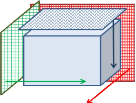
The GPU implementation follows on the same multithreaded structure and adapts it to the GPUs work-items. Given that, in the Young-Van-Vliet´s recursive Gaussian filter, the anti-causal filter takes the output of the causal filter as input, one work-item will apply both filters sequentially on one line of the image in a given dimension. For 2D images, a 1D GPU kernel will be launched; for 3D images, 2D kernels will be used, in order to maximise parallelism.

Figure 2 The figure shows the notion of a 2D kernel (a 2D grid of work-items) that will process the 3D volume in each dimension sequentially.

This is implemented in the GPU kernel method __kernel void partialFilter(

__global const INPIXELTYPE* data, __global OUTPIXELTYPE* outs, __local REALTYPE* Bvalues, __local REALTYPE* MMatrix, unsigned int start,

unsigned int step, unsigned int length )

This method is called in exactly the same way regardless of the dimension (1D, 2D, 3D) of the data to be smoothed.

As an example, in a 3D volume, the line smoothing for dimension Y will be launched as: if(giy < DEPTH && gix < WIDTH) {

partialFilter(data, outs, Bvalues, MMatrix, giy*WIDTH*HEIGHT + gix, WIDTH, HEIGHT); }

In this case, gix and giy identify each work-item uniquely in the 2D grid. Each work-item will know its starting point in the volume of data, depending on this unique id, the length of the vector it needs to process (first with the causal filter, then with the anti-causal) and the step it needs to apply to read the next pixel to process.

B Use of shared and local memory

Another standard strategy to reduce computation time is the use of shared and local memory where possible. To avoid reading from global memory in each calculation, the output of the causal filter is stored in a local memory (i.e. registry-like) array, only accessible by the work-item, and from which the anti-causal filter will read. This way, the input data stored in global memory will only be accessed by the causal pass and the results will then be stored in a local vector.

For reference, preliminary tests indicated that, for a 512x512 double image processed on an nVidia GTX 650, the reduction obtained from not writing the result of the causal pass to global image was of 5.51ms to 4.38ms.

Also, both matrices sent to the GPU are stored in shared memory (visible by all items in a work-group) to avoid reading from global memory for every calculation. Several work-items cooperate to load the values of these matrices simultaneously.

C Fusion of kernels

To avoid unnecessary CPU-GPU synchronisation, it is necessary to apply what Nehab et al. called kernel fusion [7]. On the one hand, as mentioned above, the causal and anti-causal passes (which could have been separated into two independent kernels) have been fused. This is particularly necessary for the Young and Van Vliet IIR filter since the boundary conditions for the transition to the anti-causal filter are initialised using the output values of the causal filter.

On the other hand, each dimension is processed sequentially using as input the output image of the previously filtered dimension, without copying the data on the GPU back to the CPU. It is crucial to avoid a CPU-GPU synchronisation at this point and allow each call of the kernel to access the image stored on GPU memory.

D Work-group sizes

The number of work-items to a work-group is directly related to the number of lines to be processed in a given dimension. It is extremely important to minimise both control divergence and the number of work-items idle.

In the implementation we propose, this is crucial for 3D volumes of different sizes in each dimension. To better understand this, let us imagine a 1024x512x16 sequence. Each dimension will be smoothed separately.

• When filtered in the X dimension the kernel will see the volume as a stack of 1024 images of

size 512x16 images. This means that our 2D work-item grid should be 512x16 and each work-item will process a vector of length 1024.

• When filtered in the Y dimension the kernel will see it as a stack of 512 images of size 1024x16 images. This means that our 2D item grid should be 1024x16 and each work-item will process a vector of length 512.

• Lastly, it follows that in the Z dimension we will need a 1024x512 2D grid of work-items,

each of which will process a data vector of length = 16.

If each kernel call is made with the same grid size (i.e. the same global work-group sizes in both dimensions), and given that only work-items within the boundaries of the volume will have data to process, performance will suffer due to idle work-items and control divergence.

To prevent this, it is necessary to set the global work-group sizes to sizes close to that of the volume. For reference, failing to do this on a 3D volume of 1024x1024x16 caused an increase of time of 38.63ms to 272.43ms.

E Unrolled loops

Loops inside a kernel must be avoided wherever possible. A workaround is to unroll the loops explicitly or using compiler directives such as #pragma unroll [factor]. Certain compilers (e.g. nVidia) unroll loops by default whenever they are controlled by a constant value known at compilation time. However, this is not a requirement in OpenCL specifications (as of 1.1 and 1.2) and failing to unroll the loops either explicitly or via a pragma directive can potentially decrease performance.

6

Results

We present here a subgroup of our results, for different sizes of 2D and 3D images, and sigma = 12. These results were obtained from a machine with the following configuration:

• Intel i7-3770S (8 threads, 4 cores at 3.10GHz),

• 16GB of RAM

• nVidia GeForce GTX650 with 1GB DDR5 RAM (384 cores at 1GHz)

• nVidia drivers 304.84 on Ubuntu.

A Times

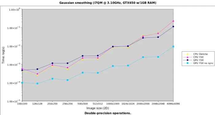
The results show the performance of two CPU implementations (the Young-Van Vliet and the Deriche) and two variations of the GPU Young-Van Vliet implementation (including all data transfers between CPU and GPU and without these data transfer times). The aim of these two GPU times is to show the overhead introduced by data synchronisation.

Figure 3 Results for 2D images, processing with double precision (time in log scale).

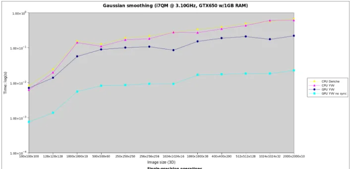
Figure 5 Results for 3D images, processing with double precision (time in log scale).

For 2D images (Figures 3 and 4), the bigger the size, the better the performance factor on GPU. Including GPU-CPU synchronisation overheads, we have obtained a x2 acceleration factor. Without including these overheads (e.g. considering the smoothing as part of a bigger pipeline), the acceleration factor is x24. For 3D images (Figures 5 and 6), the maximum acceleration factor including data transfers was x2.8, whereas without this overhead the acceleration obtained was 31.6.

It is also interesting to see how this GPU implementation of a recursive Gaussian smoothing performs compared to the discrete Gaussian smoothing.

Figure 7 Brief comparison between CPU and GPU implementations of Discrete Gaussian smoothing and Recursive Gaussian smoothing (3D).

Figure 8 Brief comparison between CPU and GPU implementations of Discrete Gaussian smoothing and Recursive Gaussian smoothing (2D).

B Image quality

The difference between CPU and GPU implementations has been measured on the following image (Figure 9). Figures 10 and 11 show the results of smoothing it with sigma = 12 (or variance = 144 in the case of ITK's discrete Gaussian smoothing filter), while Figures 12 and 13 show the root mean square of the difference, pixel by pixel, between the images as smoothed by the CPU and the GPU implementation. The original image, scaled at different sizes, is a JPEG with integer values between 0 and 255.

Sigma=12, var=144 1024x1024x32

CPU Discrete Gaussian 21.629s

GPU Discrete Gaussian 1.969s

CPU Young Van Vliet 0.615s

GPU Young Van Vliet 0.082s

Sigma=12; var=144 1024x1024

CPU Discrete Gaussian 200.205ms

GPU Discrete Gaussian 17.200ms

CPU Young Van Vliet 9.798ms

Figure 9 Original image. Value range: [0, 255].

Figure 10 Smoothed image with [left] CPU and [right] GPU implementations, sigma=12. (Operations in single precision, float.)

Figure 11 Smoothed image with [left] ITK's CPU Deriche recursive Gaussian smoothing filter (sigma=12) and [right] ITK's CPU discrete Gaussian smoothing filter (variance=144). (Single precision.)

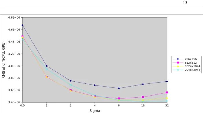
Figure 12 RMS of the difference between the CPU-smoothed image and the GPU-smoothed image, log scale. (Operations in single precision.)

Figure 13 RMS of the difference between the CPU-smoothed image and the GPU-smoothed image, linear scale. (Operations in double precision.)

7

Discussion

This GPU implementation has a strong limitation in the amount of shared memory available, since all intermediate values are stored per work-item on its local memory. Until recently, as shown in studies such as [6], this was a very important reason why recursive algorithms performed poorly on GPUs [7], as opposed to convolution-based algorithms. More recent architectures (e.g. nVidia's Fermi) provide increased shared memory.

An important aspect of GPU programming is the overhead introduced in data synchronisation between CPU and GPU. For each smoothing process, the whole input image -as well as any other data required for the operations- is copied to the GPU and the whole output image is copied back to the CPU. The time required without including data synchronisation is shown under “GPU YVV no sync”. GPU implementations become particularly efficient when several processes can be applied without requiring data to be copied back and manipulated in the CPU (e.g. a pipeline chaining several filters).

This can be observed in the times that include these data transfers. The maximum acceleration that was obtained with the GPU implementation was a x33 factor between the CPU and the GPU implementation of the Young-Van-Vliet algorithm on 3D images, without considering the overheads. The acceleration obtained when including the synchronisation overheads was x3.5.

For 2D images, this improvement was more discrete, with a maximum acceleration of x24 without overheads and x2.2 with the synchronisation overheads.

To put these results in context, it is also interesting to compare them with the Discrete Gaussian (CPU and GPU) implementations already available on ITK (Figures 7 and 8). Both results show that a GPU implementation of the recursive Gaussian filter is a valid alternative to the GPU discrete Gaussian filter in terms of time, even for smaller 2D images. The choice of one over the other depends above all on the power of the CPU and the GPU available, the memory available on the GPU (which, as already mentioned, may hinder recursive algorithms) and the dimensionality of the images.

Thus, it can be argued that with recent GPU architectures, different algorithms need to be benchmarked against the specific needs: 3D images vs. 2D images, CPU and GPU configurations, or the necessary kernel sizes to evaluate the cost of a convolution-based approach.

A possible alternative to this GPU implementation of a recursive Gaussian could be to adapt the Deriche version instead, given that the causal and anti-causal passes can be applied simultaneously (thus giving additional margin for parallelization).

Finally, the differences between CPU and GPU results for floating-point operations must be addressed. Floating-point precision in GPUs has been discussed extensively and Whitehead and Fit-Florea address it regarding Nvidia GPUs specifically (such as the ones used to obtain the results shown here) in [8].

Given how GPUs capable of precision operations are widely available, it is advised to use double-precision operations for the algorithm presented here (option “GPU_HANDLES_DOUBLE” during configuration, as mentioned in Users Guide).

8

Conclusions

An implementation of the Young-Van-Vliet recursive Gaussian filter has been presented for CPU and GPU. It has been discussed that the GPU implementation is a valid alternative to GPU-based discrete Gaussian smoothing and how the choice of one or other algorithm and implementation depends strongly on the hardware configuration (powerful CPU, GPU or both) available to the user.

9

Acknowledgements

Authors would like to thank Jessie Mahé and Nicolas Linard (both from Mauna Kea Technologies, Paris) for their input during this work.

A.

Appendix

Similar tests were carried out on the Gaussian filtering sample CUDA code provided by Nvidia [9]. There are several differences to be remembered while considering these results: namely that the code is meant and optimised to process RGB (not gray-scale) images. However, these results were initially taken as a reference of the speed that could be expected from optimised Gaussian filtering code and are provided here as similar reference and context.

The test image was a 512x512 RGB image. Time measurements include all memory synchronisations between CPU and GPU.

CUDA recursive Gaussian Smoothing: 5.72ms

CUDA separable convolution Gaussian Smoothing, kernel length = 5: 0.49ms

A similarly sized 512x512 gray-scale image is smoothed by the proposed Young & Van Vliet implementation in 2.34ms.

It worth mentioning that the CUDA separable convolution Gaussian smoothing filter is much more efficient than the current implementation of the GPU discrete Gaussian smoothing filter in ITK. The two most likely reasons being the fact that the ITK implementation is not separable and that it is a naive implementation, that is, it does not apply certain GPU coding techniques discussed above (namely, the use of shared memory instead of global memory and tiling) are not applied.

Reference

[1] R. Deriche. Recursively implementing the Gaussian and its derivatives. Int. Conf. Image Processing, Singapore, 1992.

[2] I. Young and L. van Vliet. Recursive implementation of the Gaussian filter. Signal Processing, vol. 44, pp. 139–151. 1995.

[3] I. Young, L. van Vliet, and M. van Ginkel. Recursive Gabor filtering. IEEE Transactions on Signal Processing, vol. 50, no. 11, pp. 2799–2805. 2002.

[4] B. Triggs and M. Sdika. Boundary Conditions for Youg – van Vliet Recursive Filtering. IEEE Transactions on Signal Processing, vol. 54, no. 5. 2006.

[5] J. M. Geusebroek, A. W. M. Smeulders, and J. van de Weijer. Fast anisotropic gauss filtering. IEEE Trans. Image Processing, no. 12, pp. 938-943. 2003.

[6] X. Wang and B. Shi. GPU implemention of fast gabor filters. Proc. ISCAS, no. 30. 2010.

[7] D. Nehab, A. Maximo, R. S. Lima, H. Hoppe. GPU-Efficient Recursive Filtering and Summed-Area Tables. ACM Trans. Graphics (SIGGRAPH Asia). 2011.

[8] N. Whitehead, A. Fit-Florea. Precision & performance: Floating point and IEEE 754 compliance for NVIDIA GPUs. NVIDIA Technical White Paper. 2011.