OATAO is an open access repository that collects the work of Toulouse
researchers and makes it freely available over the web where possible
Any correspondence concerning this service should be sent
to the repository administrator:
[email protected]
This is an author’s version published in:
https://oatao.univ-toulouse.fr/27148
To cite this version:
Lazhar, Ramzi and Najjari, Mustapha and Prat, Marc Combined
wicking and evaporation of NaCl solution with efflorescence
formation: The efflorescence exclusion zone. (2020) Physics of
Fluids, 32 (6). 067106. ISSN 1070-6631
Open Archive Toulouse Archive Ouverte
Official URL :
Combined wicking and evaporation of NaCl
solution with efflorescence formation:
The efflorescence exclusion zone
Ramzi Lazhar,1 Mustapha Najjari,1 and Marc Prat2,a)
AFFILIATIONS
1Université de Gabès, Ecole Nationale d’Ingénieurs de Gabes, LR18ES34, 6072 Zirig, Gabes, Tunisia
2Institut de Mécanique des Fluides de Toulouse (IMFT), Université de Toulouse, CNRS –31400, Toulouse, France a)Author to whom correspondence should be addressed:[email protected]
ABSTRACT
An experiment combining wicking and evaporation of a NaCl solution and leading to the formation of salt efflorescence is presented. The experiment shows that efflorescence develops over the porous medium surface exposed to evaporation except in the bottom region of the sample. This region remains free of efflorescence and is called the exclusion zone. It is shown that the exclusion zone extent depends on the solute concentration in the bottom reservoir. A model is developed, and it helps understand the exclusion phenomenon. The arch shape of the exclusion zone upper boundary is explained and modeled. The study is also seen as a successful test for the model of efflorescence growth driven by evaporation and salt precipitation presented in a previous study. The modeling approach is expected to help develop better models of salt transport with crystallization at the surface of porous media in relation with soil salinization issues or the salt weathering of porous materials.
https://doi.org/10.1063/5.0007548
I. INTRODUCTION
Crystallization of salt in porous media is one of the major causes of the damage both in cultural heritage and in civil engineer-ing constructions. Also, salt crystallization at the surface of a soil can severely affect evaporation and, thus, soil–atmosphere exchange. These applications have motivated quite a few works, e.g., Refs.1–7, to name only a few. Modeling this type of situation implies deal-ing with the trio: evaporation, ion transport in solution within a porous medium, and crystallization. Despite the significance of the aforementioned applications and the numerous publications, devel-oping predictive models and validating them against experimental data are still largely an open question, at least when a significant crystallization takes place. In this respect, it is convenient to distin-guish two main situations as discussed, for instance, in Ref.8: drying and evaporation-wicking. Consider an initially wet porous sample. Drying9,10is typically when there is no supply in solution during evaporation. In contrast, evaporation–wicking11is when the solu-tion can be sucked, typically by the capillary effect, into the sample
so as to compensate, at least partly, the evaporation. As discussed in Ref.11, the sample can actually stay fully saturated when the solution absorption rate fully compensates the evaporation. In what follows, we are interested in this situation. Hence, the material will be sat-urated all the time. In practice, this situation can be encountered where a construction is in contact with natural groundwater or in a marine environment. A well-known example is the constructions in the city of Venice. The situation before the onset of crystallization is less tricky, and reasonably reliable models can be used to predict the ion distribution within a porous sample exposed to evaporation. In the case of the evaporation–wicking situation, one can refer, for instance, to Ref.11, where it is shown that using the standard macro-scopic convection–diffusion equation for the ion transport leads to fairly good results. The solution developed in Ref.11corresponds to a quasi-1D situation where evaporation occurs only at the top surface of the sample, the solution is supplied through the sample bottom surface, and the sample lateral sides are impervious. We con-sider the somewhat different situation where evaporation takes place not only at the top surface but also along the lateral sides. This is
FIG. 1. SEM-EDS analysis of the surface ceramic. Top: SEM image perpendicular
to the sample surface, pores correspond to black spots in the image; bottom: EDS spectrum of the ceramic.
also a classical situation, notably considered in laboratory tests.12,13 More importantly, we are interested in the situation where a quite significant development of salt (NaCl) crystals takes place. The study combines experiment and modeling. In the experiment, salt efflores-cence develops covering a quite significant fraction of the evapora-tion surface of the porous medium. Interestingly, however, a notice-able fraction of the evaporation surface stays free of efflorescence. This phenomenon is referred to as the exclusion effect. The experi-ment indicates that the spatial extension of the exclusion zone varies with the solute concentration in the solution reservoir into which
the sample bottom region is plunged. In the present state of the art in the concerned research area, the exclusion zone phenomenon can be seen as an interesting modeling challenge since it is observed in a situation where crystallization is quite significant. In other words, can we understand the exclusion effect and propose a predictive model? In addition to highlighting and describing the efflorescence exclusion effect, answering these questions is the main objective of the present paper. It is organized as follows: The porous material and the experimental setup are described in Secs.IIandIII, respectively. Experimental results are presented in Sec.IV. Modeling is presented in Sec.Vtogether with comparisons with the experimental results. A short discussion is proposed in Sec.VI. Conclusions are drawn in Sec.VII.
II. POROUS MATERIAL
The porous medium is a glazed ceramic (Faience tile—Tunisian industry). This material has been used in buildings for decoration of inner and outer walls of private houses, historic monuments, and state buildings. Particle-induced x-ray diffraction (XRD), electron microprobe analysis [energy dispersive spectra (EDS)], and scanning electron microscopy (SEM) analytical techniques were used to char-acterize the surface of the material. Major, minor, and trace elements were detected by XRD, and SEM-EDS gave information on the main mineral phases. The main mineral of the porous ceramic sur-face, identified by x-ray diffraction, is the quartz (SiO2). The main major chemical elements obtained by SEM-EDS are SiO2, CaCO3, MgO, Al2O3, GaP, FeS2, and TiO2. Therefore, the conclusion is that there is no internal source of NaCl in this material.Figure 1
displays the characteristics of the surface by SEM images and EDS semi-quantitative analyses.Table Ishows the chemical composition corresponding to the spectrum shown inFig. 1.
The porosity accessible to water, denoted by εpm, was deter-mined on pieces of ceramic according to the American Technique Standard (ASTM C642-97).14This gave εpm ≈ 0.2. As indicated in
Fig. 1, relatively big pores, on the order of a few tens of micrometers, are present.
III. EXPERIMENTAL SETUP
Five pieces, referred to as A1, A2, A3, A4, and A5, were cut in rectangular shape from a glazed ceramic, keeping the glazed side as one side of the sample. Dimensions of these samples are given in
Table II. Initially, all samples were dried. Sample A1 was saturated with pure water. The other samples were contaminated by NaCl by immersion in an aqueous solution. Various salt concentrations were considered as indicated inTable II. When all samples were fully saturated, they were set vertically in reservoirs filled with the
TABLE I. Mean percentage of chemical composition of the studied ceramic surface expressed as wt. % and at. % obtained by means of SEM-EDX analysis.
Element Si O Ca Mg C P S Ti Fe Mn Al K
wt. % 27.85 45.11 2.29 1.55 4.27 0.32 0.16 0.50 6.32 0.09 8.06 2.75
TABLE II. Sample geometrical dimensions and initial NaCl concentration for the various samples [seeFig. 2(b)for the notations, Ht= H + Hi]. The exclusion length Heis the height of the region free of efflorescence at the end of the experiment. As shown inFig. 6, it is measured in the middle of the front face as the vertical distance between the bottom of the non-immersed part of the sample and the first crystals at the surface. The solubility ion mass fraction is 0.264 (which corresponds to 6.1M).
Immersion solution
(NaCl mass H(cm) Hi(cm) Ht(cm) He(cm)
Sample fractionC0) (external length) (immersed length) (total length) w (cm)(width) e (cm) (thickness) (exclusion length)
A1 Pure water 11 5.5 16.5 7.5 0.6 . . .
A2 0.1 11 5.5 16.5 7.5 0.6 6.5
A3 0.15 11 5.5 16.5 7.5 0.6 5
A4 0.2 11 5.5 16.5 7.5 0.6 3.5
A5 0.25 11 5.5 16.5 7.5 0.6 2
corresponding saturating solution (Fig. 2), i.e., with the composi-tion same as that of the one used to soak the sample. The immersion depth of a sample in the reservoir was 5.5 cm. The presence of the reservoir ensured a continuous supply of the solution to the sample and then compensates the loss of water resulting from evaporation.
As shown inFig. 2, the upper part of the samples was exposed to evaporation. Note that no relative humidity and temperature control were imposed in the experiment room.Figure 3shows the relative humidity and temperature variations measured in the experiment room during the experiment. Also, note that the back face of the samples corresponds to the glazed surface. As a result, there was no evaporation from the back face. As sketched inFig. 2(b), evapora-tion occurred at the top surface, the front face, and the two lateral faces.
As illustrated inFig. 2, the reservoirs were well closed except for the opening hole on the top surface used to introduce the sample. Thus, one can consider that the direct evaporation of the solution from the reservoir, if any, was quite limited. The mass loss of each system (sample and reservoir) due to evaporation was measured by using an electronic balance with an accuracy of±0.001 g. The devel-opment of the efflorescence and its distribution on the evaporation
FIG. 2. (a) Porous sample partially immersed in the bottom reservoir at the
beginning of the experiment and (b) sketch of the studied system with the main notations.
surface of the samples were recorded during 10 days using a camera with a resolution of 4160× 2336 pixels2.
IV. EXPERIMENTAL RESULTS
A. Salt crystallization dynamics: The efflorescence exclusion zone
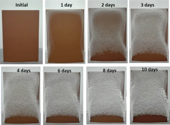
Figure 4shows images of the efflorescence development over the surface at different times for the initial ion mass fraction C0 = 0.25. The images actually correspond to a preliminary experiment. The relative humidity and temperature were not recorded in this preliminary experiment, and only two NaCl initial concentrations were considered. For this reason, the experiment was repeated with more NaCl initial concentrations and with the relative humidity and temperature measurements. For the same initial salt mass fraction,
FIG. 3. Relative humidity Hr,infand temperature variations in the experiment room
FIG. 4. Typical efflorescence development over the sample surface for C0= 0.25.
both experiments led to the same exclusion zone, which is seen as a good repeatability test. Efflorescence is visible after about one day along the edges of the sample front face. The evaporation flux is expected to be higher at the edges, and it is known that crystallization first occurs where evaporation is greater.18,19Actually, as discussed in Sec.V B, the edge effect, i.e., the fact that crystallization begins in the edge regions, can be present even with a uniform evaporation flux due to the combined impact of the evaporation from the front face and from the lateral faces in the edge region. Then, the efflores-cence spreads on the evaporation surface, from top to bottom and from the ridges of the sample to the surface middle.
In this example, the surface colonization process takes about one day (compare the image after one day and after two days in
Fig. 4). One can wonder whether this surface colonization process has to do with salt creeping,20i.e., seen here as the lateral develop-ment of the efflorescence from the previous efflorescence salt crystals or simply results from crystallization in new pores at the ceramic surface, as in Ref.19, for instance, or a mix of both processes. This cannot be deciphered from the data of the present experiment. In any case, it can be seen that the extent of the zone occupied by the efflorescence stabilizes. One can note some additional colonization at the bottom of this zone during the next day (day 3) and that the efflorescence zone gets whiter and whiter, which is a clear indication that the precipitation process continues during the experiment and takes place on top of the efflorescence already in place.
However, the most remarkable and somewhat unexpected fact is that no crystallization of salt is observed during all the experiments in the bottom region of the sample inFig. 4. This region is referred to as the efflorescence exclusion zone, and the corresponding phe-nomenon is referred to as the exclusion phephe-nomenon. Since this part of the sample is the closest to the sample immerged part, i.e., to the solute source, one could think that this zone should see the forma-tion of efflorescence. This is clearly not the case. It can be seen that the extent of this zone is quite stable (comparing the image for day ten with the image for day four inFig. 4). Another interesting fea-ture is the arch shape of its upper boundary, which is interpreted as a consequence of the locally higher evaporation at the edges, due to the contribution of the lateral faces and possibly of a higher external demand in the edge region, compared to the region of the surface away from the edges.
Additional insights on the exclusion zone can be obtained from the images shown inFig. 5. In particular, it can be seen that the size of the exclusion zone increases when the reservoir ion mass fraction is decreased.
In summary, a quasi-steady state is reached, in which the efflo-rescence develops over only a fraction of the sample surface exposed to evaporation. The remaining fraction at the bottom is free of efflo-rescence. The initial NaCl concentration has an impact on the exclu-sion zone extenexclu-sion. The greater the initial concentration, the lower the extent of the exclusion zone, all other factors being equal.
FIG. 5. Top: development of efflorescence over the sample surface at the end of the experiment for the various samples. Impact of the solution concentration in the bottom
reservoir. The height of the exclusion zone decreases as the NaCl mass fraction in the reservoir increases. Bottom: efflorescence (in red) and exclusion zone (blue with possible color variations between blue and lighter red) computed using the 2D model described in Sec.V B.
The objective is now to understand and explain these trends from simple modeling considerations. However, some considera-tions on the evaporation results are necessary beforehand.
B. Evaporation kinetics
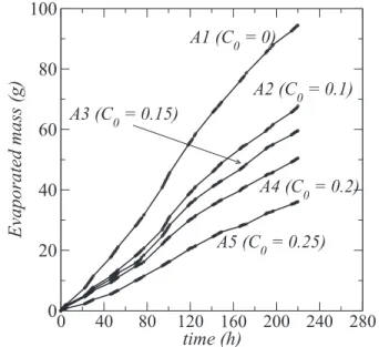
The measured cumulative mass lossme(t) as a function of time for the various samples is shown inFig. 6.me(t) is computed as
me(t) = m0− m(t), (1)
wherem(t) is the mass of the system (sample + reservoir) and m0is the mass att = 0; me(t) corresponds to the mass of water leaving the system by evaporation.
The evaporation rate can be computed from these data as follows:
J=dme
dt . (2)
Then, one can determine the mean evaporation fluxj for each porous sample as j=J S= 1 S dme dt , (3)
whereS is the total sample surface area open to evaporation. Thus, with the notations indicated inFig. 2(b),S = ew + wH + 2eH (it is recalled that there is no evaporation from the sample back face).
As can be seen fromFig. 6, the evaporation rate (the slope of the curves in Fig. 6) does not change very significantly over the duration of the experiment. Since, as discussed before, the forma-tion of efflorescence is quite significant and takes place early in the
experiment, this is a clear indication that the efflorescence develop-ment does not affect very much the evaporation rate. As reported in Refs. 15,16, one can distinguish two main types of efflores-cence: blocking and non-blocking. Blocking efflorescence refers to the efflorescence that severely reduces the evaporation rate com-pared to the evaporation rate before the efflorescence development. It corresponds to the “crusty” efflorescence in Ref.15. The plot of the evaporated mass as a function of time is characterized in this case by a marked change in the slope of the evaporated mass curve, which tends to become flat. In contrast, the non-blocking efflores-cence does not affect very much the evaporation rate, i.e., the slope of the curveme(t) does not vary very much. Thus, referring to this clas-sification, the efflorescence is our experiments can be considered as non-blocking. This corresponds to a porous efflorescence in which the solution is sucked by capillarity up to the efflorescence external surface where water evaporates and salt precipitation makes grow the efflorescence, e.g., Refs.17, and 18. The slight changes in the slope of the curves inFig. 6can be explained by the variation of the relative humidity in the experiment room. As can be seen from
Fig. 3, the relative humidity drops after about 80 h. This well corre-sponds to the increase in the slopes of the curves inFig. 6, i.e., to an increase in the evaporation rate.
The evaporation rate is typically proportional to the difference between the water vapor partial pressure at the porous sample sur-facepvsand the water vapor partial pressurepvinf .in the room away from the sample:
J∝ (pvs− pvinf .) . (4)
In the case of pure water,pvs=pvsat, wherepvsatis the saturated water vapor pressure. In the case of the NaCl solution, the solution at the surface is expected to be salt saturated, i.e., at the solubility, at least over the fraction of the surface covered by the efflorescence. The presence of the ions in the solution reduces the water activity. For a saturated NaCl aqueous solution,pvs= 0.75pvsat. Thus, it is expected that the ratio of the evaporation rate between the pure water sat-urated sample and the sample A5 for which the ion mass fraction everywhere at the surface can be expected to be close to solubility
(since the ion mass fraction in the reservoir is close to solubility for sample A5) verifies
JA1 JA5≈ (pvsat− pvinf .) (0.75pvsat− pvinf .)= (1 − Hr,inf) (0.75 − Hr,inf) , (5)
whereHr ,infis the relative humidity in the experiment room. With, for instance,Hr ,inf = 0.52, which is the average value over the last 24 h period of the experiment (seeFig. 3), one obtains JA1
JA5 ≈ 2
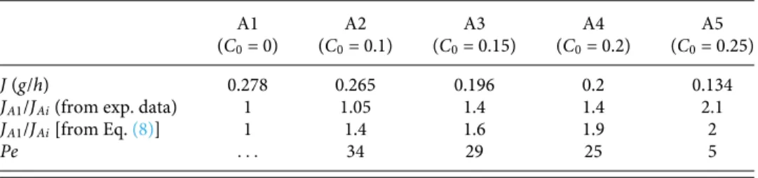
(as reported in Ref. 15, this ratio is at least one order of magni-tude greater when the efflorescence is blocking).Table IIIshows this ratio computed from the slopes of theme(t) curves over the last 24 h period of the experiment, i.e., betweent = 196 h and t = 220 h. As expected, JA1
JA5 ≈ 2 for sample A5. This ratio is less than 2 for the
other samples, i.e., the evaporation rate is closer to the one for pure water. This is consistent with the fact that the ion mass fraction is actually lower than the solubility over a fraction of the sample sur-face, i.e., the fraction of the surface not covered by the efflorescence. The latter consideration can be further supported by the following estimates. The computation of the ion mass fraction field presented later in the paper indicates that the ion mass fraction field is close to the reservoir ion mass fractionC0over most of the surface free of efflorescence. Thus, a more refined estimate of the evaporation rate can be obtained by adding the contribution from the region cov-ered by the efflorescence to the contribution from the region free of efflorescence, JAi= JAi-free-surface+JAi-efflorescence, (6) which leads to JAi∝ (w + 2e)HeMv RT(pvs(C0) − pvinf .) +((w + 2e)(H − He) + we)Mv RT(pvs(Csat) − pvinf .), (7) where Mv is the vapor molecular weight, R is the universal gas constant, andT is the temperature. This leads to
JA1 JAi ≈
((w + 2e)H + we)(pvsat− pvinf .)
(w + 2e)He(pvs(C0) − pvinf .) + ((w + 2e)(H − He) + we)(pvs(Csat) − pvinf .)
, (8)
TABLE III. Evaporation rate at the end of experiment for each sample, the evaporation rate ratio (evaporation rate for pure water/evaporation rate for the saline solution), and the Peclet number for the various samples.Pe = Vz(0)He
εpmD∗
s , where Heis
the exclusion height as computed from Eq.(16), Vz(0) is the filtration velocity at the sample inlet,εpmis the porous medium porosity, andD∗
s is the solute effective diffusion coefficient in the porous medium.
A1 A2 A3 A4 A5
(C0= 0) (C0= 0.1) (C0= 0.15) (C0= 0.2) (C0= 0.25)
J (g/h) 0.278 0.265 0.196 0.2 0.134
JA1/JAi(from exp. data) 1 1.05 1.4 1.4 2.1
JA1/JAi[from Eq.(8)] 1 1.4 1.6 1.9 2
which gives the values reported inTable III(to determine the equi-librium vapor pressure for the different values of the ion mass frac-tionC0, we have used the data presented in Ref.21). The trend in
Table III, i.e., the fact that the evaporation rate ratio decreases as the reservoir ion mass fraction is decreased, is consistent with the fact that the free surface fraction increases as the reservoir ion mass fraction is decreased.
Considering the assumptions and simplifications made, i.e., notably, the fact we have implicitly assumed an uniform external mass transfer coefficient all over the surface, our conclusion is that the comparison between the results from Eq.(8)and the estimates from the experimental data inTable IIIis sufficiently good for sup-porting the following main consideration: evaporation takes place all over the surface, i.e., where there is no efflorescence, as well as where the efflorescence is present.
The conclusion is, therefore, that the efflorescence is not block-ing in our experiment and that the lower evaporation rate observed with the saline solution is simply due to the lower activity of the solution compared to pure water. Also, the picture is that, in the quasi-steady regime reached by the system, evaporation takes place all over the surface, i.e., the surface fraction free of efflorescence, as well as the surface fraction covered by the efflorescence.
V. MODELING
A. Extent of the exclusion zone
Based on the elements discussed in Sec.IV, it is assumed that a quasi-steady regime is reached. Also, the evaporation is little affected by the efflorescence development. Thus, the solution is continuously absorbed by the sample. The ions are transported within the sample up to the surface of the efflorescence where precipitation occurs. If we denote the solute mass flow rate at the sample inlet by ϕinl.and the precipitation rate at the efflorescence surface by ϕeffl., then it is expected that ϕinl.≈ ϕeffl.. The latter equality simply means that all the ions entering the sample eventually lead to the formation of new crystals at the external surface of efflorescence. It cannot be excluded that new crystals also form within the efflorescence and/or possi-bly within the porous sample region adjacent to the efflorescence. However, this is neglected, and we only consider precipitation at the efflorescence external surface. The next step is to express ϕinl.and
ϕeffl.. Throughout the analysis, we assume that the evaporation flux is the same everywhere at the sample evaporation surface and, thus, equal to the mean evaporation flux given by Eq.(3). This is a simpli-fication since it is likely that the evaporation flux varies spatially. To express ϕeffl., we use the expression of the efflorescence local growth rate φ derived in Ref.22, namely,
φ=Csat(ρCsatε + ρcr(1 − ε)) ρcr(1 − ε)(1 − Csat) [
Da
1 +Da]j, (9)
where ρ is the density of the solution, ρcris the crystal density, ε is the efflorescence porosity,Da is a Damkhöler number characterizing the competition between the precipitation reaction and the diffusive ion transport in the efflorescence, andCsatis the equilibrium ion mass fraction in a saturated solution (Csat= 0.264). In fact, the ion mass fraction on top of the growing efflorescence is greater thanCsatsince supersaturation is necessary for the precipitation to occur. However, as discussed in Ref.10and also shown in Ref.22, the supersaturation
is actually very close to the saturation concentration when new crys-tals form in the presence of already existing cryscrys-tals. As a result, the approximationC≈ Csatis made in deriving Eq.(9). One can refer to Refs.10and22for more details. With the notations inFig. 2(b), this leads to express ϕeffl.as
ϕeffl.= ((H − He)(w + 2e) + we)φ, (10) and, thus, to
ϕeffl.= ((H − He)(w + 2e) + we)λj, (11) where
λ=Csat(ρCsatε + ρcr(1 − ε)) ρcr(1 − ε)(1 − Csat) [
Da
1 +Da] . (12)
To express the incoming solute mass flow rate, we first note that the velocity induced in the solution as a result of the local evapora-tion and local efflorescence growth can be expressed according to Ref.22as ρV= (1 + α)j, (13) where α=Csat(ρε + ρcr(1 − ε)) ρcr(1 − ε)(1 − Csat)[ Da 1 +Da] . (14)
Equation(13)applies over the sample external surface where the efflorescence is present. In the exclusion zone, the velocity nor-mal to the surface is simply V = ρj. This leads to express ϕinl. as
ϕinl.= C0[((H − He)(w + 2e) + we)(1 + α)
+He(w + 2e)]j − weρεpmD∗sB1, (15) whereC0is the ion mass fraction in the reservoir, εpmis the porous sample porosity, andD∗
s is the effective diffusion coefficient of the ions in the porous sample. The factorB1comes from the steady-state solution of the convection–diffusion problem in the efflorescence free region located betweenz = 0 and z = He. Its expression is derived in theAppendix. It notably depends onHe.
After some algebra, expressing that ϕeffl.= ϕinl.yields He− we (w + 2e) ρεpmD∗sB1 j(λ − C0α)= H(1 − C0 (λ − C0α)) + we (w + 2e)(λ − C 0(1 + α)) (λ − C0α) , (16)
which is used in what follows to determine the exclusion zone height Heas a function of the bottom reservoir solute mass fractionC0. To this end, we have to specify the Damkhöler numberDa and the efflo-rescence porosity ε in order to determine λ and α from Eqs.(12)and
(14). Although the determination of efflorescence porosity is still an open question, we have taken ε = 0.1 since the porosity is a priori expected to be not too high. RegardingDa, we have tried the value of 4 used in Ref.22.
As depicted inFig. 7, a good trend is obtained, but the exclu-sion length is significantly underestimated for the greater reservoir ion mass fractions. According to Ref.22,Da can be computed as
FIG. 7. Computed exclusion height as a function of the reservoir ion mass fraction.
The red square symbols correspond to the experimental exclusion height deter-mined as indicated inTable IIIand illustrated inFig. 5. The blue circles correspond to the results of the 2D simulations (see Sec.V B) and the dashed lines to Eq.(16)
for two values of the Damkhöler number Da.
Da = √
(1−ε)2(1−C sat)kr
εD∗
sav , whereavis the pore wall surface area per
unit volume andkris the precipitation coefficient (kr ≈ 2.3 × 10⁻³ m/s23). As in Ref.22, we assumed thatav could be estimated as av = 3(1−ε)r
b , whererbis an equivalent grain size. Since the
efflo-rescence is not blocking in the experiment and looks a bit like small cauliflowers in some areas, it can be expected that the pores in the efflorescence are bigger than in the salt crust considered in Ref.22
(rb∼ 0.6 μm). With rb∼ 10 μm for instance, one obtains Da ≈ 10, thus greater than in Ref.22. We have interpreted this result as an indica-tion thatDa was probably greater in the case of our experiments than for the compact crust considered in Ref.22. For sufficiently high Da, i.e., above about 50, λ and α become essentially independent of Da (since the ratio Da
1+Da ≈ 1). If we assume that Da for our efflo-rescence is sufficiently large for Da
1+Da ≈ 1, we obtain from Eq.(16) the results depicted in Fig. 7(Da = 100). As can be seen, greater exclusion lengths are obtained in the range of the greater values of C0, and a quasi-linear variation ofHewithC0is obtained as in the experiments.
However, the slope is different and greater than in the experi-ment. Nevertheless, since Eq.(16)is based on a simple mass balance and a slice average 1D solution, it can be reasonably concluded that the proposed approach captures the essential ingredients at play. In
Fig. 7, we have indicated the predictions of the 2D model presented in Sec.V B(for the case where1+DaDa ≈ 1). This model can be seen as a 2D version of the simpler 1D model leading to Eq.(16). However, the 2D model cannot be solved analytically. As can be seen from
FIG. 8. Typical average ion mass fraction profile along the sample height computed
from Eq.(A11)in theAppendixfor C0= 0.15.
Fig. 7, the consideration of the 2D model improves the comparison with the experiments.
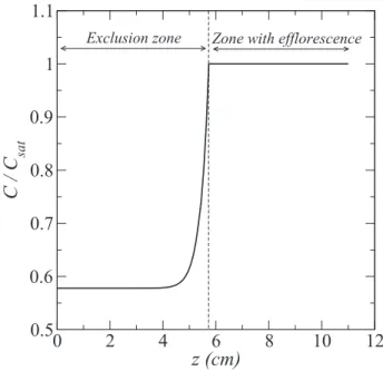
Additional insights can be gained from the slice averaged ion mass profile depicted inFig. 8for the condition of experiment A3 (C0= 0.15).
This profile was computed from Eq.(A11)in theAppendix. In the region where the efflorescence is present at the surface, i.e., forHe ≤ z ≤ H, C ≈ Csat. This is actually an assumption supported by the fact that the ion mass fraction in the efflorescence is the solubility mass fraction.22In the zone free of efflorescence, i.e., 0≤ z ≤ He, a typi-cal exponential-like profile is obtained (as shown in theAppendix, it is not exactly exponential because the velocity decreases along z). Based on previous studies, i.e., Ref.11and references therein, this type of profile is expected when the ion advection is noticeable com-pared to diffusion. Although the vertical velocity varies alongz in our case, this can be evaluated from the Peclet numberPe=Vz(0)He
εpmD∗ s .
For experiment A3, one obtainsPe≈ 29, thus greater than 1, which is consistent with the profile depicted inFig. 8. Estimated values of Pe for all the samples are indicated inTable III.
This profile illustrates the fact that the ion mass fraction is lower than the solubility throughout the exclusion layer, consistent with the fact that no crystallization occurs in this zone.
B. On the arch shape of the exclusion zone: Efflorescence boundary
As illustrated inFig. 6, another intriguing feature of the exclu-sion zone is the arch shape of its upper boundary. It can be surmised that this has to do with either a greater evaporation flux on the edge or with the impact of the evaporation from the lateral faces or both. In any case, evaporation is greater in the region near the edge com-pared to the region of the front face away from the edges. In this
section, a 2D model is developed for computing this shape. Since the analysis presented in SubsectionV Asuggests that the system reaches a quasi-steady regime, steady-state equations are considered in what follows. The flow within the porous sample is modeled using Darcy’s law considering only the viscous effects and the mass balance equation as follows:
∇ ⋅ (ρV) = 0, (17)
V= −K
μ∇P, (18)
whereK is the porous sample permeability and μ is the solution dynamic viscosity.
The boundary conditions at the evaporative surface read
V⋅ n = j
ρ, (19)
where no efflorescence is present (exclusion zone) and
V⋅ n = (1 + α)j
ρ , (20)
where the efflorescence is present. At the top surface of the immersed region (which corresponds to the bottom surface of the computa-tional domain), the pressure is specified:
P= Pbot.at z= 0 . (21)
The solute transport governing equation reads ∇ ⋅ (ρVC) = ∇ ⋅ (ρεD∗
s∇C) − (1 − C)avρkr(C − Csat), (22) while the associated boundary conditions at the evaporative surface read
(ρVC − ∇ ⋅ (ρεD∗
s∇C)) ⋅ n = 0, (23)
where the efflorescence is not present and (ρVC − ∇ ⋅ (ρεD∗
s∇C)) ⋅ n = λj, (24)
where the efflorescence is present.22 At the bottom surface of the computational domain, the bottom reservoir solute concentration is imposed, namely,
C= C0atz= 0 . (25)
In order to obtain a 2D model, the abovementioned equations are averaged over the thicknesse of the porous sample using the operator⟨⋅⟩ =1 e∫ e 0dy. This leads to ∂ ∂x(ρVx) + ∂ ∂z(ρVz) − ρVy]y=0= 0, (26) ∂ ∂x(ρVx) + ∂ ∂z(ρVz) = Ψ , (27)
or after combination with Darcy’s law, ∂ ∂x(ρ K μ ∂P ∂x) + ∂ ∂z(ρ K μ ∂P ∂z) = −Ψ , (28) where Ψ= −(1 + α)j e, (29)
where the efflorescence is present and
Ψ= −j
e, (30)
where there is no efflorescence. Boundary conditions(19)–(21)still apply on the boundary of the 2D computational domain now con-sidered. The governing equation for the solute transport takes the following form: ∂ ∂x(ρVxC) + ∂ ∂z(ρVzC) = ∂ ∂x(ρεD ∗ s ∂C ∂x) + ∂ ∂z(ρεD ∗ s ∂C ∂z) + Ψs − ξ(C − Csat)(1 − C)avρkr(C − Csat), (31) where
Ψs= −
λj
e, (32)
where the efflorescence is present and
Ψs= 0, (33)
where there is no efflorescence.
ξ(C− Csat) is the Heaviside function. Thus, the source term−(1 − C)avρkr(C− Csat) in Eq.(31)is present only whereC≥ Csat.
Boundary conditions (19)–(21) still apply but only on the lateral boundaries of the 2D computational domain.
Naturally, the main unknown is the position of the efflores-cence boundary, which corresponds to the lowerCsatisoline in the computational domain. In order to determine this position, an iter-ative method is used. A first computation is performed assuming no efflorescence. This leads to an ion mass fraction field where the ion mass fraction is much aboveCsatin many places. Then, the bound-ary conditions are modified depending on whetherC≥ Csatat the considered location. This process is repeated until stabilization of the region where C≈ Csat. The solution was obtained using the commercial simulation software COMSOL Multiphysics.
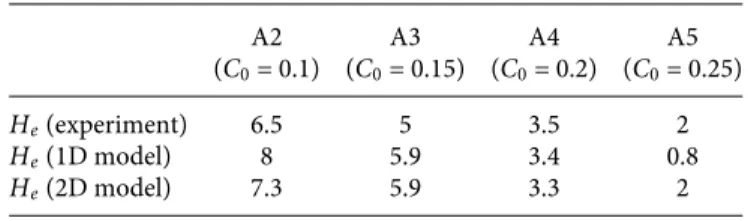
The solution typically gives the 2D distribution of the thick-ness averaged ion mass fractionC over the computational domain. With this model, the efflorescence zone corresponds to the region where C ≈ Csat, whereas the exclusion zone corresponds to the region whereC < Csat. The obtained ion mass fraction fields so obtained are shown inFig. 6together with the experimental efflo-rescence distributions. As can be seen, the model captures quite well the arch shape of the exclusion zone upper boundary. The impact of the bottom reservoir ion mass fractionC0on the spa-tial extension of the exclusion zone is well reproduced. As shown inFig. 7and reported inTable IV, the exclusion heightHeis quite well predicted for A4 and A5 but overestimated for A2 and A3.
TABLE IV. Efflorescence exclusion height He(cm). Comparison between the experi-mental measurement and the predictions of the 1D and 2D models in the limit of large
Da for the four samples.
A2 A3 A4 A5
(C0= 0.1) (C0= 0.15) (C0= 0.2) (C0= 0.25)
He(experiment) 6.5 5 3.5 2
He(1D model) 8 5.9 3.4 0.8
He(2D model) 7.3 5.9 3.3 2
Overall, the 2D model leads to a clear improvement compared to the simpler 1D model. Based on the impact of the Damkhöler num-ber on the 1D results (Fig. 7), the comparison between the 2D model and the experimental results could be probably improved by play-ing withDa (here, we have only considered the case where Da is sufficiently large for 1+DaDa ≈ 1). However, we consider the results shown inFigs. 6and7as sufficiently convincing within the frame-work of the assumptions and simplifications associated with the model.
VI. DISCUSSION
To the best of our knowledge, there is no previous work pre-senting a model similar to the one presented in Sec. V Bwhere the impact of the efflorescence development is taken into account through specific boundary conditions. Naturally, models taking into account the salt precipitation effect have been developed, e.g., Refs.1
and2, but the precipitation in this model typically occurs within the pores of the porous substrate. This corresponds to subflorescence formation and not to efflorescence formation. This is an important difference because the efflorescence typically grows at the surface of the porous medium and not within the pores of the porous substrate. Actually, some precipitation can also occur in the pores close to the surface. This phenomenon has not been taken into account in our model considering that the major mechanism was the efflorescence external growth.
The comparison between the two versions of the model (1D and 2D) and the experimental results is not perfect. The exclusion zone upper boundary arch shape is well reproduced by the 2D model, and the impact of the bottom reservoir ion mass fraction is well cap-tured. However, the prediction of the exclusion zone extent is not very accurate. This could be explained by some assumptions made in the modeling. For instance, we have totally ignored the proba-ble spatial variations of the evaporation flux over the sample surface. The inspection of the efflorescence inFig. 6suggests a greater evap-oration flux in the bottom of the efflorescence region zone since the efflorescence is more developed in this region. Also, we have neglected the possible variations of the efflorescence properties over the surface, its porosity, for instance.
We know from previous studies, e.g., Ref.15, that the efflores-cence can also severely reduce the evaporation rate due to pore clog-ging within the efflorescence. This notably depends on the porous substrate pore sizes and the evaporative demand. Therefore, the sit-uation could be different when the conditions are such that the
efflorescence formation reduces the evaporation rate significantly. In other words, our model does not take into account the possi-ble salt precipitation within the efflorescence pores that can lead to efflorescence pore clogging. This was neglected on the ground that there is no noticeable effect of the efflorescence development on the evaporation rate in the experiment. A more refined approach would be to include this effect in the modeling so as to be able to deal also with situations where the efflorescence formation significantly reduces the evaporation.
The analysis and models make use of the efflorescence growth rate expression derived in a recent article.22 In this respect, the present study can be seen as a reasonably successful test for this expression and, thus, the modeling of the efflorescence growth. However, this model was used considering a Damkhöler number value significantly greater than in Ref.22. Consistent with previous studies, i.e., Ref.15, this indicates that different efflorescence growth regimes exist depending on the conditions (evaporative demand, porous medium pore sizes, etc.). It is surmised that the regime observed in our experiment belongs to the same category as the “patchy” regime described in Ref. 15where the efflorescence for-mation had a very little impact on the evaporation. This type of regime could correspond to relatively high Damkhöler numbers, whereas lower Damkhöler could characterize the regimes where the efflorescence formation does have a detrimental impact on the evap-oration. In this respect, it would be interesting to study whether the exclusion zone still persists when the efflorescence severely reduces the evaporation. However, these considerations are mere specula-tions at this stage. Further work is needed to clarify the efflorescence typology and its relation with the Damkhöler number introduced in Ref.22.
VII. CONCLUSION
We have presented an experiment combining evaporation and wicking of a NaCl solution with significant efflorescence develop-ment. The experiment shows that the efflorescence does not fully colonize the surface of the porous sample exposed to evaporation. A zone at the bottom of the sample, referred to as the exclusion zone, remains free of efflorescence over the whole experiment dura-tion. The exclusion extent increases when the solute concentration in the feeding bottom reservoir is decreased. A simple analysis using the efflorescence growth rate model developed in a previous study22
shows that a quasi-steady situation can be reached where the incom-ing solute mass flow rate is balanced by the salt precipitation at the efflorescence surface. This model shows that the solute concentra-tion is less than the solubility in the exclusion zone, consistent with the fact that no efflorescence forms in the exclusion zone. The model leads to a result consistent with the experiments. The impact of feed-ing reservoir solute concentration on the exclusion zone extent is reasonably well predicted.
The upper boundary of the exclusion zone is arch shaped. This shape is well reproduced from a model, which is essentially a 2D version of the simpler 1D model used to predict the extent of the exclusion zone analytically. The 2D model shows that the arch shape is a consequence of the greater evaporation in the region of the lat-eral sides compared to the more central region of the sample main surface.
Finally, the occurrence of the exclusion zone can be seen as a good test case for models. More generally, the modeling approach presented in the study is expected to help develop better models of salt transport with crystallization at the surface of porous media in relation with soil salinization issues or the salt weathering of porous materials, for instance.
APPENDIX: 1D ANALYTICAL SOLUTION
Since the sample is relatively narrow, it is assumed that the ion mass fraction is very close to the solubility throughout the region where the efflorescence is present at the surface, i.e., forHe≤ z ≤ H. As a result, diffusion takes place only between the sample inlet where C = C0and the top of the exclusion zone whereC = Csat.
Considering, for simplicity, the problem in 1D and assuming steady-state conditions, the equation governing the solute transport in the porous medium reads
Vz∂C ∂z = εpmD ∗ s ∂2C ∂z2 . (A1)
The velocity distribution along thez coordinate in the region 0 ≤ z ≤ Heis obtained from the mass balance,
Q(z + dz) = Q(z) − Pjdz, (A2)
whereQ is the mass flow rate through the porous sample cross sec-tion andP is the active perimeter, i.e., the perimeter where evapo-ration takes place. With the notations inFig. 2(b),P = w + 2e since there is no evaporation from the back face. This leads to
∂Q
∂z = −Pjdz, (A3)
which, after integration, yields
Q(z) = Q(He) + Pj(He− z) . (A4) Dividing Eq.(A4)by the porous sample cross section surface area (A = we) gives the velocity field in the region 0≤ z ≤ He:
Vz(z) = Vz(He) + Pj
Aρ(He− z) . (A5)
Combining the abovementioned equations leads to ∂2C ∂z2 ∂C ∂z = Vz εD∗ s = Vz(He) εD∗ s + Pj AρεD∗ s (H e− z), (A6)
from which one obtains Log(∂C ∂z) = ( Vz(He) εD∗ s + PjHe AρεD∗ s)z − 1 2 Pj AρεD∗ s z2+B, (A7) which leads to ∂C ∂z = B1exp(( Vz(He) εD∗ s + PjHe AρεD∗ s)z − 1 2 Pj AρεD∗ s z2) . (A8) The boundary condition reads
C= Csatatz= He, (A9)
C= C0atz= 0 . (A10)
The distribution ofC is, thus, given by C(z) = C0+B1∫ z 0 exp(( Vz(He) εD∗ s + PjHe AρεD∗ s)z − 1 2 Pj AρεD∗ s z2)dz, (A11) whereB1is given from(A9)by the equation
B1= Csat− C0 ∫He 0 exp(( Vz(He) εD∗ s + PjHe AρεD∗ s)z − 1 2 Pj AρεD∗ sz 2)dz. (A12)
The solute diffusive flux atz = 0 (inlet of the non-immersed region of the sample) can then be expressed as follows:
φdiff= −ρεpmD∗s ∂C
∂z = −ρεpmD ∗
sB1. (A13)
DeterminingB1for a givenHerequires determiningVz(He). This velocity is obtained from Eq.(12)and a simple mass balance as follows:
ρVz(He)we = ((H − He)(w + 2e) + we)(1 + α)j . (A14)
DATA AVAILABILITY
The data that support the findings of this study are available from the corresponding author upon reasonable request.
REFERENCES
1
H. Derluyn, P. Moonen, and J. Carmeliet, “Deformation and damage due to drying-induced salt crystallization in porous limestone,”J. Mech. Phys. Solids63, 242 (2014).
2
M. Koniorczyk and D. Gawin, “Modelling of salt crystallization in building mate-rials with microstructure: Poromechanical approach,”Constr. Build. Mater.36, 860 (2012).
3
G. W. Scherer, R. J. Flatt, F. Caruso, and A. M. Aguilar Sanchez, “Chemomechan-ics of salt damage in stone,”Nat. Commun.5, 4823 (2014).
4S. Dai, H. Shin, and J. C. Santamarina, “Formation and development of salt crusts
on soil surfaces,”Acta Geotech.11, 1103 (2016).
5
U. Nachshon, E. Shahraeeni, D. Or, M. Dragila, and N. Weisbrod, “Infrared thermography of evaporative fluxes and dynamics of salt deposi-tion on heterogeneous porous surfaces,”Water Resour. Res.47(12), W12519, https://doi.org/10.1029/2011wr010776 (2011).
6S. M. S. Shokri-Kuehni, M. N. Rad, C. Webb, and N. Shokri, “Impact of type
of salt and ambient conditions on saline water evaporation from porous media,”
Adv. Water Resour.105, 154 (2017).
7U. Nachshon, N. Weisbrod, R. Katzir, and A. Nasser, “NaCl crust architecture
and its impact on evaporation: Three-dimensional insights,”Geophys. Res. Lett.
45, 6100, https://doi.org/10.1029/2018gl078363 (2018).
8B. Diouf, S. Geoffroy, A. A. Chakra, and M. Prat, “Locus of first crystals on
the evaporative surface of a vertically textured porous medium,”EPJ Appl. Phys.
81(1), 11102 (2018).
9H. P. Huinink, L. Pel, and M. A. J. Michels, “How ions distribute in a drying
10
J. Desarnaud, H. Derluyn, L. Molari, S. De Miranda, V. Cnudde, and N. Shahidzadeh, “Drying of salt contaminated porous media: Effect of primary and secondary nucleation,”J. Appl. Phys.118(11), 114901 (2015).
11
L. Pel, R. Pishkari, and M. Casti, “A simplified model for the combined wick-ing and evaporation of a NaCl solution in limestone,”Mater. Struct.51(3), 66 (2018).
12
G. W. Scherer, “Stress from crystallization of salt,”Cem. Concr. Res.34, 1613 (2004).
13E. Ruiz-Agudo, F. Mees, P. Jacobs, and C. Rodriguez-Navarro, “The role of
saline solution properties on porous limestone salt weathering by magnesium and sodium sulfates,”Environ. Geol.52, 269 (2007).
1412 ASTM, C. 642, Standard test method for density, absorption, and voids in
hardened concrete, Annual book of ASTM standards Vol. 4, 2006.
15
H. Eloukabi, N. Sghaier, S. Ben Nasrallah, and M. Prat, “Experimental study of the effect of sodium chloride on drying of porous media: The crusty-patchy efflorescence transition,”Int. J. Heat Mass Transfer56, 80 (2013).
16
S. Gupta, H. P. Huinink, M. Prat, L. Pel, and K. Kopinga, “Paradoxical dry-ing of a fired-clay brick due to salt crystallization,”Chem. Eng. Sci.109, 204 (2014).
17
N. Sghaier and M. Prat, “Effect of efflorescence formation on drying kinetics of porous media,”Transp. Porous Media80, 441 (2009).
18S. Veran-Tissoires and M. Prat, “Evaporation of a sodium chloride solution
from a saturated porous medium with efflorescence formation,”J. Fluid Mech.
749, 701 (2014).
19S. Veran-Tissoires, M. Marcoux, and M. Prat, “Discrete salt crystallization at the
surface of a porous medium,”Phys. Rev. Lett.108, 054502 (2012).
20
M. J. Qazi, H. Salim, C. A. W. Doorman, E. Jambon-Puillet, and N. Shahidzadeh, “Salt creeping as a self-amplifying crystallization process,” Sci. Adv. 5(12), eaax1853 (2019).
21
S. L. Resnik and J. Chirife, “Proposed theoretical water activity values at various temperatures for selected solutions to be used as reference sources in the range of microbial growth,”J. Food Prot.51, 419 (1988).
22
G. Licsandru, C. Noiriel, P. Duru, S. Geoffroy, A. Abou-Chakra, and M. Prat, “Dissolution-precipitation-driven upward migration of a salt crust,”Phys. Rev. E
100(3), 032802 (2019).
23
A. Naillon, P. Joseph, and M. Prat, “Sodium chloride precipitation reaction coef-ficient from crystallization experiment in a microfluidic device,”J. Cryst. Growth