Asynchronous Semantic Background Subtraction

Asynchronous Semantic Background Subtraction

Montefiore Institute, University of Liège, Quartier Polytech 1, Allée de la Découverte 10, 4000 Liège, Belgium; anthony.cioppa@uliege.be (A.C.); m.braham@uliege.be (M.B.); m.vandroogenbroeck@uliege.be (M.V.D.) * Correspondence: anthony.cioppa@uliege.be

Version June 19, 2020 submitted to J. Imaging

Keywords:Background subtraction; motion detection; scene labeling; semantic segmentation; video 1

processing. 2

Abstract: The method of Semantic Background Subtraction (SBS), which combines semantic 3

segmentation and background subtraction, has recently emerged for the task of segmenting moving 4

objects in video sequences. While SBS has been shown to improve background subtraction, a 5

major difficulty is that it combines two streams generated at different frame rates. This results 6

in SBS operating at the slowest frame rate of the two streams, usually being the one of the semantic 7

segmentation algorithm. We present a method, referred to as “Asynchronous Semantic Background 8

Subtraction” (ASBS), able to combine a semantic segmentation algorithm with any background 9

subtraction algorithm asynchronously. It achieves performances close to that of SBS while operating at 10

the fastest possible frame rate, being the one of the background subtraction algorithm. Our method 11

consists in analyzing the temporal evolution of pixel features to possibly replicate the decisions 12

previously enforced by semantics when no semantic information is computed. We showcase ASBS 13

with several background subtraction algorithms and also add a feedback mechanism that feeds 14

the background model of the background subtraction algorithm to upgrade its updating strategy 15

and, consequently, enhance the decision. Experiments show that we systematically improve the 16

performance, even when the semantic stream has a much slower frame rate than the frame rate of the 17

background subtraction algorithm. In addition, we establish that, with the help of ASBS, a real-time 18

background subtraction algorithm, such as ViBe, stays real time and competes with some of the best 19

non-real-time unsupervised background subtraction algorithms such as SuBSENSE. 20

1. Introduction

21

The goal of background subtraction (shortened to BGS in the following) algorithms is to 22

automatically segment moving objects in video sequences using a background model fed with features, 23

hand-designed or learned by a machine learning algorithm, generally computed for each video frame. 24

Then, the features of the current frame are compared to the features of the background model to 25

classify pixels either in the background or in the foreground. While being fast, these techniques remain 26

sensitive to illumination changes, dynamic backgrounds, or shadows that are often segmented as 27

moving objects. 28

Background subtraction has been an active field of research during the last years [1]. It was 29

promoted by the development of numerous variations of the GMM [2] and KDE [3] algorithms, and the 30

emergence of innovative algorithms such as SOBS [4], ViBe [5], SuBSENSE [6], PAWCS [7], IUTIS-5 [8], 31

and PCA variants [9,10]. Research in this field can count on large datasets annotated with ground-truth 32

data such as the BMC dataset [11], the CDNet 2014 dataset [12], or the LASIESTA dataset [13], which 33

was an incentive to develop supervised algorithms. In [14], Braham and Van Droogenbroeck were 34

the first to propose a background subtraction method using a deep neural network; this work paved 35

the way to other methods, proposed recently [15–18]. Methods based on deep learning have better 36

segmentation performances, but they rely on the availability of a fair amount of annotated training 37

data; to some extent, they have lost their ability to deal with any camera operating in an unknown 38

environment. Note however that, in their seminal work [14], Braham and Van Droogenbroeck present a 39

variation of the network that is trained on ground-truth data generated by an unsupervised algorithm, 40

thus requiring no annotations at all; this idea was later reused by Babaee et al. [19]. 41

Rather than building novel complicated methods to overcome problems related to challenging 42

operational conditions such as illumination changes, dynamic backgrounds, the presence of ghosts, 43

shadows, camouflage or camera jitter, another possibility consists in leveraging the information 44

provided by a universal semantic segmentation algorithm for improving existing BGS algorithms. 45

Semantic segmentation of images consists in labeling each pixel of an image with the class of its 46

enclosing object or region. It is a well-covered area of research, but it is only recently that it has 47

achieved the level of performance needed for real applications thanks to the availability of large 48

annotated datasets such as ADE20K [20], VOC2012 [21], Cityscapes [22] or COCO [23], and novel deep 49

neural networks [24–26]. In the following, we use the term semantics to denote the output of any of 50

these semantic segmentation networks. 51

The performances achieved by these deep networks for the task of semantic segmentation have 52

motivated their use for various computer vision tasks such as optical flow computation [27], or motion 53

segmentation [28,29]. The underlying idea is to segment objects and characterize their motion using, 54

in our case, background subtraction in video sequences [30]. It is important to note that semantic 55

segmentation algorithms are trained with annotated datasets that contain varied types of objects, most 56

of which do not appear in videos such as those of the CDNet 2014 dataset. In other words, semantic 57

segmentation algorithms are not tailored for the task of motion detection. While this is a suitable 58

feature to deal with arbitrary unknown scenes, it requires to validate if a network works well on the 59

typical images encountered in background subtraction. 60

Recently, Braham et al. [30] presented the semantic background subtraction method (named SBS 61

hereafter), that leverages semantics for improving background subtraction algorithms. This method, 62

which combines semantics and the output of a background subtraction algorithm, reduces the mean 63

error rate up to 20% for the 5 best unsupervised algorithms on CDNet 2014 [12]. Unfortunately, in 64

practice, it is often much slower to compute semantic segmentation than it is to perform background 65

subtraction. Consequently, to avoid reducing the frame rate of the images processed by background 66

subtraction, semantics needs to be computed on a dedicated hardware (such as a modern GPU) and 67

fed asynchronously, that is with missing semantic frames. 68

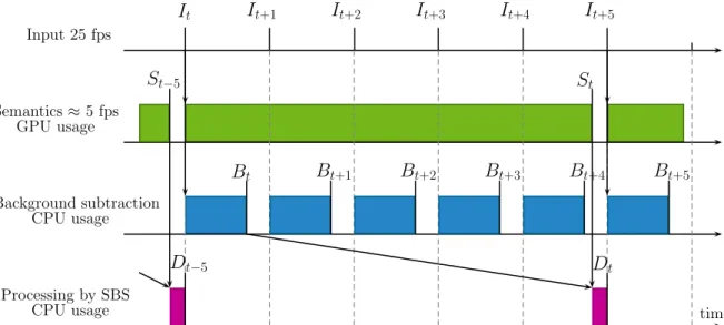
Problem Statement 69

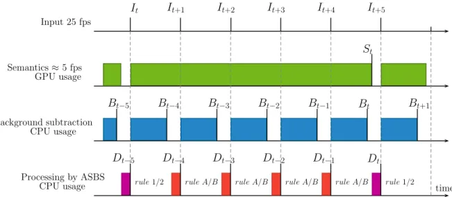
To better understand the problem, let us analyze the timing diagram of SBS, as displayed in 70

Figure1. For this time analysis, we assume that a GPU is used for semantic segmentation, and a CPU 71

is used for both the BGS algorithm and the SBS method. When the GPU is available, it starts analyzing 72

the input frame, otherwise it skips it. In the scenario of a BGS algorithm being faster than the semantic 73

segmentation network, which is the scenario that we examine in this paper, the BGS algorithm starts as 74

soon as the previous processing is over. The CPU then waits until semantics has been computed and a 75

semantic frame Stis available. The timeline analysis of SBS shows that: (1) with respect to the input 76

frame, the output frame is delayed by the time to compute semantics and to process the segmentation 77

map (this delay is unavoidable and constant), and (2) the output frame rate is mainly driven by the 78

slowest operation. It results that some output frames would be skipped, although the CPU computes 79

all the intermediate masks by the BGS algorithm. For example, in the case of Figure1, it is possible to 80

apply the BGS algorithm to It+2, but not to process Bt+2with the help of semantics. In other words, 81

the slowest operation dictates its rhythm (expressed in terms of frame rate) to the entire processing 82

chain. Hence, the semantics and the output have equal frame rates. This is not a problem as long as the 83

output frame rate (or equivalently that of semantics) is faster than the input frame rate. However, the 84

Input 25 fps Semantics ≈ 5 fps GPU usage Background subtraction CPU usage Processing by SBS CPU usage

I

I

I

I

I

I

S

B

D

D

B

S

B

B

B

B

Figure 1.Timing diagram of a naive real-time implementation of the semantic background subtraction (SBS) method when the frame rate of semantics is too slow to handle all the frames in real time. From top to bottom, the time lines represent: the input frames It, the computation of semantics Stby the

semantic segmentation algorithm (on GPU), the computation of intermediate segmentation masks Bt

by the BGS algorithm (on CPU), and the computation of output segmentation masks Dtby the SBS

method (on CPU). Vertical lines indicate when an image is available and filled rectangular areas display when a GPU or CPU performs a task. Arrows show the inputs required by the different tasks. This diagram shows that even when the background subtraction algorithm is real time with respect to the input frame rate, it is the computation of semantics that dictates the output frame rate.

Table 1.Comparison of the best mean F1score achieved for two semantic networks used in combination

with SBS on the CDNet 2014 dataset. These performances are obtained considering the SBS method, where the output of the BGS algorithm is replaced by the ground-truth masks. This indicates how the semantic information used in SBS would deteriorate a perfect BGS algorithm.

Networks SBS with PSPNet [25] SBS with MaskRCNN [26]

Best mean F1 0.953 0.674

semantics frame rate is generally slower than the input frame rate, which means that it is not possible 85

to process the video at its full frame rate, or in order words, that the processing of SBS is not real time. 86

To increase the output frame rate to its nominal value, we need to either accelerate the production 87

of semantics, which induces the choice of a faster but less accurate semantic network, or to interpolate 88

the missing semantics. Our analysis on semantic networks showed that faster networks are not 89

exploitable because of their lack of precision. Also, semantic segmentation networks should be 90

preferred to instance segmentation networks. For example, we had to discard MaskRCNN [26] and 91

prefer the PSPNet network [25], as shown in Table1. An alternative option is to interpolate missing 92

semantics. Naive ideas would be to skip the SBS processing step in the absence of semantics or to 93

repeat the last pixelwise semantic information when it is missing. Both ideas proved unsuccessful, 94

as shown in our experiments (see Section4). A better idea is to avoid any mechanism that would 95

substitute itself to the difficult calculation of semantics and, instead, replicate the decisions enforced 96

previously with the help of semantics to compensate for the lack of semantics later on. The underlying 97

question is whether or not we should trust and repeat decisions taken by SBS [30]. This idea has already 98

been applied in one of our recent work, called Real-time Semantic Background Subtraction [31] (noted 99

RT-SBS) with ViBe, a real-time BGS algorithm, and forms the basis of our new method, ASBS. This 100

paper presents our method in a complementary way to the original paper, with further experiments 101

and generalizes it to all background subtraction algorithms, including non-real-time ones. 102

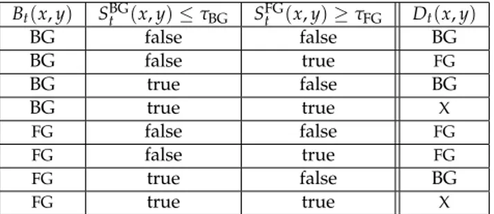
Table 2.Decision table as implemented by SBS. Rows corresponding to “don’t-care” values (X) cannot be encountered, assuming that τBG<τFG.

Bt(x, y) SBGt (x, y) ≤τBG SFGt (x, y) ≥τFG Dt(x, y) BG false false BG BG false true FG BG true false BG BG true true X FG false false FG FG false true FG FG true false BG FG true true X

The paper is organized as follows. Section2describes the semantic background subtraction (SBS) 103

method that underpins our developments. In Section3, we first discuss the classification problem of 104

background subtraction and take into account the specificities of semantics. Then, we describe our 105

new method. Experimental results are provided in Section4, and compared with those of the original 106

semantic background subtraction method when semantics is missing for some frames. Finally, we 107

conclude in Section5. 108

Contributions.We summarize our contributions as follows. (i) We propose a novel method, called 109

ASBS, for the task of background subtraction. (ii) We alleviate the problem of the slow computation of 110

semantics by substituting it for some frames with the help of a change detection algorithm. This makes 111

our method usable in real time. (iii) We show that at a semantic framerate corresponding to real-time 112

computations, we achieve results close to that of SBS, meaning that our substitute for semantics is 113

adequate. (iv) We show that our method ASBS with a real-time BGS algorithm such as ViBe and a 114

simple feedback mechanism achieves performances close to the ones of non real-time state-of-the-art 115

BGS algorithms such as SuBSENSE, while satisfying the real-time constraint. 116

2. Description of the semantic background subtraction method

117

Semantic background subtraction (SBS) [30,32] is a method based on semantics provided by deep 118

segmentation networks that enriches the pixel-wise decisions of a background subtraction algorithm. 119

In this section, we detail how SBS uses semantics to improve the classification of a BGS algorithm. 120

This description is necessary as SBS underpins our strategy to improve background subtraction in the 121

absence of semantics for some frames. 122

SBS combines three results at each pixel (x, y): the original classification result between 123

background (BG) and foreground (FG) at time t, as produced by a chosen BGS algorithm, denoted 124

by Bt ∈ {BG, FG}, and two booleans based on the semantic signals SBGt ∈ [0, 1]and SFGt ∈ [−1, 1], 125

derived from a semantic probability estimate defined hereinafter. These results are then combined to 126

output the final result Dt∈ {BG, FG}, as detailed in Table2. 127

The two semantic signals (SBG_t and S_tFG) are derived from a semantic probability estimate at each 128

pixel location, denoted by pS,t(x, y). This value is an estimate of the probability that pixel(x, y)belongs 129

to one of the objects contained in a set of potentially moving objects (person, car, etc) and depends 130

on the segmentation network itself. The authors of [30] use the PSPNet [25] semantic segmentation 131

network and compute pS,t(x, y)by applying a softmax function on the vector of output scores for this 132

pixel and add up the obtained values for the subset of classes of interest (see Section4.1for more 133

implementation details). 134

The first semantic signal, SBG_t (x, y), is the semantic probability estimate itself: SBG_t (x, y) =

interest for that pixel. According to rule 1, if this signal is lower than a threshold τBG, the pixel is labeled as background:

rule 1 : if SBGt (x, y) ≤τBG, then Dt(x, y) ←BG . (1) A convenient interpretation of rule 1 is that when it is activated (that is, when the condition is true), the 135

decision of the BGS algorithm is shadowed. Consequently, the amount of false positives (pixels wrongly 136

classified in the foreground), typically generated by illumination changes, dynamic backgrounds or 137

the presence of ghosts, is reduced since the semantic segmentation is unaffected by these well-known 138

BGS problems. 139

The second semantic signal, SFG_t (x, y), aims at improving the detection of foreground objects by detecting a local increase of the semantic probability estimate compared to a semantic background model, denoted by Mt. The signal SFG_t is calculated as the difference between the current semantic probability estimate and the value stored in the semantic background model:

SFGt (x, y) =pS,t(x, y) −Mt(x, y), (2) where the semantic background model Mtis initialized via:

M0(x, y) ← pS,0(x, y), (3)

and is possibly updated for each pixel only if the pixel is classified as belonging to the background: if Dt(x, y) =BG, thenα Mt+1(x, y) ← pS,t(x, y), (4) with the expression “if A thenα B” meaning that action B is applied with a probability α if condition A

is true. The goal for Mt(x, y)is to store the semantic probability estimate of the background in that pixel. When the value of SFG_t (x, y)is large, a jump in the semantic probability estimate for pixel(x, y)

is observed, and we activate rule 2 as defined by:

rule 2 : if SFGt (x, y) ≥τFG, then Dt(x, y) ←FG , (5) where τFGis a second positive threshold.

140

Again, when the condition of rule 2 is fulfilled, the result of the BGS algorithm is shadowed. 141

This second rule aims at reducing the number of missing foreground detections, for example when 142

a foreground object and the background appear to have similar colors (this is known as the color 143

camouflage effect). Note that, with a proper choice of threshold values τBG < τFG, both rules are 144

fully compatible meaning that they are never activated simultaneously. This relates to the “don’t-care” 145

situations described in Table2. 146

The decision table of Table2also shows that, when none of the two rules are activated, we use the result of the companion BGS algorithm as a fallback decision:

fallback : Dt(x, y) ←Bt(x, y). (6) 3. Asynchronous semantic background subtraction

147

To combine the output of any background subtraction to semantics according to SBS in real 148

time, it is necessary to calculate semantics at least at the same frame rate as the input video or BGS 149

stream, which is currently not achievable with high performances on any kind of videos, even on a 150

GPU. Instead of lowering the frame rate or reducing the image size, an alternative possibility consists 151

to interpolate missing semantics. Naive ideas, such as skipping the combination step of SBS in the 152

absence of semantics or repeating the last pixelwise semantic information when it is missing, have 153

proved unsuccessful, as shown in our experiments (see Section4). Hence, it is better to find a substitute 154

for missing semantics. Obviously, it is unrealistic to find a substitute that would be as powerful as 155

full semantics while being faster to calculate. Instead, we propose to replicate the decisions enforced 156

previously with the help of semantics to compensate for the lack of semantics later on. The underlying 157

question is whether or not we should trust and repeat decisions taken by SBS [30]. This idea is the 158

basis of our new method. 159

The cornerstone for coping with missing semantics is the fact that the true class (foreground or 160

background) of a pixel generally remains unchanged between consecutive video frames, as long as 161

the object in that pixel remains static. It is therefore reasonable to assume that if a correct decision 162

is enforced with the help of semantics for a given pixel location and video frame, the same decision 163

should be taken in that pixel location for the subsequent frames (when semantics is not computed) 164

if the features of that pixel appear to be unchanged. Our method, named Asynchronous Semantic 165

Background Subtraction (ASBS), thus consists in interpolating the decisions of SBS by memorizing 166

information about the activation of rules as well as the pixel features, which we chose to be the input 167

color in our case, when semantics is computed (SBS is then applied), and copying the decision of the 168

last memorized rule when semantics is not computed if the color remains similar (which tends to 169

indicate that the object is the same). 170

To further describe ASBS, let us first focus on a substitute for rule 1, denoted rule A hereafter, 171

that replaces rule 1 in the absence of semantics. If rule 1 was previously activated in pixel(x, y)while 172

the current color has remained similar, then Dt(x, y)should be set to the background. To enable this 173

mechanism, we have to store, in a rule map denoted by R, if rule 1 of SBS is activated; this is indicated 174

by R(x, y)←1. Simultaneously, we memorize the color of that pixel in a color map, denoted by C. With 175

these components, rule A becomes: 176

rule A : if R(x, y) =1 and dist(C(x, y), It(x, y)) ≤τA,

then Dt(x, y) ←BG , (7)

where τA is a fixed threshold applied on the Manhattan (or Euclidean) distance between the color 177

C(x, y)stored in the color map and the input color It(x, y). Theoretically, it is also possible to refine the 178

color model by adopting a model used by a BGS algorithm in which case the distance function should 179

be chosen accordingly; our choice to favor a simple model instead proved effective. 180

Likewise, we can replace rule 2 by rule B in the absence of semantics. When rule 2 is activated, 181

this decision is stored in the rule map (this is indicated by R(x, y)←2), and the color of the pixel is 182

stored in the color map C. Rule B thus becomes: 183

rule B : if R(x, y) =2 and dist(C(x, y), It(x, y)) ≤τB,

then Dt(x, y) ←FG . (8)

where τBis a second threshold. Again, when neither rule A nor rule B are activated, the BGS decision 184

is used as a fallback decision. 185

The updates of the rules and color map are detailed in Algorithm1. It is an add-on for SBS that 186

memorizes decisions and colors based on computed semantics upon activation of a rule. The second 187

component of ASBS, described in Algorithm2, is the application of rule A, rule B, or the fallback 188

decision, when no semantics is available. 189

Note that the two pseudo-codes, which define pixel-wise operations, could be applied within 190

the same video frame if the semantics was only computed inside a specific region-of-interest. In 191

that scenario, we would apply the pseudo-code of Algorithm2for pixels without semantics and 192

the pseudo-code of Algorithm1for pixels with semantics. It is therefore straightforward to adapt 193

the method from a temporal sub-sampling to a spatial sub-sampling, or to a combination of both. 194

However, a typical setup is that semantics is computed for the whole frame and is skipped for the next 195

few frames at a regular basis. In section4, we evaluate ASBS for this temporal sub-sampling since it 196

Figure 2. Schematic representation of our method named ASBS, extending SBS [30], capable to combine the two asynchronous streams of semantics and background subtraction masks to improve the performances of BGS algorithms. When semantics is available, ASBS applies Rule 1, Rule 2, or selects the fallback, and it updates the color and rule maps. Otherwise, ASBS applies Rule A, Rule B, or it selects the fallback.

Algorithm 1Pseudo-code of ASBS for pixels with semantics. The rule and color maps are updated during the application of SBS (note that R is initialized with zero values at the program start).

Require: Itis the input color frame (at time t) 1: for all(x, y)with semantics do

2: Dt(x, y) ←apply SBS in(x, y) 3: ifrule 1 was activated then 4: R(x, y) ←1

5: C(x, y) ← It(x, y)

6: else ifrule 2 was activated then 7: R(x, y) ←2 8: C(x, y) ← It(x, y) 9: else 10: R(x, y) ←0 11: end if 12: end for

Algorithm 2 Pseudo-code of ASBS for pixels without semantics, rule A, rule B or the fallback are applied.

Require: Itis the input color frame (at time t) 1: for all(x, y)without semantics do

2: if R(x, y) =1 then 3: ifdist(C(x, y), It(x, y)) ≤τAthen 4: Dt(x, y) ←BG 5: end if 6: else if R(x, y) =2 then 7: ifdist(C(x, y), It(x, y))) ≤τBthen 8: Dt(x, y) ←FG 9: end if 10: else 11: Dt(x, y) ←Bt(x, y) 12: end if 13: end for

has a unique implementation, while spatial sub-sampling can involve complex strategies for choosing 197

the regions where to compute the semantics and is application-dependent anyway. Our method, 198

illustrated in Figure2for the case of entire missing semantic frames, is applicable in combination with 199

virtually any BGS algorithm. 200

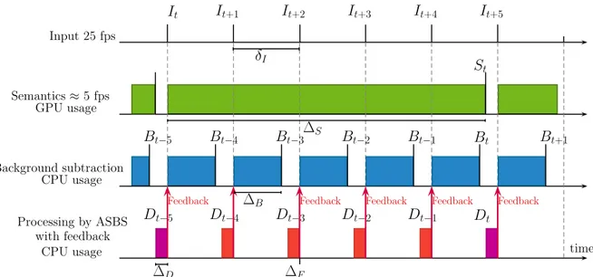
Timing diagrams of ASBS 201

The ASBS method introduces a small computational overhead (a distance has to be computed 202

for some pixels) and memory increase (a rule map and a color map are memorized). However, these 203

overheads are negligible with respect to the computation of semantics. The practical benefits of ASBS 204

can be visualized on a detailed timing diagram of its components. For a formal discussion, we use the 205

following notations: 206

• It, St, Bt, Dtrespectively denote an arbitrary input, semantics, background segmented by the 207

BGS algorithm, and the background segmented by ASBS, indexed by t. 208

• δIrepresents the time between two consecutive input frames. 209

• ∆_S,∆B,∆Dare the times needed to calculate the semantics, the BGS output, and to apply SBS or 210

ASBS, which are supposed to be the same, respectively. These times are reasonably constant. 211

Input 25 fps Semantics ≈ 5 fps GPU usage Background subtraction CPU usage Processing by ASBS CPU usage

It

It+1

It+2

It+3

It+4

It+5

St

B

D

D

B

D

D

D

D

B

B

B

Bt

rule 1/2 rule A/B rule A/B rule A/B rule A/B rule 1/2

Bt+1

Figure 3.Timing diagram of ASBS in the case of a real-time BGS algorithm (∆B<δI) satisfying the

condition∆B+∆D <δI. Note that the output stream is delayed by a constant∆S+∆Dtime with

respect to the input stream.

We assume that semantics is calculated on a GPU, whereas the BGS and the application of the rules are 212

calculated on a single threaded CPU hardware. Also, the frame rate of semantics is supposed to be 213

smaller than that of BGS; that is∆S>∆B. 214

We now examine two different scenarios. The first scenario is that of a real-time BGS algorithm 215

(∆B<δI) satisfying the condition∆B+∆D<δI. This scenario, illustrated in Figure3, can be obtained 216

with the ViBe [5] BGS algorithm for example; this scenario is further described in [31]. On the timing 217

diagram, it can be seen that the output frame rate is then equal to the input frame rate, all frames being 218

segmented either by SBS (rule 1/2) or ASBS (rule A/B) with a time delay corresponding approximately 219

to∆S. We present illustrative numbers for this timing diagram in Section4.4. 220

In a second scenario, the frame rate of the BGS is too slow to accommodate to real time with 221

ASBS. It means that∆B+∆D>δI. In this case, the output frame rate is mainly dictated by∆B, since 222

∆B >> ∆D. The input frame rate can then be viewed as slowed down by the BGS algorithm, in 223

which case the timing diagrams fall back to the same case as a real-time BGS algorithm by artificially 224

changing δIto ˜δI, where ˜δI=∆B+∆D>δI. It is a scenario that, unfortunately, follows the current 225

trend to produce better BGS algorithms at the price of more complexity and lower processing frame 226

rates. Indeed, according to our experiments and [33], the top unsupervised BGS algorithms ranked on 227

the CDNet web site (seehttp://changedetection.net) are not real time. 228

4. Experimental results

229

In this section, we evaluate the performances of our novel method ASBS and compare them to 230

those of the original BGS algorithm and those of the original SBS method [30]. First, in Section4.1, we 231

present our evaluation methodology. This comprises the choice of a dataset along with the evaluation 232

metric, and all needed implementation details about ASBS, such as how we compute the semantics, 233

and how we choose the values of the different thresholds. In Section4.2, we evaluate ASBS when 234

combined with state-of-the-art BGS algorithms. Section4.3is devoted to a possible variant of ASBS 235

which includes a feedback mechanism that can be applied to any conservative BGS algorithm. Finally, 236

we discuss the computation time of ASBS in Section4.4. 237

4.1. Evaluation methodology 238

For the quantitative evaluation, we chose the CDNet 2014 dataset [12] which is composed of 53 239

video sequences taken in various environmental conditions such as bad weather, dynamic backgrounds 240

and night conditions, as well as different video acquisition conditions, such as PTZ and low frame rate 241

cameras. This challenging dataset is largely employed within the background subtraction community 242

and currently serves as the reference dataset to compare state-the-art BGS techniques. 243

We compare performances on this dataset according to the overall F1score, which is one of the 244

most widely used performance scores for this dataset. For each video, F1is computed by: 245

F1=

2TP

2TP+FP+FN, (9)

where TP (true positives) is the number of foreground pixels correctly classified, FP (false positives) the 246

number of background pixels incorrectly classified, and FN (false negatives) the number of foreground 247

pixels incorrectly classified. The overall F1score on the entire dataset is obtained by first averaging 248

the F1 scores over the videos, then over the categories, according the common practice of CDNet [12]. 249

Note that this averaging introduces inconsistencies between overall scores that can be avoided by 250

using summarization instead, as described in [34], but to allow a fair comparison with the other BGS 251

algorithms, we decided to stick to the original practice of [12] for our experiments. 252

We compute the semantics as in [30], that is with the semantic segmentation network PSPNet [25] 253

trained on the ADE20K dataset [35] (using the public implementation [36]). The network outputs a 254

vector containing 150 real numbers for each pixel, where each number is associated to a particular 255

object class within a set of 150 mutually exclusive classes. The semantic probability estimate pS,t(x, y) 256

is computed by applying a softmax function to this vector and summing the values obtained for classes 257

that belong to a subset of classes that are relevant for motion detection. We use the same subset of 258

classes as in [30] (person, car, cushion, box, boot, boat, bus, truck, bottle, van, bag and bicycle), whose 259

elements correspond to moving objects of the CDNet 2014 dataset. 260

For dealing with missing semantics, since the possibilities to combine spatial and temporal 261

sampling schemes are endless, we have restricted the study to the case of a temporal sub-sampling of 262

one semantic frame per X original frames; this sub-sampling factor is referred to as X:1 hereafter. In 263

other scenarios, semantics could be obtained at a variable frame rate or for some variable regions of 264

interest, or even a mix of these sub-sampling schemes. 265

The four thresholds are chosen as follows. For each BGS algorithm, we optimize the thresholds 266

(τBG, τFG)of SBS with a grid search to maximize its overall F1score. Then, in a second time, we freeze 267

the optimal thresholds(τ_BG∗ , τ_FG∗ )found by the first grid search and optimize the thresholds(τA, τB)of 268

ASBS by a second grid search for each pair (BGS algorithm, X:1), to maximize the overall F1score once 269

again. Such methodology allows a fair comparison between SBS and ASBS as the two techniques use 270

the same common parameters(τ_BG∗ , τ_FG∗ )and ASBS is compared to an optimal SBS method. Note that 271

the α parameter is chosen as in [30]. 272

The segmentation maps of the BGS algorithms are either taken directly from the CDNet 2014 273

website (when no feedback mechanism is applied) or computed using the public implementations 274

available at [37] for ViBe [5] and [38] for SuBSENSE [6] (when the feedback mechanism of Section4.3 275

is applied). 276

4.2. Performances of ASBS 277

A comparison of the performances obtained with SBS and ASBS for four state-of-the-art BGS 278

algorithms (IUTIS-5 [8], PAWCS [7], SuBSENSE [6], and WebSamBe [39]) and for different sub-sampling 279

factors is provided in Figure4. For the comparison with SBS, we used two naive heuristics for dealing 280

with missing semantic frame as, otherwise, the evaluation would be done on a subset of the original 281

images as illustrated in Figure1. The first heuristic simply copies Btin Dtfor frames with missing 282

semantics. The second heuristic uses the last available semantic frame Stin order to still apply rule 1 283

and rule 2 even when no up-to-date semantic frames are available. Let us note that this last naive 284

heuristic corresponds to using ASBS with τAand τBchosen big enough so that the condition on the 285

color of each pixel is always satisfied. 286

1 5 10 15 20 25 0.78 0.79 0.8 0.81 Overall F1 IUTIS-5 [8] 1 5 10 15 20 25 0.75 0.76 0.77 0.78 PAWCS [7] 1 5 10 15 20 25 0.74 0.75 0.76 0.77 0.78 0.79

Temporal sub-sampling factor X:1

Overall F1 SuBSENSE [6] 1 5 10 15 20 25 0.75 0.76 0.77 0.78 0.79

Temporal sub-sampling factor X:1 WeSamBe [39]

Original BGS SBS (with copy of Bt) SBS (with copy of St) ASBS without feedback

Figure 4.Overall F1scores obtained with SBS and ASBS for four state-of-the-art BGS algorithms and

different sub-sampling factors. The performances of ASBS decrease much more slowly than those of SBS with the decrease of the semantic frame rate and, therefore, are much closer to those of the ideal case (SBS with all semantic maps computed, that is SBS 1:1), meaning that ASBS provides better decisions for frames without semantics. On average, ASBS with 1 frame of semantics out of 25 frames (ASBS 25:1) performs as well as SBS, with copy of Bt, with 1 frame of semantics out of 2 frames (SBS

2:1).

As can be seen, the performances of ASBS decrease much more slowly than those of SBS with the 287

decrease of the semantic frame rate and, therefore, are much closer to those of the ideal case (SBS with 288

all semantic maps computed, that is SBS 1:1), meaning that ASBS provides better decisions for frames 289

without semantics. 290

A second observation can be made concerning the heuristic repeating St. The performances 291

become worse than the ones of the original BGS for semantic frame rates lower than 1 out of 5 292

frames, but they are better than SBS when repeating Btfor high semantic frame rates. This observation 293

emphasizes the importance of checking the color feature as done with ASBS instead of blindly repeating 294

the corrections induced by semantics. The performances for lower frame rates are not represented 295

for the sake of figure clarity but still decrease linearly to very low performances. For example, in the 296

case of IUTIS_5, the performance drops to 0.67 at 25:1. In the rest of the paper, when talking about 297

performances on SBS at different frame rates, we only consider the heuristic where we copy Btas it is 298

the one that behaves the best, given our experimental setup. Finally, it can be seen that, on average, 299

ASBS with 1 frame of semantics out of 25 frames (ASBS 25:1) performs as well as SBS, with copy of Bt, 300

with 1 frame of semantics out of 2 frames (SBS 2:1). 301

In Figure5, we also compare the effects of SBS with copied Btin Dtfor frames with missing 302

semantics, and ASBS for different BGS algorithms by looking at their performances in the mean 303

ROC space of CDNet 2014 (ROC space where the false and true foreground rates are computed 304

(a) SBS at 5:1 (b) ASBS at 5:1 (ours) Figure 5.Effects of SBS and ASBS on BGS algorithms in the mean ROC space of CDNet 2014 [12]. Each point represents the performance of a BGS algorithm and the end of the associated arrow indicates the performance after application of the methods for a temporal sub-sampling factor of 5:1. We observe that SBS improves the performances, but only marginally, whereas ASBS moves the performances much closer to the oracle (upper left corner).

according to the rules of [12]). The points represent the performances of different BGS algorithms 305

whose segmentation maps can be downloaded on the dataset website. The arrows represent the effects 306

of SBS and ASBS for a temporal sub-sampling factor of 5:1. This choice of frame rate is motivated by 307

the fact that it is the frame rate at which PSPNet can produce the segmentation maps on a GeForce 308

GTX Titan X GPU. We observe that SBS improves the performances, but only marginally, whereas 309

ASBS moves the performances much closer to the oracle (upper left corner). 310

To better appreciate the positive impact of our strategy for replacing semantics, we also provide a 311

comparative analysis of the F1score by only considering the frames without semantics. We evaluate 312

the relative improvement of the F1score of ASBS, SBS and the second heuristic (SBS with copies of 313

St) compared to the original BGS algorithm (which is equivalent to the first heuristic, SBS with copies 314

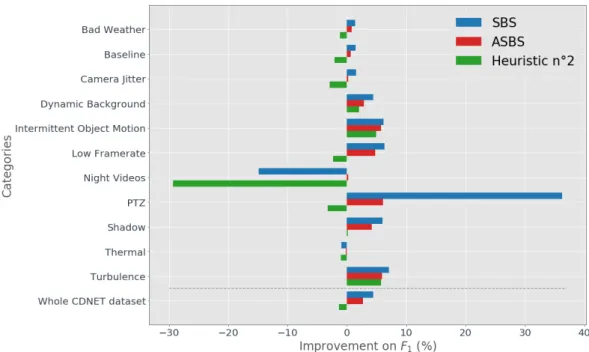
of Bt). In Figure6, we present our analysis on a per-category basis, in the same fashion as in [30]. As 315

shown, the performances of ASBS are close to the ones of SBS for almost all categories, indicating 316

that our substitute for semantics is adequate. We can also observe that the second heuristic does not 317

perform well, and often degrades the results compared the original BGS algorithm. In this Figure, SBS 318

appears to fail for two categories: “night videos” and “thermal”. This results from the ineffectiveness 319

of PSPNet to process videos of these categories, as this network is not trained with such image types. 320

Interestingly, ASBS is less impacted than SBS because it refrains from copying some wrong decisions 321

enforced by semantics. 322

Finally, in Figure 7, we provide the evolution of the optimal parameters τA and τB with 323

the temporal sub-sampling factor (in the case of PAWCS). The optimal value decreases with the 324

sub-sampling factor, implying that the matching condition on colors become tighter or, in other 325

words, that rule A and rule B should be activated less frequently for lower semantic frame rates, as a 326

consequence of the presence of more outdated colors in the color map for further images. 327

4.3. A feedback mechanism for SBS and ASBS 328

The methods SBS and ASBS are designed to be combined to a BGS algorithm to improve the 329

quality of the final segmentation, but they do not affect the decisions taken by the BGS algorithm itself. 330

In this section, we explore possibilities to embed semantics inside the BGS algorithm itself, which 331

would remain blind to semantics otherwise. Obviously, this requires to craft modifications specific to a 332

particular algorithm or family of algorithms, which can be effortful as explained hereinafter. 333

Figure 6.Per-category analysis. We display the relative improvements of the F1score of SBS, ASBS, and

the second heuristic compared with the original algorithms, by considering only the frames without semantics (at a 5:1 semantic frame rate).

5 10 15 20 25 5 25 45 65 85 105

Temporal sub-sampling factor X:1

Optimal

value

Evolution of the optimal values of τAand τB

τA τB

Figure 7.Evolution of the optimal thresholds τAand τBof the ASBS method when the semantic frame

rate is reduced. Note that the Manhattan distance associated to these thresholds is computed on 8-bit color values. The results are shown here for the PAWCS algorithm, and follow the same trend for the other BGS algorithms considered in Figure4.

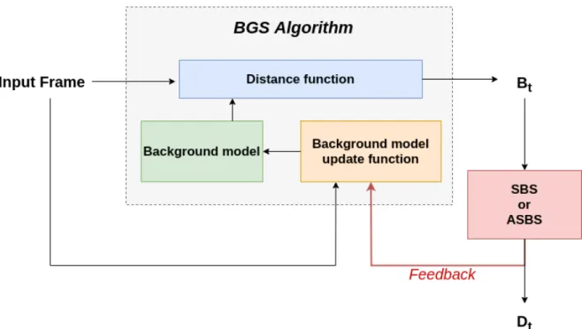
Figure 8.Our feedback mechanism, which impacts the decisions of any BGS algorithm whose model update is conservative, consists to replace the BG/FG segmentation of the BGS algorithm by the final segmentation map improved by semantics (either by SBS or ASBS) to update the internal background model.

The backbone of many BGS algorithms is composed of three main parts. First, an internal model 334

of the background is kept in memory, for instance in the form of color samples or other types of 335

features. Second, the input frame is compared to this model via a distance function to classify pixels as 336

background or foreground. Third, the background model is updated to account for changes in the 337

background over time. 338

A first possibility to embed semantics inside the BGS algorithm is to include semantics directly 339

in a joint background model integrating color and semantic features. This requires to formulate the 340

relationships that could exist between them and to design a distance function accounting for these 341

relationships, which is not trivial. Therefore, we propose a second way of doing so by incorporating 342

semantics during the update, which is straightforward for algorithms whose model updating policy is 343

conservative (as introduced in [5]). For those algorithms, the background model in pixel(x, y)may 344

be updated if Bt(x, y) = BG, but it is always left unchanged if Bt(x, y) = FG, which prevents the 345

background model from being corrupted with foreground features. In other words, the segmentation 346

map Btserves as an updating mask. As Dtproduced by SBS or ASBS is an improved version of Bt, we 347

can advantageously use Dtinstead of Btto update the background model, as illustrated in Figure8. 348

This introduces a semantic feedback which improves the internal background model and, consequently, 349

the next segmentation map Bt+1, whether or not semantics is computed. 350

To appreciate the benefit of a semantic feedback, we performed experiments for two well-known 351

conservative BGS algorithms, ViBe and SuBSENSE, using the code made available by the authors (see 352

[37] for ViBe and [38] for SuBSENSE). Let us note that the performances for SuBSENSE are slightly 353

lower than the ones reported in Figure4as there are small discrepancies between the performance 354

reported on the CDNet web site and the ones obtained with the available source code. 355

Figure9(left column) reports the results of ASBS with the feedback mechanism on ViBe and 356

SuBSENSE, and compares them to the original algorithm and the SBS method. Two main observations 357

can be made. First, as for the results of the previous section, SBS and ASBS both improve the 358

performances even when the semantic frame rate is low. Also, ASBS always performs better. Second, 359

5 10 15 20 25 0.6 0.65 0.7 0.75 Mean F1

ViBe + ASBS with feedback evaluated on Dt

5 10 15 20 25

0.6 0.65 0.7 0.75

ViBe + ASBS with feedback evaluated on Bt

5 10 15 20 25

0.73 0.75 0.78

Temporal sub-sampling factor X:1

Mean

F1

SuBSENSE + ASBS with feedback evaluated on Dt

5 10 15 20 25

0.73 0.75 0.78

Temporal sub-sampling factor X:1 SuBSENSE + ASBS with feedback evaluated on Bt

Original BGS SBS Feedback ASBS without feedback ASBS with feedback Figure 9.Comparison of the performances, computed with the mean F1score on the CDNet 2014, of

SBS and ASBS when there is a feedback that uses Dtto update the model of the BGS algorithm. The

results are given with respect to a decreasing semantic frame rate. It can be seen that SBS and ASBS always improve the results of the original BGS algorithm and that a feedback is beneficial. Graphs in the right column show that the intrinsic quality of the BGS algorithms is improved, as their output Bt,

prior to any combination with semantics, produces higher mean F1scores.

including the feedback always improves the performances for both SBS and ASBS, and for both BGS 360

algorithms. In the case of ViBe, the performance is much better when the feedback is included. For 361

SuBSENSE, the performance is also improved, but only marginally. This might be due to the fact 362

that ViBe has a very straightforward way of computing the update of the background model while 363

SuBSENSE uses varying internal parameters and heuristics, calculated adaptively. It is thus more 364

difficult to interpret the impact of a better updating map on SuBSENSE than it is on ViBe. 365

We also investigated to what extend the feedback provides better updating maps to the BGS 366

algorithm. For conservative algorithms, this means that, internally, the background model is built with 367

better features. This measure can be evaluated using the output of the classification map, Bt. 368

For that purpose, we compared the original BGS algorithm and the direct output, that is Btin 369

Figure8, of the feedback method when the updating map is replaced by Dtobtained by either SBS or 370

ASBS. As can be seen in Figure9(right column), using the semantic feedback always improves the 371

BGS algorithm whether the updating map is obtained from SBS or ASBS. This means that the internal 372

background model of the BGS algorithm is always enhanced and that, consequently, a feedback helps 373

the BGS algorithm to take better decisions. 374

Finally, let us note that ViBe, which is a real-time BGS algorithm, combined with semantics 375

provided at a real-time rate (about 1 out of 5 frames) and with the feedback from ASBS has a mean F1 376

performance of 0.746, which is the same performance as the original SuBSENSE algorithm (0.746) that 377

is not real time [33]. This performance corresponds to the performance of RT-SBS presented in [31]. 378

Table 3.Mean computation time∆D(ms/frame) of SBS and ASBS.

∆D(SBS) 1.56

∆D(ASBS : frames with semantics) 2.12

∆D(ASBS : frames without semantics) 0.8

It can be seen that our method can thus help real-time algorithms to reach performances of the top 379

unsupervised BGS algorithms while meeting the real-time constraint, which is a huge advantage in 380

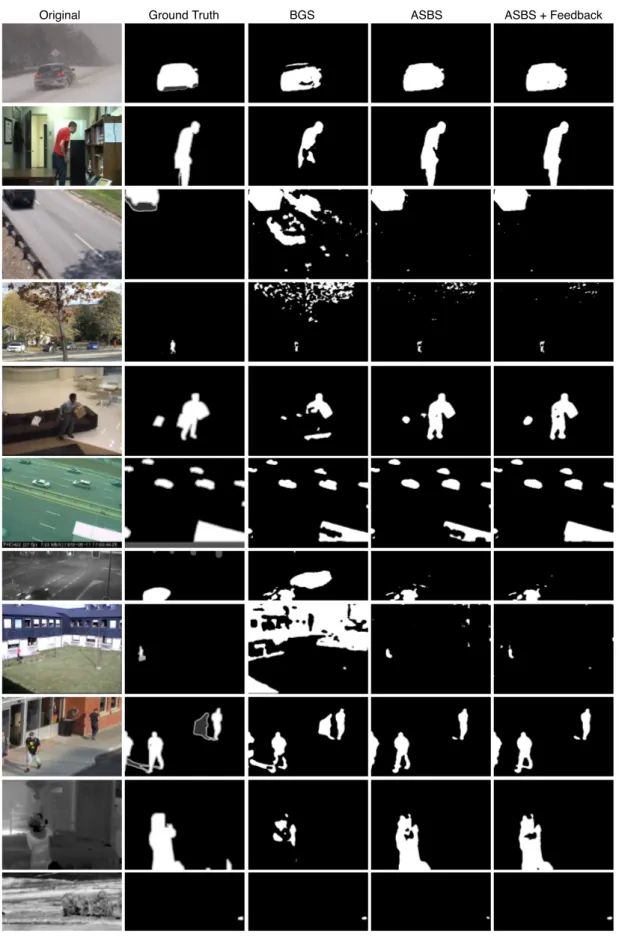
practice. We illustrate our two novel methods, ASBS and the feedback, in Figure10on one video of 381

each category of the CDNet2014 dataset using ViBe as BGS algorithm. 382

One last possible refinement would consist to adapt the updating rate of the background model 383

according to a rule map similar to that of ASBS. More specifically, if Bt(x, y) =FG and Dt(x, y) =BG, 384

we could assume that the internal background model in pixel(x, y)is inadequate and, consequently, we 385

could increase the updating rate in that pixel. Tests performed on ViBe showed that the performances 386

are improved with this strategy. However, this updating rate adaptation has to be tailored for each 387

BGS algorithm specifically; therefore, we did not consider this final refinement in our experiments. 388

We only evaluated the impact of the feedback mechanism on BGS algorithms with a conservative 389

updating policy, and avoided any particular refinement that would have biased the evaluation. 390

4.4. Time analysis of ASBS 391

In this section, we show the timing diagram of ASBS and provide typical values for the different 392

computation durations. 393

The timing diagram of ASBS with feedback is presented in Figure11. The inclusion of a feedback 394

has two effects. First, we need to include the feedback time∆Fin the time needed for the background 395

subtraction algorithm ∆B. In our case, as we only substitute the updating map by Dt, it can be 396

implemented as a simple pointer replacement and therefore∆Fis negligible (in the following, we take 397

∆F '0 ms). Second, we have to wait for the ASBS (or SBS) to finish before starting the background 398

subtraction of the next frame. 399

Concerning the computation time of BGS algorithms, Roy et al. [33] have provided a reliable 400

estimate of the processing speed of leading unsupervised background subtraction algorithms. They 401

show that the best performing ones are not real time. Only a handful of algorithms are actually real 402

time, such as ViBe that can operate at about 200 fps on CDNet 2014 dataset, that is∆B =5 ms. With 403

PSPNet, the semantic frame rate is of about 5 to 7 fps for a NVIDIA GeForce GTX Titan X GPU, which 404

corresponds to∆S'200 ms. It means that for 25 fps videos, we have access to semantics about once 405

every 4 to 5 frames. In addition, Table3reports our observation about the mean execution time per 406

frame of∆Dfor SBS and ASBS. These last tests were performed on a single thread running on a single 407

processor Intel(R) Xeon(X) E5-2698 v4 2.20GHz. 408

Thus, in the case of ViBe, we start from a frame rate of about 200 fps in its original version to 409

reach about 160 fps when using ASBS, which is still real time. This is important because, as shown 410

in Section4.3, the performances of ViBe with ASBS at a semantic frame rate of 1 out of 5 frames and 411

feedback is the same as SuBSENSE that, alone, runs at a frame rate lower than 25 fps [33]. Hence, 412

thanks to ASBS, we can replace BGS algorithms that work well but are too complex to run in real time 413

and are often difficult to interpret by a combination of a much simpler BGS algorithm and a processing 414

based on semantics, regardless of the frame rate of the last. Furthermore, ASBS is much easier to 415

optimize as the parameters that we introduce are few in number and easy to interpret. In addition, 416

we could also fine-tune the semantics, by selecting a dedicated set of objects to be considered, for a 417

scene-specific setup. It is our belief that there are still some margins for further improvements. 418

Original Ground Truth BGS ASBS ASBS + Feedback

Figure 10. Illustration of the results of ASBS using ViBe as BGS algorithm. From left to right, we provide the original color image, the ground truth, the BGS as provided by the original ViBe algorithm, using our ASBS method without any feedback, and using ASBS and a feedback. Each line corresponds to a representative frame of a video in each category of CDNet2014.

Input 25 fps Semantics ≈ 5 fps GPU usage Background subtraction CPU usage Processing by ASBS CPU usage

I

I

I

I

I

I

S

B

D

D

B

D

D

D

D

B

B

B

B

B

Feedback

∆

∆

∆

∆

δ

Figure 11.Timing diagram of ASBS with a feedback mechanism in the case of a real-time BGS algorithm (∆B <δI) satisfying the condition∆B+∆D<δI and the computation of semantics being not real-time

(∆S>δI). Note that the feedback time∆Fis negligible.

5. Conclusion

419

In this paper, we presented a novel method, named ASBS, based on semantics for improving the 420

quality of segmentation masks produced by background subtraction algorithms when semantics is not 421

computed for all video frames. ASBS, which is derived from the semantic background subtraction 422

method, is applicable to any off-the-shelf background subtraction algorithm and introduces two new 423

rules in order to repeat semantic decisions, even when semantics and the background are computed 424

asynchronously. We also presented a feedback mechanism to update the background model with 425

better samples and thus take better decisions. We showed that ASBS improves the quality of the 426

segmentation masks compared to the original semantic background subtraction method applied only 427

to frames with semantics. Furthermore, ASBS is straightforward to implement and cheap in terms of 428

computation time and memory consumption. We also showed that applying ASBS with the feedback 429

mechanism allows to elevate an unsupervised real-time background subtraction algorithm to the 430

performance of non real-time state-of-the-art algorithms. 431

A more general conclusion is that, when semantics is missing for some frames but needed to 432

perform a task (in our case, the task of background subtraction), our method provides a convenient 433

and effective mechanism to interpolate the missing semantics. The mechanism of ASBS might thus 434

enable real-time computer vision tasks requiring semantic information. 435

Implementations of ASBS in the Python language for CPU and GPU are available at the following 436

addresshttps://github.com/cioppaanthony/rt-sbs. 437

Acknowledgment

438

A. Cioppa has a grant funded by the FRIA, Belgium. This work is part of a patent application (US 439

2019/0197696 A1). 440

441

1. Bouwmans, T. Traditional and recent approaches in background modeling for foreground detection: An 442

overview. Computer Science Review 2014, 11-12, 31–66. 443

2. Stauffer, C.; Grimson, E. Adaptive background mixture models for real-time tracking. IEEE International 444

Conference on Computer Vision and Pattern Recognition (CVPR); , 1999; Vol. 2, pp. 246–252. 445

3. Elgammal, A.; Harwood, D.; Davis, L. Non-parametric Model for Background Subtraction. European 446

Conference on Computer Vision (ECCV). Springer, 2000, Vol. 1843, Lecture Notes in Computer Science, pp. 447

751–767. 448

4. Maddalena, L.; Petrosino, A. A Self-Organizing Approach to Background Subtraction for Visual 449

Surveillance Applications. IEEE Transactions on Image Processing 2008, 17, 1168–1177. 450

5. Barnich, O.; Van Droogenbroeck, M. ViBe: A universal background subtraction algorithm for video 451

sequences. IEEE Transactions on Image Processing 2011, 20, 1709–1724. 452

6. St-Charles, P.L.; Bilodeau, G.A.; Bergevin, R. SuBSENSE: A Universal Change Detection Method with 453

Local Adaptive Sensitivity. IEEE Transactions on Image Processing 2015, 24, 359–373. 454

7. St-Charles, P.L.; Bilodeau, G.A.; Bergevin, R. Universal Background Subtraction Using Word Consensus 455

Models. IEEE Transactions on Image Processing 2016, 25, 4768–4781. 456

8. Bianco, S.; Ciocca, G.; Schettini, R. Combination of Video Change Detection Algorithms by Genetic 457

Programming. IEEE Transactions on Evolutionary Computation 2017, 21, 914–928. 458

9. Javed, S.; Mahmood, A.; Bouwmans, T.; Jung, S.K. Background-Foreground Modeling Based on 459

Spatiotemporal Sparse Subspace Clustering. IEEE Transactions on Image Processing 2017, 26, 5840–5854. 460

10. Ebadi, S.; Izquierdo, E. Foreground Segmentation with Tree-Structured Sparse RPCA. IEEE Transactions on 461

Pattern Analysis and Machine Intelligence 2018, 40, 2273–2280. 462

11. Vacavant, A.; Chateau, T.; Wilhelm, A.; Lequièvre, L. A Benchmark Dataset for Outdoor 463

Foreground/Background Extraction. Asian Conference on Computer Vision (ACCV). Springer, 2012, Vol. 464

7728, Lecture Notes in Computer Science, pp. 291–300. 465

12. Wang, Y.; Jodoin, P.M.; Porikli, F.; Konrad, J.; Benezeth, Y.; Ishwar, P. CDnet 2014: An Expanded Change 466

Detection Benchmark Dataset. IEEE International Conference on Computer Vision and Pattern Recognition 467

Workshops (CVPRW); , 2014; pp. 393–400. 468

13. Cuevas, C.; Yanez, E.; Garcia, N. Labeled dataset for integral evaluation of moving object detection 469

algorithms: LASIESTA. Computer Vision and Image Understanding 2016, 152, 103–117. 470

14. Braham, M.; Van Droogenbroeck, M. Deep Background Subtraction with Scene-Specific Convolutional 471

Neural Networks. IEEE International Conference on Systems, Signals and Image Processing (IWSSIP), 472

2016, pp. 1–4. 473

15. Bouwmans, T.; Garcia-Garcia, B. Background Subtraction in Real Applications: Challenges, Current 474

Models and Future Directions. CoRR 2019, abs/1901.03577. 475

16. Lim, L.; Keles, H. Foreground Segmentation Using Convolutional Neural Networks for Multiscale Feature 476

Encoding. Pattern Recognition Letters 2018, 112, 256–262. 477

17. Wang, Y.; Luo, Z.; Jodoin, P.M. Interactive Deep Learning Method for Segmenting Moving Objects. Pattern 478

Recognition Letters 2017, 96, 66–75. 479

18. Zheng, W.B.; Wang, K.F.; Wang, F.Y. Background Subtraction Algorithm With Bayesian Generative 480

Adversarial Networks. Acta Automatica Sinica 2018, 44, 878–890. 481

19. Babaee, M.; Dinh, D.; Rigoll, G. A Deep Convolutional Neural Network for Background Subtraction. 482

Pattern Recognition 2018, 76, 635–649. 483

20. Zhou, B.; Zhao, H.; Puig, X.; Fidler, S.; Barriuso, A.; Torralba, A. Scene Parsing through ADE20K Dataset. 484

IEEE International Conference on Computer Vision and Pattern Recognition (CVPR); , 2017; pp. 5122–5130. 485

21. Everingham, M.; Van Gool, L.; Williams, C.; Winn, J.; Zisserman, A. The PASCAL Visual Object 486

Classes Challenge 2012 (VOC2012) Results.http://www.pascal-network.org/challenges/VOC/voc2012/

487

workshop/index.html. 488

22. Cordts, M.; Omran, M.; Ramos, S.; Rehfeld, T.; Enzweiler, M.; Benenson, R.; Franke, U.; Roth, S.; Schiele, 489

B. The Cityscapes Dataset for Semantic Urban Scene Understanding. IEEE International Conference on 490

Computer Vision and Pattern Recognition (CVPR); , 2016; pp. 3213–3223. 491

23. Lin, T.Y.; Maire, M.; Belongie, S.; Hays, J.; Perona, P.; Ramanan, D.; Dollár, P.; Zitnick, C. Microsoft COCO: 492

Common Objects in Context. European Conference on Computer Vision (ECCV). Springer, 2014, Vol. 8693, 493

Lecture Notes in Computer Science, pp. 740–755. 494

24. Girshick, R.; Donahue, J.; Darrell, T.; Malik, J. Rich feature hierarchies for accurate object detection and 495

semantic segmentation. IEEE International Conference on Computer Vision and Pattern Recognition 496

(CVPR); , 2014; pp. 580–587. 497

25. Zhao, H.; Shi, J.; Qi, X.; Wang, X.; Jia, J. Pyramid Scene Parsing Network. IEEE International Conference 498

on Computer Vision and Pattern Recognition (CVPR); , 2017; pp. 6230–6239. 499

26. He, K.; Gkioxari, G.; Dollar, P.; Girshick, R. Mask R-CNN. CoRR 2018, abs/1703.06870. 500

27. Sevilla-Lara, L.; Sun, D.; Jampani, V.; Black, M.J. Optical Flow with Semantic Segmentation and Localized 501

Layers. IEEE International Conference on Computer Vision and Pattern Recognition (CVPR), 2016, pp. 502

3889–3898. 503

28. Vertens, J.; Valada, A.; Burgard, W. SMSnet: Semantic motion segmentation using deep convolutional 504

neural networks. IEEE/RSJ International Conference on Intelligent Robots and Systems (IROS); , 2017; pp. 505

582–589. 506

29. Reddy, N.; Singhal, P.; Krishna, K. Semantic Motion Segmentation Using Dense CRF Formulation. Indian 507

Conference on Computer Vision Graphics and Image Processing; , 2014; pp. 1–8. 508

30. Braham, M.; Piérard, S.; Van Droogenbroeck, M. Semantic Background Subtraction. IEEE International 509

Conference on Image Processing (ICIP); , 2017; pp. 4552–4556. 510

31. Cioppa, A.; Van Droogenbroeck, M.; Braham, M. Real-Time Semantic Background Subtraction. IEEE 511

International Conference on Image Processing (ICIP); , 2020. 512

32. Van Droogenbroeck, M.; Braham, M.; Piérard, S. Foreground and background detection method. European 513

Patent Office, EP 3438929 A1, 2017. 514

33. Roy, S.; Ghosh, A. Real-Time Adaptive Histogram Min-Max Bucket (HMMB) Model for Background 515

Subtraction. IEEE Transactions on Circuits and Systems for Video Technology 2018, 28, 1513–1525. 516

34. Piérard, S.; Van Droogenbroeck, M. Summarizing the performances of a background subtraction algorithm 517

measured on several videos. IEEE International Conference on Image Processing (ICIP); , 2020. 518

35. Zhou, B.; Zhao, H.; Puig, X.; Fidler, S.; Barriuso, A.; Torralba, A. Semantic understanding of scenes through 519

the ADE20K dataset. CoRR 2016, abs/1608.05442. 520

36. Zhao, H.; Shi, J.; Qi, X.; Wang, X.; Jia, J. Implementation of PSPNet.https://github.com/hszhao/PSPNet, 521

2016. 522

37. Barnich, O.; Van Droogenbroeck, M. Code for ViBe. https://orbi.uliege.be/handle/2268/145853. 523

38. St-Charles, P.L. Code for SuBSENSE.https://bitbucket.org/pierre_luc_st_charles/subsense. 524

39. Jiang, S.; Lu, X. WeSamBE: A Weight-Sample-Based Method for Background Subtraction. IEEE Transactions 525

on Circuits and Systems for Video Technology 2018, 28, 2105–2115. 526

c

2020 by the authors. Submitted to J. Imaging for possible open access publication 527

under the terms and conditions of the Creative Commons Attribution (CC BY) license 528

(http://creativecommons.org/licenses/by/4.0/). 529