Temporal and Spectral Studies by XMM-Newton of Jupiter's
X-ray Auroras During a Compression Event
A. D. Wibisono1,2 , G. Branduardi-Raymont1,2 , W. R. Dunn1,2,3 , A. J. Coates1,2 ,
D. M. Weigt4 , C. M. Jackman4,5 , Z. H. Yao6 , C. Tao7 , F. Allegrini8,9 , D. Grodent10 , J. Chatterton11, A. Gerasimova11, L. Kloss11, J. Milovi ´c11, L. Orlandiayni11, A.-K. Preidl11, C. Radler11, L. Summhammer11, and D. Fleming11
1Mullard Space Science Laboratory, Department of Space & Climate Physics, University College London, London, UK, 2The Centre for Planetary Sciences at UCL/Birkbeck, London, UK,3Smithsonian Astrophysical Observatory, Harvard-Smithsonian Center for Astrophysics, Cambridge, MA, USA,4Department of Physics and Astronomy, University of Southampton, Southampton, UK,5Dublin Institute for Advanced Studies, Dublin, Ireland,
6Key Laboratory of Earth and Planetary Physics, Institute of Geology and Geophysics, Chinese Academy of Sciences, Beijing, China,7National Institute of Information and Communications Technology, Koganei, Japan,8Southwest Research Institute, San Antonio, TX, USA,9University of Texas at San Antonio, San Antonio, TX, USA,10Laboratoire de Physique Atmosphérique et Planétaire, Université de Liège, Liège, Belgium,11Department of Science, St. Gilgen International School, St. Gilgen, Austria
Abstract
We report the temporal and spectral results of the first XMM-Newton observation of Jupiter's X-ray auroras during a clear magnetospheric compression event on June 2017 as confirmed by data from the Jovian Auroral Distributions Experiment (JADE) instrument onboard Juno. The northern and southern auroras were visible twice and thrice respectively as they rotated in and out of view during the ∼23-hr (almost 2.5 Jupiter rotations) long XMM-Newton Jovian-observing campaign. Previous auroral observations by Chandra and XMM-Newton have shown that the X-ray auroras sometimes pulse with a regular period. We applied wavelet and fast Fourier transforms (FFTs) on the auroral light curves to show that, following the compression event, the X-ray auroras exhibited a recurring 23- to 27-min periodicity that lasted over 12.5 hr (longer than a Jupiter rotation). This periodicity was observed from both the northern and southern auroras, suggesting that the emission from both poles was caused by a shared driver. The soft X-ray component of the auroras is due to charge exchange processes between precipitating ions and neutrals in Jupiter's atmosphere. We utilized the Atomic Charge Exchange (ACX) spectral package to produce solar wind and iogenic plasma models to fit the auroral spectra in order to identify the origins of these ions. For this observation, the iogenic model gave the best fit, which suggests that the precipitating ions are from iogenic plasma in Jupiter's magnetosphere.Plain Language Summary
The solar wind is a continuous stream of charged particles released by the Sun that flows out toward the edge of the Solar System. It meets obstacles along the way, such as the magnetic fields of planets like the Earth to create a magnetic bubble around them called a magnetosphere. The magnetosphere prevents most of these charged particles from reaching the Earth's atmosphere. Those that make their way through interact with the gas molecules in the atmosphere above the polar regions and cause them to glow to produce the auroras or the northern and southern lights. Jupiter's auroras are much more powerful than the Earth's, and they emit different types of radiation, including X-rays. It is currently unclear as to what causes Jupiter's X-ray auroras. Its moon, Io, spews volcanic material into the magnetosphere that can be accelerated into the planet's atmosphere. We created models that consisted of the particles found in the solar wind and in the material from Io's volcanoes to see which one was responsible for Jupiter's X-ray auroras. In this case, it was Io's volcanoes. We also found that the auroras pulsate every ∼23–27 min in the north and ∼23–33 min in the south.1. Introduction
X-ray emissions from Jupiter's poles were first detected by the Einstein Observatory (Metzger et al., 1983) and subsequently by ROSAT (Waite et al., 1994). The launches of Chandra and XMM-Newton in 1999 have helped to greatly improve our understanding of the giant planet's X-ray auroras. Several observations by
RESEARCH ARTICLE
10.1029/2019JA027676 Key Points:
• XMM-Newton observed Jupiter on 19 June 2017 during a magnetospheric compression event
• Fast Fourier transform analysis shows that the X-ray auroras pulsated over multiple Jupiter rotations
• Spectral analysis shows precipitating ions from Io and not the solar wind are responsible for the X-ray auroras
Supporting Information: • Supporting Information S1 Correspondence to: A. D. Wibisono, [email protected] Citation: Wibisono, A. D., Branduardi-Raymont, G., Dunn, W. R., Coates, A. J.,
Weigt, D. M., Jackman, C. M., et al. (2020). Temporal and spectral studies by XMM-Newton of Jupiter's X-ray auroras during a compression event.
Journal of Geophysical Research: Space Physics, 125, e2019JA027676. https://doi.org/10.1029/2019JA027676
Received 25 NOV 2019 Accepted 31 MAR 2020
Accepted article online 7 APR 2020 Corrected 24 JUL 2020
This article was corrected on 24 JUL 2020. See the end of the full text for details.
©2020. The Authors.
This is an open access article under the terms of the Creative Commons Attribution License, which permits use, distribution and reproduction in any medium, provided the original work is properly cited.
Chandra showed that the northern aurora exhibits quasiperiodic pulsations (e.g., Gladstone et al., 2002; Dunn et al., 2016; Jackman et al., 2018) and that the southern counterpart can pulsate independently (Dunn et al., 2017). Other studies made use of data obtained by Chandra and XMM-Newton to reveal the mor-phological, spectral, and timing qualities of the polar X-ray emissions (Branduardi-Raymont et al., 2004; Branduardi-Raymont et al., 2007; Branduardi-Raymont et al., 2008; Bhardwaj et al., 2005; Bhardwaj et al., 2006; Dunn et al., 2016; Dunn et al., 2017; Elsner et al., 2005; Gladstone et al., 1998; Jackman et al., 2018). Two different processes are responsible for Jupiter's X-ray auroras:
1. Charge exchange produces the soft X-ray emissions (with energies below 2 keV), which make up the auroral hot spot (Cravens et al., 1995; Cravens et al., 2003; Branduardi-Raymont et al., 2007; Branduardi-Raymont et al., 2008; Houston et al., 2018; Kharchenko et al., 2008; Ozak et al., 2010; Ozak et al., 2013; Waite et al., 1994). An ion from the solar wind or iogenic plasma in the magnetosphere cap-tures at least one electron from a neutral in the Jovian atmosphere. The captured electron is usually in an excited state and will therefore release photons as it deexcites to a lower-energy level. If the difference in energy between the two energy levels is high enough, an X-ray photon will be released. Emission lines in the spectrum between the energies of 0.2 and 2.0 keV are indicative that charge exchange has occurred and provide clues as to the identity of the ion species that produced those photons. The origins of these ions have been postulated to be from closed field lines in the outer magnetosphere and open-field lines beyond the magnetopause based on mapping using a flux equivalence model (Dunn et al., 2016; Kimura et al., 2016; Vogt et al., 2011, 2015). These soft X-ray emissions are found at high latitudes and near to the poles.
2. Hard X-rays (with energies above 2 keV) are the result of bremsstrahlung radiation (Branduardi-Raymont et al., 2007). This occurs when a charged particle decelerates in the Coulomb field of an atomic or molecular nucleus. In the case of X-ray emissions from Jupiter's polar regions, a photon is emitted by a precipitating electron when it decelerates by being deflected by an atom or molecule in Jupiter's atmo-sphere. The total energy in the system is conserved because the energy of the photon is equal to the kinetic energy lost by the electron. The resulting spectrum is a featureless continuum. The hard X-ray compo-nent of the aurora is transient as it is not always detected. It is found on the edge of the soft X-ray hot spot and along the far-UV auroral oval leading to the conclusion that the hard X-ray and far-UV auroras are due to the same population of energetic electrons (Branduardi-Raymont et al., 2008).
Previous studies (e.g., Branduardi-Raymont et al., 2007) have tried to determine the origin of the precipitat-ing ions that produce Jupiter's X-ray auroras by fittprecipitat-ing the auroral emission spectra with sulfur or carbon ions. Sulfur ions would indicate an origin from the Io plasma torus, while carbon ions would point to the solar wind. However, the energy resolutions of the pn and metal-oxide semiconductor (MOS) detec-tors of the XMM-Newton European Photon Imaging Camera (EPIC) instrument are E/dE ∼20–50 (The XMM-Newton Users Handbook, Issue 2.17, 2019, https://xmm-tools.cosmos.esa.int/external/xmm_user_ support/documentation/uhb/) and are not high enough to differentiate clearly between the two ions. This study aims to fit the spectra with distributions of ion abundances that have been measured in Jupiter's mag-netosphere and in the solar wind respectively and to make connections with the conditions observed in situ by Juno.
1.1. Instrumentation
XMM-Newton is the European Space Agency's flagship X-ray space observatory. The payload consists of three high-performance X-ray telescopes and an optical/UV telescope (the Optical Monitor) (Mason et al., 2001). However, the optical telescope must have a filter in the closed position for Jupiter observations because the planet is very bright in the optical waveband. Two of the X-ray telescopes have identical grat-ings that direct half of the incoming light toward the two charged-coupled device (CCD) cameras of the Reflection Grating Spectrometer (RGS) (den Herder et al., 2001), while the remainder of the light goes to the detector arrays of the two MOS cameras of the EPIC instrument (Turner et al., 2001). The third X-ray telescope is unobstructed, and at its focus is the pn CCD camera of EPIC (Strüder et al., 2001).
The Juno spacecraft was launched in August 2011 and entered Jupiter's orbit in July 2016. It carries a suite of instruments to measure the planet's composition, gravitational field, magnetic field, and its magnetosphere. Juno's arrival at Jupiter meant that in situ measurements can be used in conjunction with data from ground based and Earth-orbiting observatories, such as XMM-Newton, to investigate the Jovian auroras. This study uses data from the Jovian Auroral Distributions Experiment (JADE) instrument on Juno to complement an
Journal of Geophysical Research: Space Physics
10.1029/2019JA027676
XMM-Newton observation of Jupiter in June 2017. The JADE instrument comprises three identical electron sensors (JADE-Es) that are placed around the spacecraft and separated by 120◦. They can accurately measure the pitch angle distributions and energies of electrons between ∼0.1 and 100 keV with a 1-s cadence. The fourth sensor (JADE-I) takes 4 s to measure the energies of ions between ∼5 and 50 keV over a 270◦×90◦ field of view over any direction in each of the 30 s that Juno takes to rotate. This detector can also give the ion composition of the in situ plasma from 1 to 50 amu with m/𝛿m ∼ 2.5. This is enough to separate the sulfur and oxygen ions, as well as other heavy and light ions that are present in Jupiter's magnetosphere (McComas et al., 2017).
2. The June 2017 Observation
The data set was obtained by XMM-Newton's EPIC instrument on 19 June 2017 00:20–23:39 UT. Dur-ing this time, Juno was near apojove, close to the location of Jupiter's magnetopause. The spacecraft was located on the dawn flank with a local time (LT) of 4.3–4.5 hr and was ∼110 Jupiter radii (RJ) away from the planet. Juno's position during the XMM-Newton observation was ideal for it to take in situ data that could shed some light as to what drives the aurora. These possible drivers include, but are not limited to, Kelvin-Helmholtz instabilities and magnetopause reconnection. NASA's Chandra X-ray Observatory was also surveying Jupiter's auroras from 18 June 18:56 UT until 19 June 05:15 UT giving an overlap with XMM-Newton's observation by almost 5 hr. Results from the Chandra data set can be found in Weigt et al. (2020).
All three of the EPIC cameras were using the thick filter in order to reduce the effects of optical contami-nation on the X-ray measurements by Jupiter's optically bright disk. At the time of the observation, Jupiter was 5.1 AU (42.4 light minutes) from the Earth and had an apparent visual magnitude of −2.13. More details about the telescope settings are in supporting information Text S1.
2.1. Solar Wind Conditions During the Observation
The Sun's corona constantly releases a stream of plasma called the solar wind. It exerts a ram pressure on the magnetospheres of planets such as Jupiter. The balance between the solar wind ram pressure and the internal magnetic and plasma pressures of the Jovian magnetosphere is what determines the position of the magnetopause and therefore whether the magnetosphere is considered to be compressed or expanded. The magnetopause is at ∼63 RJwhen the ram pressure is high and at ∼92 RJduring more rarefied solar wind (Joy et al., 2002; McComas et al., 2014).
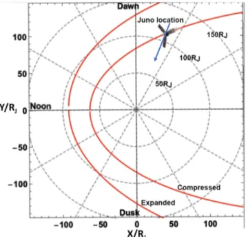
Figure 1 shows the locations of the magnetopause from the Joy et al. (2002) model when the magnetosphere is expanded (the outer red curve) and compressed (the inner red curve). It also shows that Juno's location during the XMM-Newton observation was consistent with the spacecraft being in the outer magnetosphere and close to the magnetopause if the magnetosphere was compressed.
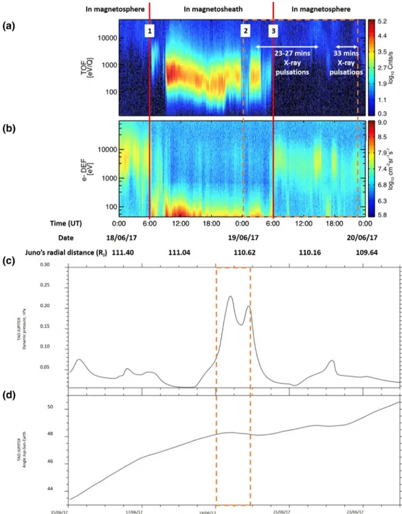
Data from the JADE instrument onboard Juno (Figures 2a and 2b) reveal that the spacecraft moved from Jupiter's magnetosphere to the magnetosheath at least once in the day before XMM-Newton's observation of Jupiter. Juno was inside the magnetosphere before Point 1 on 18 June (day of year 169) at ∼06:00 UT. For around 3 hr after this point, JADE detected heated solar wind ions with energies ∼100–1,000 eV/q (panel a) and high-energy electrons (panel b) from the magnetosphere. This would mean that the space-craft was in a boundary layer before entering the magnetosheath as indicated by the high count rates of solar wind ions and low-energy (<100 eV) electrons. There seems to be another magnetopause crossing when XMM-Newton's observation of Jupiter started at around 00:00 UT on 19 June (day of year 170) (Point 2) as shown by the decrease in the count rate of high-energy ions. However, there are still detections of low-energy electrons that could be from the magnetosheath, and this suggests that Juno was still close to the magnetopause. The spacecraft left this boundary layer and came back inside the magnetosphere at around 06:00 UT (Point 3) later on that day, hinting that the magnetosphere was slightly less compressed from this moment. However, it is difficult to determine how quickly the magnetosphere was expanding by after this point. There are also hints of low-energy electrons and ions with energies of ∼1,000 eV/q at ∼09:00 UT and ∼17:00 UT on 19 June, which could have been brought into the magnetosphere from the magnetosheath by Kelvin-Helmholtz instabilities. Juno had only moved ∼1 RJbetween Points 1 and 3, and this distance is too small to be shown in Figure 1. This figure also marks the moments in time where the X-ray pulsations were detected by XMM-Newton.
Figure 1. Juno's location during the XMM-Newton observation in June 2017. The spacecraft was in the dawn flank of
Jupiter's magnetosphere at 4.3–4.5 LT and had a distance of∼110 RJfrom the planet. The red curves mark the magnetopause locations for Jupiter's expanded (outer contour) and compressed (inner contour) magnetospheres with standoff distances of 92 RJand 63 RJrespectively as predicted by the Joy model (Joy et al., 2002). The dashed concentric circles indicate distances from Jupiter (at the center) in steps of 50 RJ. Juno was situated where the magnetopause is expected to be for a nose standoff distance of 62.52 RJas reported in Weigt et al. (2020). The blue arrow indicates Juno's trajectory.
Before Juno's arrival at Jupiter, solar wind propagation models were used to estimate the parameters of the solar wind at Jupiter (e.g., Dunn et al., 2016; Kimura et al., 2016) to complement observations of the X-ray auroras. Here, we compare the in situ data from Juno with a model that simulates a one-dimensional MHD propagation of the solar wind at Jupiter (Tao et al., 2005) (Figures 2c and 2d). Panel (c) displays the solar wind dynamic pressure upstream of Jupiter and shows that it is greatest during the time of the XMM-Newton observation, further supporting the claim that the magnetosphere was experiencing a compression. This particular model can predict the arrival time of a solar wind compression with a maximum error of ±2 days when the angle between the Earth and Jupiter with respect to the Sun is below 60◦, which is shown in panel (d).
Studies of Jupiter's UV auroras show that they respond greatly to changes in the conditions of Jupiter's mag-netosphere. Grodent et al. (2018) reported that the UV auroras can be divided into six different morphology families and are influenced by both internal conditions (e.g., Io's volcanic activity) and external conditions (e.g., the solar wind) (e.g., Yao et al., 2019). Therefore, the state of the UV auroras can also be used as an indication of how compressed the magnetosphere was.
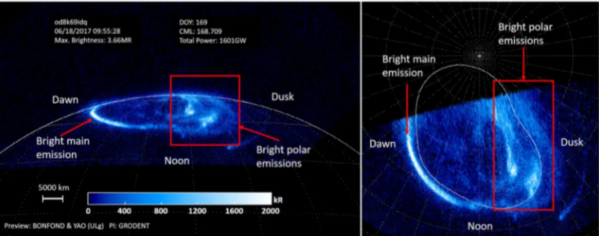
In particular, the “external perturbations” family are very distinct due to the very strong main emission in the dawn sector that also features a very bright and narrow arc. This arc is separated from the discontinuity at ∼10:00 LT by a sharp boundary. Furthermore, the main emission in the afternoon sector is similarly bright and narrow. The duskside often displays bright polar emissions and arcs poleward of and parallel to the main emission that are bright and pulse strongly. The authors conclude that auroras from this family arise when the magnetosphere is compressed by increased interplanetary medium activity. Figure 3 is a snapshot of the UV aurora as viewed by the Hubble Space Telescope 14 hr before the start of XMM-Newton's observation. The thickness and brightness of the main oval and bright polar emission in the image are consistent with the morphology associated with this family. This type of morphology was also reported during solar wind compressions in Nichols et al. (2009, 2017). For images and summaries of the other family groups, see Figure S1 and Text S2.
Journal of Geophysical Research: Space Physics
10.1029/2019JA027676
Figure 2. Ion time of flight (TOF) (panel a) and electron differential energy flux (DEF) (panel b) data from Juno's
JADE instrument. The dashed orange box marks the duration of XMM-Newton's observation of Jupiter. The white horizontal lines show the intervals when the X-ray auroras were pulsating with different periods. Panel (c) shows the propagation model of the solar wind dynamic pressure (Tao et al., 2005) at Jupiter's magnetopause in the days before and after the observation. Panel (d) shows the angle between the Earth and Jupiter with respect to the Sun during the same period. The orange box corresponds to XMM-Newton's observation.
Figure 3. The northern UV aurora as observed by the Hubble Space Telescope (HST) 14 hr before XMM-Newton's
observation. The left panel shows the aurora as it is seen by the HST, and the right panel is of a polar projection of the same HST observation. Grodent et al. (2018) define six families of aurora morphology. The morphology exhibited here represents a modest case of externally driven (i.e., by the solar wind) auroral morphology. One factor indicative of this is the thick and bright main emission in the dawn sector, which is triggered by the compression (Nichols et al., 2009, 2017; Yao et al., 2019). The color scale shows the brightness of the aurora with white being areas with the brightest UV emissions.
3. Temporal Analyses
Jupiter's X-ray auroras have been reported to pulse regularly with periods of tens of minutes (Dunn et al., 2016, 2017; Gladstone et al., 2002; Jackman et al., 2018). However, Branduardi-Raymont et al. (2007) and Elsner et al. (2005) found no evidence of strictly regular periodicities in the three observations made in 2003. These pulsations are not unique to the X-ray auroras as the northern UV aurora has also been found to flare periodically every 2–3 min and map to regions with closed magnetic field lines (Bonfond et al., 2011, 2016). Watanabe et al. (2018) also report periodicities of tens of minutes in the IR aurora.
The data were first reduced, cleaned, and calibrated by the XMM-Newton Pipeline Processing System (PPS) (for more details, see the XMM-Newton Users Handbook, Issue 2.17, 2019). Jupiter is a moving target, so in order to produce an image of the entire planet, each X-ray photon was reregistered onto Jupiter's disk. The XMM-Newton Science Analysis Software (SAS) is a collection of tasks, scripts, and libraries that was subsequently used to analyze the data obtained in this observation by XMM-Newton. SAS Version 17.0.0, released on 21 June 2018, was used in this study. An image of Jupiter was first produced using a Graphical User Interface (GUI) metatask called xmmselect (see Figure S2). The auroral and equatorial regions were then isolated in the SAOImage DS9 astronomical imaging and data visualization application. Light curves and spectra of those regions were then extracted by xmmselect.
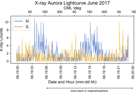
Jupiter's X-ray auroras are fixed on the planet's frame and are located between 155–190◦and 0–75◦Central Meridian Longitude (CML) for the northern and southern auroras respectively when using the left-handed System 3 coordinate system. The light travel time-shifted light curve of XMM-Newton's June 2017 observa-tion demonstrates Jupiter's ∼10-hr rotaobserva-tion period as the auroras come in and out of view (Figure 4) and is more easily seen for the northern aurora (in blue). Therefore, it was necessary to analyze only the sections of the light curve that correspond to the times when the auroras are visible in order to determine whether there are any quasiperiodic pulsations. The auroras are visible when the CMLs are between 65–280◦and 270–165◦for the north and south, respectively (±90◦from the auroral CMLs) (e.g., Dunn et al., 2017), and this is also shown in Figure 4. The NASA JPL HORIZONS Web-Interface was used to create an ephemeris to determine the times when the CMLs were between the desired figures resulting in two viewing periods for the north and three for the south. The binning for this light curve is 180 s and incorporates data from the EPIC-pn, EPIC-MOS1, and EPIC-MOS2 cameras.
The northern aurora is usually observed to be comparatively brighter than its southern counterpart, and it is proposed to be so because of a more favorable viewing geometry. However, it could also be due to different local conditions at the poles, such as the magnetic field being stronger at the north. The southern aurora appears to release two very bright flares near the end of the observation, at 21:00 UT and 22:00 UT on 19
Journal of Geophysical Research: Space Physics
10.1029/2019JA027676
Figure 4. XMM-Newton EPIC (coadded pn, MOS1, and MOS2) 3-min binned light curves of the X-ray auroras. It has
been shifted to account for Jupiter being∼42 light minutes away from the Earth at the time of the observation.
June (see Figure 4). These flares emitted a high flux of photons that is usually only seen coming from the north. Figure S3 shows error bars associated with the count rates and the CML ranges of when the auroras are visible.
3.1. Wavelet Transform
We applied discrete wavelet transforms over the entire observation to reveal if, when, and for how long the auroras pulsate. The data were first grouped into 120-s bins. The time and period resolution of the power spectral density (PSD) produced by this method is low; therefore, an exact time of occurrence and precise period of the pulsations cannot be determined. However, the PSD provides a visual representation of these pulsations and gives estimates of which time intervals to investigate further using a method that does not provide simultaneous time and period resolution, such as a fast Fourier transform (FFT). Several differ-ent types of wavelets, including Gaussian, complex Gaussian, Morlet, complex Morlet, frequency B-spline, Mexican hat, and Shannon, were tried to see which best represents the behavior found in the light curve. We found that the Shannon wavelet best replicated the known periodicities in the Jovian X-ray light curves because the resulting PSD clearly distinguishes each planetary rotation and seems to minimize the effects of noise at longer periods. Shannon wavelets also provide good period resolution, which is what was required for this study.
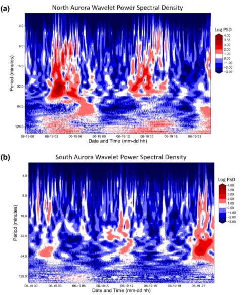
Figure 5 shows the PSD plots from the wavelet transforms using a Shannon wavelet. The PSD plots for the other wavelets are shown in Figures S4 and S5. Areas in dark red are periods where the light curve exhibits strong pulsations and the significance of the pulsations decreases as the red becomes lighter. Areas in blue have no regular periodicities in the light curve. We can determine the intervals where the auroras are visi-ble by looking for regions in red. The finger-like structures that appear to show pulsations with periods of ∼4–16 min are a result of the PSD analysis. Each time bin only has a discrete low number of X-ray photon counts; therefore, different time bins produce fingers of different widths. A true quasiperiodic pulsation sig-nal on these PSDs would be a red region that has a width larger than the finger-like structures. Figure S6 displays the Shannon PSD plots of the northern aurora with different time bins. Notice the finger-like structure increasing with larger time bins.
The first viewing of the northern aurora (panel a) has a very strong pulsation period of ∼20–40 min at just after 03:00 UT, which persisted until around 06:00 UT at a lower power as shown by the lighter red region. The PSD here traces a red curve that also hints that the period lengthens in a smooth fashion within this time interval. However, the significance is low and is hard to establish within the wavelet transform. A similar period also exists during the second rotation; however, its power is not as great. This behavior does not last for the entire rotation but stops at around 15:30 UT. The southern aurora (panel b) shows some moderate
Figure 5. Discrete Shannon wavelet transforms of the X-ray auroras light curves (2-min time resolution). Panel (a) is
for the northern aurora, and panel (b) is for the southern aurora. The color bar shows power spectral density (PSD) on a log scale from 2−3to 24. See text for details.
continuous 20- to 30-min pulsations between 09:00 and 12:00 UT and then bright 45-min pulsations through the third observing window from 20:00 UT until the end of the observation (the bright flares in Figure 4). All of these features are also found in the PSDs for the different wavelets in Figures S4 and S5. Vertical cuts of the PSD plots are also shown in Figures S7 and S8.
3.2. Fast Fourier Transform
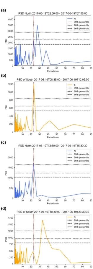
The wavelet transforms of the entire ∼23-hr-long light curve identified four pulsating intervals that required further analysis with FFT in order to gain higher-resolution insights into any periodic behavior. The four intervals were taken to be between 02:56–07:56 UT (first rotation in the north), 08:35–12:05 UT (second rotation in the south), 12:50–15:30 UT (second rotation in the north), and 18:30–23:39 UT (third rotation in the south). The first rotation in the south was confirmed to not have any significant regular pulsations as shown in Figure S9. To increase the temporal resolution, the light curve was first rebinned so that each bin lasts for 30 s. The peaks in the resulting PSD reveal the periods of any existing quasiperiodic behaviors. Figure 6 shows the PSDs of the rotations that had significant pulsations, namely, Rotation 1 for the north (PSD A), part of Rotation 2 for the north (PSD C), and Rotations 2 (PSD B) and 3 (PSD D) for the south. To test the statistical significance of these intervals, we generated 10,000 simulated light curves using Monte Carlo methods with the same number of photons as the given window. From this, we determined how often a periodicity of the observed power would be randomly generated. We show the 99th, 90th, and 66th
Journal of Geophysical Research: Space Physics
10.1029/2019JA027676
Figure 6. Fast Fourier transform PSD in the order (from the top) that each aurora viewing occurred. Panels (a) and (c)
are for the complete first and part of the second rotations of the northern aurora, respectively. Panels (b) and (d) are for the first half of the second and complete third rotations of the southern aurora. The 66th, 90th, and 99th percentiles are marked by the dashed, dashed dot, and dotted black lines, respectively. The vertical red dashed line marks the recurring period at∼23 min.
percentiles from these methods on the plots. Below, we discuss each auroral viewing in the time order it occurred.
There was no statistically significant quasiperiodic behavior in XMM-Newton's light curve during the first viewing period of the southern aurora, which is consistent with the findings from the Chandra data set (Weigt et al., 2020).
PSD A in Figure 6 is for the first viewing period of the northern aurora. The largest peak occurs at ∼27 min, indicating that this is the period of the strongest pulsation. In addition, independent analysis of Chan-dra's light curve that partially overlaps with XMM-Newton's also shows pulsations in the north. ChanChan-dra's observation (that commenced around 5 hr before XMM-Newton started observing) also showed a 26-min period (Weigt et al., 2020) in the X-ray aurora, implying that this periodic oscillation was observed by both instruments independently. There is another smaller peak at ∼23 min that reaches up to the 90th percentile. The southern aurora comes back into XMM-Newton's view at 08:35 UT. It was difficult to determine from Figure 5 whether there were any significant quasiperiodic oscillations within this rotation. The FFT reveals that there is a strong pulsation at ∼23 min during the first half of this rotation (PSD B). This may suggest that there is a global mechanism that allows Jupiter's northern and southern X-ray auroras to sometimes pulsate with the same period. Alternatively, it may show that both the northern and southern auroras were connected to an LT sector with this characteristic oscillation at respective times during the observation. The wavelet transform (Figure 5) continues to show periodic pulsing when the northern aurora rotates back into view at 12:50 UT, which lasts until 15:30 UT. PSD C shows that there is continued pulsing at a ∼23-min period that is also at the 99th-percentile level. We note that this suggests that Jupiter exhibited a sustained 23-to 27-min pulsation for at least two Jupiter rotations (and possibly a third including the Chandra observation prior to this (Weigt et al., 2020).
PSD D corresponds to the section of the light curve that exhibits the bright southern flares. The strong peak at ∼33 min reflects the regularity of the series of prominent southern flares occurring at the end of the observation.
4. Spectral Analyses With XSPEC
Spectra were extracted from the EPIC-pn camera data during the periods when the auroras were visible resulting in two spectra for the north and three for the south. They were binned to have at least 10 counts in each channel for the𝜒2fit statistics to be applicable while maintaining the highest possible spectral resolution. Each spectrum was fitted with the X-ray spectral fitting tool XSPEC (v. 12.10.0c released on 8 October 2018) using the Atomic Charge Exchange (ACX) package (Smith et al., 2012) that models spectra from an astrophysical plasma undergoing charge exchange.
The ACX package comprises two models based on charge exchange processes and the DACX program. The standard ACX model allows the plasma to keep colliding until it is neutralized. Within this model, the Solar Wind Charge Exchange (SWCX) flag can be switched on or off. If it is switched on, then only one collision between each ion and neutral is permitted, and this results in fewer emission lines for a particular temper-ature and normalization value when compared to the standard model. The SWCX flag was switched off for this study, and the standard model was used to fit the spectra. Switching the SWCX flag on does not change the fit; however, it does result in slightly different oxygen-to-sulfur ratios (see Dunn, Branduardi-Raymont, et al., 2020; Dunn, Gray, et al., 2020 for more details).
ACX also allows the user to set the initial ion abundances and freeze the abundance of any particular ion. XSPEC produces a count spectrum that predicts what the spectrometer in a particular channel should detect for the chosen ion abundances and ion temperature and compares this count spectrum with the observed spectrum so that a fit statistic is calculated. The process is repeated with different parameter values until the best fit statistic and therefore the best fit ACX model is found. The second model is named acxion, which is primarily used to display the spectral shape of charge exchange emissions for particular ions (Smith & Foster, 2014).
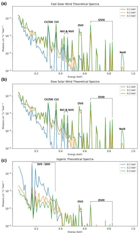
We wanted to test whether solar wind or iogenic plasma better fit the Jovian auroral spectra and also what difference different solar wind ion populations would make. We created three comprehensive models in ACX to do this. The first and second models comprised the actual ion abundances from the fast and slow
Journal of Geophysical Research: Space Physics
10.1029/2019JA027676
Figure 7. Theoretical X-ray emission spectra for the fast solar wind (panel a), slow solar wind (panel b), and iogenic
ion populations (panel c) at three given ion temperatures of 0.1, 0.2, and 0.3 keV.
solar wind as measured by the Solar Wind Ion Composition Spectrometer on the Ulysses spacecraft, respec-tively (von Steiger et al., 2000). The third was iogenic in nature and only consisted of sulfur and oxygen ions. Figure 7 shows the resulting theoretical X-ray spectra that would be produced by these models. The oxygen-to-sulfur ratio used to produce the iogenic theoretical spectra was 0.41 as this is the average ratio measured by the JADE instrument on Juno (Kim et al., 2019).
Table 1
Ion Abundances Relative to the Solar Photosphere Abundances (von Steiger et al., 2000) Used in Each Model
C N O Ne Mg Si S Fe
Fast solar wind 1.62 0.86 1.00 0.57 2.38 2.60 2.88 1.57
Slow solar wind 1.57 0.69 1.00 0.67 3.24 3.59 2.69 2.06
Iogenic 0 0 0.07–0.33 0 0 0 9.52–10.91 0
Note.The fast and slow solar wind abundances were kept fixed in the fits. The sulfur and oxygen abundances for the iogenic model are the minimum and maximum best fit values over all rotations for the north and south auroras.
The ion abundances for the solar wind models were kept fixed at the values in Table 1, and the only parame-ters that were left free in the fits were the ACX (ion) temperature and ACX normalization. A bremsstrahlung emission was also included in the model to represent the underlying continuum extending to higher ener-gies than the charge exchange emission. The bremsstrahlung temperature and normalization were left free in the fits. The four fitted parameters were also left free when fitting with the iogenic model; however, the sulfur and oxygen abundances were free too this time, so that the oxygen-to-sulfur ratio, which is known to change with space and time, was allowed to vary. The abundances for the other ions were fixed at zero. Notice in Table 1 that the iogenic model only requires a small fraction of oxygen ions relative to the solar photosphere and roughly 10 times more sulfur than what is found in the solar wind to give good fits. This gives oxygen-to-sulfur ratios that closely match the ratios observed in Jupiter's magnetosphere. The theoret-ical emission spectra for the fast and slow solar wind appear to be almost identtheoret-ical (see Figure 7); however, the spectral fits that they produced had subtle variations and gave different reduced𝜒2values.
4.1. Best Fits for the Auroral Spectra
The best fits for all of the north and south auroral spectra of Jupiter are shown in Figures 8 and 9, respectively. The best fit parameters for the northern aurora are in Table 2 and for the southern aurora in Table 3. The spectral fits of each model for both poles can be found in Figures S10–S14.
The iogenic model gave a much better fit than the solar wind models for the first auroral spectrum from the north as it gave the smallest reduced𝜒2value of 1.11 for 28 degrees of freedom. All three models gave very similar reduced𝜒2values for the second northern aurora spectrum with 0.98 for the iogenic model, 0.99 for the slow solar wind model, and 1.01 for the fast solar wind model. The ACX temperature is defined as the temperature of a thermal plasma. However, the aurora producing plasma is not thermal. Therefore, we use the ACX temperature as an approximation of the energy state of the plasma. Increases in this temperature represent a more energetic precipitating ion population and therefore a higher charge state distribution. The two rotations of the northern aurora required very similar ion temperatures, and the contribution of the ACX model to the entire fit is determined by its normalization, which remained consistent throughout the observation.
Both northern auroral spectra also required a bremsstrahlung continuum to get good fits. A bremsstrahlung temperature higher than 100 keV is an unrealistic temperature since it is much higher than the operational range of EPIC, but it is used to represent the underlying continuum. Its contribution does not vary between the two rotations. The northern main UV auroral oval in Figure 3 appeared very bright 14 hr before the start of this XMM-Newton data set. This type of morphology is expected to remain bright for multiple Jupiter rota-tions and may explain why the bremsstrahlung model contributed to the fits as much as the ACX model given that both bremsstrahlung and UV emissions are expected to be produced by the same electron population. In situ measurements of Jupiter's magnetosphere by Juno's JADE instrument reveal that the oxygen-to-sulfur ratio varies between 0.2 and 0.6 with a mean value of 0.41 ± 0.09 (Kim et al., 2019). The values obtained by our X-ray fits are above what JADE reported, although they are still (except for the first northern and third southern rotations) within the values of 0.83-20.00 (or sulfur-to-oxygen ratios of 1.20-0.05) that are quoted in Radioti et al. (2006) and close to that of 1.02 from the physical chemistry model (Delamere et al., 2005). Using the ratios 0.83 and 1.02 gave very similar results to the best fit. A ratio of 0.83 gave reduced𝜒2values between 0.97 and 2.11 for both poles, while a ratio of 1.02 gave reduced𝜒2values between 0.94 and 2.27. The largest ratio of 20.00 gave much poorer fits with reduced𝜒2values between 1.64 and 3.78.
Journal of Geophysical Research: Space Physics
10.1029/2019JA027676
Figure 8. The best fits for the northern aurora in panels (a1) and (b1) are represented by the histograms and the data
points by the crosses. The theoretical models are shown in panels (a2) and (b2). The solid and dashed lines in these two panels display the dominant and recessive model respectively at any given energy.
Fitting the spectra with XSPEC also gives the flux of the auroras based on the chosen models. Table 2 shows that the luminosity of the northern soft and hard X-ray auroras remained relatively steady throughout the observation.
The fits for the first spectrum of the southern aurora gave slightly conflicting results as the slow solar wind model actually returned a smaller reduced𝜒2value of 1.24 for 15 degrees of freedom compared to 1.30 for 13 degrees of freedom from the iogenic model. However, the iogenic model fits the spectrum much better visually (see Figure S15), and this is why this model was chosen as the best fit. The difference in the reduced 𝜒2value between the two models is purely due to the slow solar wind model having more parameters frozen as when the sulfur and oxygen abundances for the iogenic model were also frozen, the𝜒2value for this model falls below that of the slow solar wind (1.12 vs. 1.24 for 15 degrees of freedom). All three models for the third southern aurora spectrum gave reduced𝜒2values larger than 2 as a result of the spectrum not having any strong emission lines (Spectrum C in Figure 9).
Figure 9. The best fits for the southern aurora in panels (a1), (b1), and (c1) are represented by the histograms and the
data points by the crosses. The theoretical models are shown in panels (a2), (b2), and (c2). The solid and dashed lines in these three panels display the dominant and recessive model respectively at any given energy.
Journal of Geophysical Research: Space Physics
10.1029/2019JA027676
Table 2
Best Fit Spectral Parameters for the Northern Aurora
First rotation Second rotation
Best fit model Iogenic Iogenic
Reduced𝜒2 1.11 0.98
Degrees of freedom 28 40
ACX temperature (keV) 0.20±0.01 0.17±0.01
ACX normalization (1.25±0.14)×10−6 (1.51±0.15)×10−6
O-to-S ratio 0.74±0.19 0.99±0.24
Bremsstrahlung temperature (keV) 180±86 300±88
Bremsstrahlung normalization (5.91±1.16)×10−6 (7.76±1.07)×10−6 Luminosity of soft (0.2–2.0 keV) X-rays (GW) 0.37±0.05 0.32±0.03 Luminosity of hard (2.0–10.0 keV) X-rays (GW) 0.13±0.05 0.15±0.01
The first and second southern auroral spectra had comparable ACX temperatures with each other and with the northern aurora; however, the third spectrum needed a much higher temperature. The ACX nor-malization for the third rotation is much lower than in the previous two, which may suggest that the contribution from charge exchange decreased for this rotation. However, the soft X-ray luminosity did not change throughout the observation. We also note that the ACX temperature and normalization are not independent of each other.
We also combined the iogenic and bremsstrahlung models with the two solar wind models by freezing all of the best fit parameters other than the normalizations of each model. This allows us to confirm which one is the dominant model. The results are in Tables 4 and 5. The iogenic model has a normalization that is at least one order of magnitude larger than the solar wind models, which further supports the argument that the majority of the precipitating ions are from inside the magnetosphere and any contribution from the solar wind is very small. The normalizations of the solar wind models reduced to effectively zero for the second and third south rotations, which means that all of the precipitating ions were originally from Io's volcanoes during these rotations. Furthermore, the bremsstrahlung model has comparative normalizations to the iogenic model, which shows that it is necessary in order to get good fits. The reduced𝜒2for when each type of solar wind model is combined with the iogenic model are identical due to the two solar wind models being very similar to each other. The spectra for each of these fits can be found in Figures S16–S20.
5. Discussion
The Jupiter data set obtained by XMM-Newton in June 2017 is unique as it is the first to occur during a solar wind compression event confirmed by Juno's in situ measurements of the conditions in the region near to the magnetopause (Figures 1 and 2). The light curves and spectra taken with XMM-Newton's EPIC-pn,
Table 3
Best Fit Spectral Parameters for the Southern Aurora
First rotation Second rotation Third rotation
Best fit model Iogenic Iogenic Iogenic
Reduced𝜒2 1.30 1.38 2.12
Degrees of freedom 13 10 12
ACX temperature (keV) 0.17±0.01 0.14±0.01 0.63+0.24−0.33
ACX normalization (1.02±0.18)×10−6 (1.44±0.28)×10−6 (3.65±0.59)×10−7
O-to-S ratio 0.88±0.40 1.59±0.95 0.34±0.19
Bremsstrahlung temperature (keV) 200±82 193±92 176±92
Bremsstrahlung normalization (5.86±1.16)×10−6 (5.13±1.12)×10−6 (5.09±1.48)×10−6 Luminosity of soft (0.2–2.0 keV) X-rays (GW) 0.21±0.05 0.20±0.05 0.20±0.06 Luminosity of hard (2.0–10.0 keV) X-rays (GW) 0.12±0.04 0.17±0.02 0.15±0.05
Table 4
Normalizations and Reduced𝜒2Values of the FSW, SSW, Io′
, and Bremsstrahlung Models When Combined Together to Fit the Northern Aurora
1st rot FSW + Io′ 1st rot SSW + Io′ 2nd rot FSW + Io′ 2nd rot SSW + Io′ Solar wind normalization (1.69+2.14−1.69)×10−8 (2.03+2.28−2.03)×10−8 (7.43±1.76)×10−8 (8.26±1.85)×10−8 Iogenic normalization (1.15±0.14)×10−6 (1.14±0.14)×10−6 (8.94±1.50)×10−7 (8.55±1.50)×10−7 Bremsstrahlung normalization (5.93±1.14)×10−6 (5.93±1.14)×10−6 (7.63±1.07)×10−6 (7.62±1.07)×10−6
Reduced𝜒2 1.00 1.00 0.86 0.86
Degrees of freedom 31 31 43 43
Abbreviations: FSW = fast solar wind; Io = iogenic; SSW = slow solar wind.
EPIC-MOS1, and EPIC-MOS2 cameras were analyzed to reveal the temporal and spectral characteristics of Jupiter's X-ray auroras.
Figure 4 shows the light travel time-shifted light curve of the X-ray emissions of the entire observation and shows that the auroras from each pole rotate in and out of view. The resulting PSDs (Figure 5) from the wavelet transform method also display this. What is more, these PSDs highlight the time periods when the auroras were pulsating, and a more thorough analysis of this behavior was then applied to the data. Running FFTs on those specified intervals (Figure 6) demonstrate that the northern aurora pulsates every 23–27 min over an interval of ∼12.5 hr, suggesting that the aurora and its magnetospheric driver may have maintained a regular oscillation for more than one Jupiter rotation. Concurrent observations from Chandra also found periodicities of 26–37 min in the X-ray aurora (Weigt et al., 2020). These periodicities have been reported before, and they also occurred during a solar wind compression (Dunn et al., 2016). The southern aurora did not show any quasiperiodic behavior at the start of the observation; however, periods of 23 and 33 min developed over the two subsequent rotations, respectively. While Dunn et al. (2017) highlight intervals when the auroras can behave independently, the shared periodicity in our observation suggests that there are also intervals when both the northern and southern auroras share a driver that oscillates with this frequency. It may be the case that there is an LT sector that is characterized by this oscillation, and when each aurora maps to this, then they exhibit the oscillation. Alternatively, one pole could start pulsing that sets up a charge imbalance that forces particles to flow out and move along the field lines. These particles would then enter the opposite pole after some time and cause the aurora here to pulse with the same period. Therefore, the second pole would only start to pulse after it has received the incoming particles.
The cause of the pulsations that the X-ray auroras sometimes exhibit is currently unclear. However, a num-ber of mechanisms and explanations have been proposed. The HI-SCALE instrument onboard the Ulysses spacecraft detected periodic changes every 15–20 min and every 40 min in the intensity, anisotropy, and spectral properties of high-energy ions and electrons upstream from Jupiter's bow shock, which may hint at a link between the aurora and the solar wind (Dunn et al., 2016; Marhavials et al., 2001). Moreover, the study by Dunn et al. (2016) also coincided with a solar wind compression event and a pulsation of ∼26 min was also observed then. However, if this periodicity originated in the solar wind, it is unclear how it would be pre-served traveling across Jupiter's bow shock and magnetosheath. Another explanation could involve ultralow frequency (ULF) waves that have been measured to have periods of ∼10 min (Dunn et al., 2016, 2017; Khu-rana & Kivelson, 1989; Manners et al., 2018; Manners & Masters, 2019). The frequencies of ULF waves depend on the length and the mass content of the perturbed field line. Joy et al. (2002) explain that Jupiter has a bimodal magnetopause distance that depends on how compressed the magnetosphere is. Therefore, if Jupiter's magnetosphere during our observation was compressed to the same size and had a similar mass content as in Dunn et al. (2016), then the very similar pulsations of ∼27 and ∼26 min would be expected. This could also hint at the existence of one or a number of characteristic frequencies in the Jovian system that appear if the magnetosphere is compressed to a specific size. The compression event observed by Juno may well be the trigger for the regular periodicity and act to “switch on” the ULF waves. Shortly after the magne-tosphere is seen to become less compressed, the auroral pulsations lengthen from the regular 23-min period observed for over one Jupiter rotation to the 33-min pulsations seen in the south at the end. Those charac-teristic frequencies would then be reflected in the X-ray pulses at the same frequency. However, the 33-min pulsation occurred ∼12 hr after the magnetosphere started expanding, and it is not known how strong the compression was during this time. Alternatively, the cause could be related to Jupiter's outer magnetic field lines being perturbed by pulsed reconnection with the solar wind that leads to the production of
Journal of Geophysical Research: Space Physics
10.1029/2019JA027676
Ta b le 5 N o rmalizations a nd R educed 𝜒 2V alues of the F SW ,SSW ,I o ′ ,a nd Bremsstr a hlung M odels W hen Combined T ogether to F it the S outhern A u ror a 1st rot FSW + Io ′ 1st rot SSW + Io ′ 2nd ro t F SW + Io ′ 2nd ro t SSW + Io ′ 3r d rot FSW + Io ′ 3r d rot SSW + Io ′ Solar w ind n orm (5.31 + 16 .40 − 5. 31 ) × 10 − 9 (8.59 + 17 .70 − 8. 59 )× 10 − 9 4. 87 × 10 − 19 + 1. 16 × 10 − 8 − 4. 87 × 10 − 19 9. 41 × 10 − 20 + 1. 27 × 10 − 8 − 9. 41 × 10 − 20 2. 38 × 10 − 22 + 1. 83 × 10 − 8 − 2. 38 × 10 − 22 3. 13 × 10 − 22 + 2. 07 × 10 − 8 − 3. 12 × 10 − 22 Iogenic n orm (9.63 ± 1.86) × 10 − 7 (9.33 ± 1.86) × 10 − 7 (1.43 ± 2. 80 ) × 10 − 7 (1.43 ± 2.80) × 10 − 7 (2.98 ± 0. 58 ) × 10 − 7 (2.98 ± 0.58) × 10 − 7 Br emsstr a hlung n orm (5.75 ± 1.16) × 10 − 6 (5.75 ± 1.16) × 10 − 6 (5.19 ± 1. 12 ) × 10 − 6 (5.19 ± 1.12) × 10 − 6 (6.92 ± 1. 48 ) × 10 − 6 (6.91 ± 1.48) × 10 − 6 R educed 𝜒 2 1.05 1.05 1.06 1.06 1.70 1.70 Degr ees of fr eedom 16 16 13 13 15 15 Abbr eviations: FSW = fast solar w ind; Io = iogenic; SSW = slow solar wind.arcs or spots of emissions in UV. These pulsed reconnections are estimated to have an interpulsed period of ∼30–50 min (Bunce et al., 2004).
Spectra for the north and south auroras were fitted with charge exchange models involving solar wind and magnetospheric ion populations with the latter giving the best fits for the entire observation period. Each spectrum also needed to include a bremsstrahlung continuum to produce good fits and the bremsstrahlung contribution stayed steady throughout the ∼23 hr. Moreover, the temperatures are all consistent with each other except for the last southern spectrum. The normalizations vary somewhat, but the luminosities appear steady.
Three comprehensive models of the fast solar wind, slow solar wind, and iogenic ion populations were cre-ated and fitted to the auroral emission spectra to determine the origin of the precipitating ions that produced the soft X-ray emissions during the magnetospheric compression event. The iogenic model gave best fits for the auroral emissions at the poles throughout the observation, and this is consistent with the findings of Dunn et al. (2016) and Elsner et al. (2005) and with the theory from Cravens et al. (1995) and Bunce et al. (2004). Combining the solar wind and iogenic models also showed that the iogenic model was more dominant and that the majority of the precipitating ions are from inside the magnetosphere.
The morphological results from Weigt et al. (2020) suggest that the X-ray hot spot is elongated and could possibly explain why Dunn et al. (2016) witnessed two separate sources for the X-ray auroras. The first source may be from precipitating magnetospheric sulfur ions that originate from a region of closed field lines at 50 to 70 RJ. The second source may be from open-field lines that map closer to the magnetopause, and the ion population seem to be a mixture of oxygen and sulfur or carbon. This may explain why the iogenic model gives the better fits in this study.
6. Conclusion
Results of the analysis of XMM-Newton's observation of Jupiter on 19 June 2017, for the first time coinciding with a well-established magnetospheric compression event, are presented. Wavelet and FFTs reveal that shortly after this magnetospheric compression, the X-ray auroras are observed to pulse with a recurring periodicity of 23–27 min, which lasts more than 12.5 hr (longer than one Jupiter rotation) and is seen to be exhibited by both the northern and southern auroras. The southern aurora continues to flare very brightly, and its pulsation period lengthens to 33 min.
Analyzing the auroral spectra using the ACX package allowed us to create three comprehensive models to fit the spectra with. Two of those models incorporated the ion abundances measured in the fast and slow solar wind by Ulysses, whereas the third model only contained sulfur and oxygen ions to represent the material in the Io plasma torus. The iogenic model gave best fits throughout the observation, indicating that the precipitating ions responsible for Jupiter's X-ray auroras are, at least during this XMM-Newton observation, originating from the iogenic population.
References
Bhardwaj, A., Branduardi-Raymont, G., Elsner, R. F., Gladstone, G. R., Ramsay, G., Rodriguez, P., et al. (2005). Solar control on Jupiter's equatorial X-ray emissions: 26–29 November 2003 XMM-Newton observation. Geophysical Research Letters, 32, L03S08. https://doi.org/ 10.1029/2004GL021497
Bhardwaj, A., Elsner, R. F., Gladstone, G. R., Waite, J. H., Branduardi-Raymont, G., Cravens, T. E., & Ford, P. G. (2006). Low-to middle-latitude X-ray emission from Jupiter. Journal of Geophysical Research, 111, A11225. https://doi.org/10.1029/2006JA011792 Bonfond, B., Grodent, D., Badman, S. V., Gérard, J.-C., & Radioti, A. (2016). Dynamics of the flares in the active polar region of Jupiter.
Geophysical Research Letters, 43, 11,963–11,970. https://doi.org/10.1002/2016GL071757
Bonfond, B., Vogt, M. F., Gérard, J.-C., Grodent, D., Radioti, A., & Coumans, V. (2011). Quasi-periodic polar flares at Jupiter: A signature of pulsed dayside reconnections? Geophysical Research Letters, 38, L02104. https://doi.org/10.1029/2010GL045981
Branduardi-Raymont, G., Bhardwaj, A., Elsner, R. F., Gladstone, G. R., Ramsay, G., Rodriguez, P., et al. (2007). A study of Jupiter's aurorae with XMM-Newton. Astronomy & Astrophysics, 463(2), 761–774.
Branduardi-Raymont, G., Elsner, R. F., Galand, M., Grodent, D., Cravens, T. E., Ford, P., et al. (2008). Spectral morphology of the X-ray emission from Jupiter's aurorae. Journal of Geophysical Research, 113, A02202. https://doi.org/10.1029/2007JA012600
Branduardi-Raymont, G., Elsner, R. F., Gladstone, G. R., Ramsay, G., Rodriguez, P., Soria, R., & Waite Jr., J. H. (2004). First observation of Jupiter by XMM-Newton. Astronomy & Astrophysics, 424, 331–337.
Bunce, E. J., Cowley, W. H., & Yeoman, T. K. (2004). Jovian cusp processes: Implications for the polar aurora. Journal of Geophysical
Research, 109, A09S13. https://doi.org/10.1029/2003JA010280
Cravens, T. E., Howell, E., Waite Jr, J. H., & Gladstone, G. R. (1995). Auroral oxygen precipitation at Jupiter. Journal of Geophysical Research,
100, 17,153–17,161. Acknowledgments
A. D. W. is supported by the Science and Technology Facilities Council (STFC) (Project No. 2062546). A. J. C., G. B.-R., and W. R. D. acknowledge the support from STFC Consolidated Grant ST/S000240/1 to University College London (UCL). W. R. D was also supported by a SAO fellowship to Harvard-Smithsonian Centre for Astrophysics and by European Space Agency (ESA) Contract No. 4000120752/17/NL/MH. D. M. W. is supported by STFC (Project No. 2115044). C. M. J.'s work at Southampton is supported by STFC Ernest Rutherford Fellowship ST/L004399/1. C. M. J.'s work at DIAS is supported by Science Foundation Ireland Grant 18/FRL/6199. Z. H. Y. acknowledges the Strategic Priority Research Program of Chinese Academy of Sciences (Grant XDA17010201). C. T. acknowledges support from the Japan Society for the Promotion of Science (JSPS) KAKENHI Grant 19H01948. F. A.'s work was funded by the National Aeronautics and Space Administration (NASA) New Frontiers Program for Juno. D. G. acknowledges the financial support from the Belgian Federal Science Policy Office (BELSPO) via the PRODEX Programme of ESA. The Juno JADE data can be obtained from the NASA Planetary Data System (https:// pds-ppi.igpp.ucla.edu/mission/JUNO). The Tao solar wind propagation model can be found at the website (http:// amda.cdpp.eu). The UV auroral images are based on observations with the NASA/ESA Hubble Space Telescope (program HST GO-14634), obtained at the Space Telescope Science Institute (STScI), which is operated by AURA for NASA. All data are publicly available at STScI (https://mast.stsci.edu/portal/ Mashup/Clients/Mast/Portal.html). Ephemeris was created from the NASA JPL HORIZONS Web-Interface (https://ssd.jpl.nasa.gov/horizons.cgi). The raw and calibrated XMM-Newton data can be downloaded from the XMM-Newton Science Archive (http://nxsa.esac.esa.int/nxsa-web/ $\delimiter"005C317$#home). We used the XMM-Newton Science Analysis Software (SAS) (https://www. cosmos.esa.int/web/xmm-newton/ download-and-install-sas), XPSEC (https://heasarc.nasa.gov/docs/ xanadu/xspec/), and Atomic Charge Exchange (ACX) (http://atomdb.org/) to extract and analyze the auroral spectra.
Journal of Geophysical Research: Space Physics
10.1029/2019JA027676
Cravens, T. E., Waite, J. H., Gombosi, T. I., Lugaz, N., Gladstone, G. R., Mauk, B. H., & MacDowall, R. J. (2003). Implications of JovianX-ray emission for magnetosphere-ionosphere coupling. Journal of Geophysical Research, 108(A12), 1465. https://doi.org/10.1029/ 2003JA010050
Delamere, P. A., Bagenal, F., & Steffl, A. (2005). Radial variations in the Io plasma torus during the Cassini era. Journal of Geophysical
Research, 110, A12223. https://doi.org/1029/2005JA011251
den Herder, J. W., Brinkman, A. C., Kahn, S. M., Branduardi-Raymont, G., Thomsen, K., Aarts, H., et al. (2001). The reflection grating spectrometer on board XMM-Newton. Astronomy & Astrophysics, 365(1), L7–L17.
Dunn, W. R., Branduardi-Raymont, G., Carter-Cortez, V., Campbell, A., Elsner, R., Ness, J.-U., et al. (2020). Jupiter's x-rays 2007 Part 1: Jupiter's x-ray emission during solar minimum. Journal of Geophysical Research: Space Physics, 125, e2019JA027219. https://doi.org/10. 1029/2019JA027219
Dunn, W. R., Branduardi-Raymont, G., Elsner, R. F., Vogt, M. F., Lamy, L., Ford, P. G., et al. (2016). The impact of an ICME on the Jovian X-ray aurora. Journal of Geophysical Research: Space Physics, 121, 2274–2307. https://doi.org/10.1002/2015JA021888
Dunn, W. R., Branduardi-Raymont, G., Ray, L. C., Jackman, C. M., Kraft, R. P., Elsner, R. F., et al. (2017). The independent pulsations of Jupiter's northern and southern X-ray auroras. Nature Astronomy, 1, 758–764.
Dunn, W. R., Gray, R., Wibisono, A. D., Lamy, L., Louis, C., Badman, S. V., et al. (2020). Jupiter's x-ray emission 2007 Part 2: Comparisons with UV and radio emissions and in-situ solar wind measurements. Journal of Geophysical Research: Space Physics, 125, e2019JA027222. https://doi.org/10.1029/2019JA027222
Elsner, R. F., Lugaz, N., Waite, J. H., Cravens, T. E., Gladstone, G. R., Ford, P., et al. (2005). Simultaneous Chandra X ray, Hubble Space Telescope ultraviolet, and Ulysses radio observations of Jupiter's aurora. Journal of Geophysical Research, 110, A01207. https://doi.org/ 10.1029/2004JA010717
Gladstone, G. R., Waite, J. H., Grodent, D., Lewis, W. S., Crary, F. J., Elsner, R. F., et al. (2002). A pulsating auroral X-ray hot spot on Jupiter.
Nature, 415(6875), 1000–1003.
Gladstone, G. R., Waite, J. H., & Lewis, W. S. (1998). Secular and local time dependence of Jovian X ray emissions. Journal of Geophysical
Research, 103(E9), 20,083–20,088.
Grodent, D., Bonfond, B., Yao, Z., Gérard, J.-C., Radioti, A., Dumont, M., et al. (2018). Jupiter's Aurora observed with HST during Juno Orbits 3 to 7. Journal of Geophysical Research: Space Physics, 123, 3299–3319. https://doi.org/10.1002/2017JA025046
Houston, S. J., Ozak, N., Young, J., Cravens, T. E., & Schultz, D. R. (2018). Jovian auroral ion precipitation: Field-aligned currents and ultraviolet emissions. Journal of Geophysical Research: Space Physics, 123, 2257–2273. https://doi.org/10.1002/2017JA024872 Jackman, C. M., Knigge, C., Altamirano, D., Gladstone, R., Dunn, W., Elsner, R., et al. (2018). Assessing quasi-periodicities in Jovian X-ray
emissions: Techniques and heritage survey. Journal of Geophysical Research: Space Physics, 123, 9204–9221. https://doi.org/10.1029/ 2018JA025490
Joy, S. P., Kivelson, M. G., Walker, R. J., Khurana, K. K., Russell, C. T., & Ogino, T. (2002). Probabilistic models of the Jovian magnetopause and bow shock locations. Journal of Geophysical Research, 107, SMP 17–1–SMP 17–17.
Kharchenko, V., Bhardwaj, A., Dalgarno, A., Schultz, D. R., & Stancil, P. C. (2008). Modeling spectra of the north and south Jovian X-ray auroras. Journal of Geophysical Research, 113, A08229. https://doi.org/10.1029/2008JA013062
Khurana, K. K., & Kivelson, M. G. (1989). Ultralow frequency MHD waves in Jupiter's middle magnetosphere. Journal of Geophysical
Research, 94(A5), 5241–5254.
Kim, T. K., Ebert, R. W., Valek, P. W., Allegrini, F., McComas, D. J., Bagenal, F., et al. (2019). Method to derive ion properties from Juno JADE including abundance estimates for O+and S2+. Journal of Geophysical Research: Space Physics, 125, e2018JA026169. https://doi. org/10.1029/2018JA026169
Kimura, T., Kraft, R. P., Elsner, R. F., Branduardi-Raymont, G., Gladstone, G. R., Tao, C., et al. (2016). Jupiter's X-ray and EUV auroras monitored by Chandra, XMM-Newton, and Hisaki satellite. Journal of Geophysical Research: Space Physics, 121, 2308–2320. https://doi. org/10.1002/2015JA021893
Manners, H., & Masters, A. (2019). First evidence for multiple-harmonic standing Alfvén waves in Jupiter's equatorial plasma sheet.
Geophysical Research Letters, 46, 9344–9351. https://doi.org/10.1029/2019GL083899
Manners, H., Masters, A., & Yates, J. N. (2018). Standing Alfvén waves in Jupiter's magnetosphere as a source of∼10- to 60-min quasiperiodic pulsations. Journal of Geophysical Research: Space Physics, 45, 8746–8754. https://doi.org/10.1029/2018GL078891 Marhavials, P. K., Anagnostopoulos, G. C., & Sarris, E. T. (2001). Periodic signals in Ulysses' energetic particle events upstream and
downstream from the Jovian bow shock. Planetary and Space Science, 49(10-11), 1031–1047.
Mason, K. O., Breeveld, A., Much, R., Carter, M., Cordova, F. A., Cropper, M. S., et al. (2001). The XMM-Newton optical/UV monitor telescope. Astronomy and Astrophysics, 365(1), L36–L44.
McComas, D. J., Alexander, N., Allegrini, F., Bagenal, F., Beebe, C., Clark, G., et al. (2017). The Jovian Auroral Distributions Experiment (JADE) on the Juno mission to Jupiter. Space Science Reviews, 213(1), 547–643.
McComas, D. J., Bagenal, F., & Ebert, R. W. (2014). Bimodal size of Jupiter's magnetosphere. Journal of Geophysical Research: Space Physics,
119, 1523–1529. https://doi.org/10.1002/2013JA019660
Metzger, A. E., Gilman, D. A., Luthey, J. L., Hurley, K. C., Schnopper, H. W., Seward, F. D., & Sullivan, J. D. (1983). The detection of X rays from Jupiter. Journal of Geophysical Research, 88(A10), 7731–7741.
Nichols, J. D., Badman, S. V., Bagenal, F., Bolton, S. J., Bonfond, B., Bunce, E. J., et al. (2017). Response of Jupiter's auroras to conditions in the interplanetary medium as measured by the Hubble Space Telescope and Juno. Geophysical Research Letters, 44, 7643–7652. https:// doi.org/10.1002/2017GL073029
Nichols, J. D., Clarke, J. T., Gérard, J. C., Grodent, D., & Hansen, K. C. (2009). Variation of different components of Jupiter's auroral emission.
Journal of Geophysical Research, 114, A06210. https://doi.org/10.1029/2009JA014051
Ozak, N., Cravens, T. E., & Schultz, D. R. (2013). Auroral ion precipitation at Jupiter: Predictions for Juno. Geophysical Research Letters,
40, 4144–4148. https://doi.org/10.1002/grl.50812
Ozak, N., Schultz, D. R., Cravens, T. E., Kharchenko, V., & Hui, Y.-W. (2010). Auroral X-ray emission at Jupiter: Depth effects. Journal of
Geophysical Research, 115, A11306. https://doi.org/10.1029/2010JA015635
Radioti, A., Krupp, N., Woch, J., Lagg, A., Glassmeier, K.-H., & Waldrop, L. S. (2006). Correction to “Ion abundance ratios in the Jovian magnetosphere”. Journal of Geophysical Research, 111, A10224. https://doi.org/10.1029/2006JA011990
Smith, R., & Foster, A. (2014). The AtomDB Charge Exchange model.
Smith, R. K., Foster, A. R., & Brickhouse, N. S. (2012). Approximating the X-ray spectrum emitted from astrophysical charge exchange.
Astronomische Nachrichten, 333, 301–304.
Strüder, L., Briel, U., Dennerl, K., Hartmann, R., Kendziorra, E., Meidinger, N., et al. (2001). The European photon imaging camera on XMM-Newton: The pn-CCD camera. Astronomy and Astrophysics, 365(1), L18–L26.
Tao, C., Kataoka, R., Fukunishi, H., Takahashi, Y., & Yokoyama, T. (2005). Magnetic field variations in the Jovian magnetotail induced by solar wind dynamic pressure enhancements. Journal of Geophysical Research, 110, A11208. https://doi.org/10.1029/2004JA010959 Turner, M. J. L., Abbey, A., Arnaud, M., Balasini, M., Barbera, M., Belsole, E., et al. (2001). The European photon imaging camera on
XMM-Newton: The MOS cameras. Astronomy and Astrophysics, 365(1), L27–L35.
Vogt, M. F., Bunce, E. J., Kivelson, M. G., Khurana, K. K., Walker, R. J., Radioti, A., et al. (2015). Magnetosphere-ionosphere mapping at Jupiter: Quantifying the effects of using different internal field models. Journal of Geophysical Research: Space Physics, 120, 2584–2599. https://doi.org/10.1002/2014JA020729
Vogt, M. F., Kivelson, M. G., Khurana, K. K., Walker, R. J., Bonfond, B., Grodent, D., & Radioti, A. (2011). Improved mapping of Jupiter's auroral features to magnetospheric sources. Journal of Geophysical Research, 116, A03220. https://doi.org/10.1029/2010JA016148 von Steiger, R., Schwadron, N. A., Fisk, L. A., Geiss, J., Gloeckler, G., Hefti, S., et al. (2000). Composition of quasi-stationary solar wind
flows from Ulysses/Solar Wind Ion Composition Spectrometer. Journal of Geophysical Research, 105(A12), 27,217–27,238.
Waite, J. H., Bagenal, F., Seward, F., Na, C., Gladstone, G. R., Cravens, T. E., et al. (1994). ROSAT observations of the Jupiter aurora. Journal
of Geophysical Research, 99(A8), 14,799–14,809.
Watanabe, H., Kita, H., Tao, C., Kagitani, M., Sakanoi, T., & Kasaba, Y. (2018). Pulsation characteristics of Jovian Infrared Northern Aurora observed by the Subaru IRCS with Adaptive Optics. Geophysical Research Letters, 45, 11,547–11,554. https://doi.org/10.1029/ 2018GL079411
Weigt, D. M., Jackman, C. M., Dunn, W. R., Gladstone, G. R., Vogt, M. F., Wibisono, A. D., et al. (2020). Chandra observations of Jupiter's X-ray auroral emission during Juno apojove 2017. Journal of Geophysical Research: Planets, 125, e2019JE006262. https://doi.org/10.1029/ 2019JE006262
Yao, Z. H., Grodent, D., Kurth, W. S., Clark, G., Mauk, B. H., Kimura, T., et al. (2019). On the relation between Jovian aurorae and the loading/unloading of the magnetic flux: Simultaneous measurements from Juno, Hubble Space Telescope, and Hisaki. Geophysical
Research Letters, 46, 11,632–11,641. https://doi.org/10.1029/2019GL084201
Erratum
In the originally published version, the manuscript stated that the authors calculated sulfur-to-oxygen ratios, when in fact the values are oxygen-to-sulfur ratios. The text has since been corrected, and this version may be considered the authoritative version of record.