HAL Id: hal-02158565
https://hal-mines-paristech.archives-ouvertes.fr/hal-02158565
Submitted on 18 Jun 2019
HAL is a multi-disciplinary open access
archive for the deposit and dissemination of
sci-entific research documents, whether they are
pub-lished or not. The documents may come from
teaching and research institutions in France or
abroad, or from public or private research centers.
L’archive ouverte pluridisciplinaire HAL, est
destinée au dépôt et à la diffusion de documents
scientifiques de niveau recherche, publiés ou non,
émanant des établissements d’enseignement et de
recherche français ou étrangers, des laboratoires
publics ou privés.
Extended linear formulation of the pump scheduling
problem in water distribution networks
Gratien Bonvin, Sophie Demassey
To cite this version:
Gratien Bonvin, Sophie Demassey. Extended linear formulation of the pump scheduling problem
in water distribution networks. International Network Optimization Conference, June 12-14, 2019,
Avignon, France., pp.13-18, 2019, Open Proceedings, �10.5441/002/inoc.2019.04�. �hal-02158565�
Extended linear formulation of the pump scheduling problem
in water distribution networks
Gratien Bonvin
Center for Applied Mathematics, Mines ParisTech, PSL Research UniversitySophia Antipolis, France [email protected]
Sophie Demassey
Center for Applied Mathematics, Mines ParisTech, PSL Research UniversitySophia Antipolis, France [email protected]
ABSTRACT
This paper presents a generic non-compact linear program-ming approximation of the pump scheduling problem in drinking water distribution networks. Instead of relying on the binary on/off status of the pumps, the model draws on the continuous duration of activation of pump combina-tions, whose entire set is computed in a preprocessing step by ignoring the pressure variation in the water tanks. Pre-processing is accelerated using network partition and sym-metry arguments. A combinatorial Benders decomposition-based local search takes the approximated solution as input to derive a feasible solution. Our experiments on two differ-ent benchmark sets, with fixed- or variable-speed pumps, show the accuracy of the approximated formulation and the ability of the matheuristic to compute near-optimal solutions in seconds, where concurrent, more specialized approaches need minutes or hours.
1
INTRODUCTION
With the evolution of the power sector – because dynamic pricing is a savings opportunity for water network opera-tors [6] – together with advances in mixed-integer nonlinear programming (MINLP), recent years have seen a renewed interest in minimizing the pumping costs in drinking water distribution networks.
The so-called pump scheduling problem is a hard com-binatorial non-convex optimization problem. A variety of solution approaches have been investigated, but they often inefficiently deal with large or medium networks, and many small instances are still open. A first category of approaches (e.g. [6, 7, 10]) combine a numerical simulator, to compute the feasible hydraulic balances, with an exact or heuristic optimization algorithm, to schedule the pump operations at minimum cost. Separating feasibility from optimization makes the convergence of these approaches slow, resulting in sub-optimal solutions. A second category of approaches formulate the whole problem as a MINLP with simplified hydraulic constraints, based either on piecewise-linear ap-proximations (e.g. [8, 9]) or convex relaxations [2, 3, 13]. These approaches only apply to small networks, because of the combinatorial nature of the models, and they may return impracticable solutions. Instead, Burgschweiger et al. [4] keep the non-convex constraints in their model but relax the binary on/off pump activation variables by ag-gregating them. This relaxation is only suitable to large
© 2018 Copyright held by the owner/author(s). Published in Pro-ceedings of the International Network Optimization Conference (INOC), June 12-14, 2019:
Distribution of this paper is permitted under the terms of the Cre-ative Commons license CC-by-nc-nd 4.0.
city-wide networks where dozen of pumps are installed in parallel in each pumping station.
In this paper, we are interested in tackling intermediate-size networks with a mixed approach. We propose to ap-proximate the MINLP model by decoupling feasibility and optimization in the way of Dantzig-Wolfe decomposition: by ignoring the pressure variation in the water tanks, we can compute the feasible hydraulic balances for all pump configurations as a preprocessing step, then derive a non-compact linear programming (LP) model based on the durations of activation of these configurations. We apply network partition and symmetry arguments to acceler-ate the preprocessing without hindering optimality. While the approximated LP solutions may be accurate enough to be practically implemented in pump controllers, we also propose to derive feasible solutions for the original MINLP with a local search approach, adapted from the combinatorial Benders decomposition of Naoum-Sawaya et al. [10]. Finally, we generalize the approach to networks with variable-speed pumps or pressure-reducing valves, which are often overlooked in the literature.
Experiments on the Poormond [6] and Van Zyl [17] benchmark networks show the efficiency of our prepro-cessing, the accuracy of our approximation, and the poten-tial of the overall method to compute near-optimal solutions within seconds where concurrent methods [3, 6, 8, 10, 13] need minutes or hours to compute solutions of higher costs.
The paper is organized as follows: Section 2 defines the problem and describes the standard MINLP formulation in a simplified case. Section 3 presents our non-compact LP formulation and preprocessing reduction techniques and Section 4 the heuristic. Computational results are given in Section 5 and conclusions and perspectives in Section 6.
2
PUMP SCHEDULING PROBLEM
This section describes the problem and a standard formu-lation in the special case, for the sake of simplicity, of a network equipped with unidirectional pipes, fixed-speed pumps and no valves. Comprehensive formulations for more general networks can be found e.g. in [3, 4].
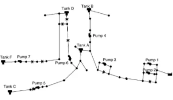
As illustrated in Figure 1, a water distribution network can be represented as a directed graph G = (J, L) with sources JS, junctions JJ and tanks JT as nodes J , and
pipes LP and pumps K as arcs L. Given a time horizon
T of typically one day, the system dynamics are driven by the water demand rate D ∈ RJJ×T
+ at the junctions and
are governed by complex hydraulic laws of conservation of flow and pressure through the network. The problem is to schedule the pump operations over T in order to continuously satisfy the demand and the allowed filling level of the tanks, while minimizing the operation cost.
Figure 1: The Poormond network
A standard model is defined as follows, with x ∈ {0, 1}K×T
the binary on/off state of the pumps, q ∈ RL×T+ the flow
rate through the arcs, and h ∈ RJ ×T+ the head at the nodes
(defined as the sum of pressure and elevation): (P ) : min x,q,h X t∈T X k∈K Ct∆tΓk(xkt, qkt) (1) s.t. X ij∈L qijt= X ji∈L qjit+ Djt, t ∈ T , j ∈ JJ (2) X ij∈L qijt− X ji∈L qjit= σj ∆t (hjt−hjt−1), t ∈ T , j ∈ JT (3) hj0= Hj0, j ∈ JT (4) Hjtmin≤ hjt≤ Hjtmax, t ∈ T , j ∈ J (5) qkt≤ Qmaxk xkt, t ∈ T , k ∈ K (6) hit− hjt= Φij(qijt), t ∈ T , ij ∈ LP (7) (hjt− hit− Ψij(qijt))xijt= 0, t ∈ T , ij ∈ K. (8)
In this model, the time horizon is discretized T = {1, . . . , T } with a resolution ∆t of typically 1 hour in which the
sys-tem is assumed to operate in steady state. Constraints (2) and (3) enforce the conservation of flow at junctions and tanks. In (3), a tank j ∈ JT is assumed to be a vertical
cylinder of area σj which links the stored water volume
linearly to the head. Bounds on heads (4) and (5) depend on the node types: for a tank j ∈ JT, they are given by the
minimum and maximum filling levels, and by the initial level H0
j; for a junction j ∈ JJ, Hjtminstands for the
mini-mum pressure required to serve demand Djt; for a source
j ∈ JS, the head is fixed exogenously. Constraints (7)
en-force the head losses due to friction in pipes. For each directed pipe ij ∈ Lp, the head loss can be accurately
approximated by a quadratic function Φijof the flow.
Con-straints (6) bound the flow through the pumps and bind flow values and pump activation states. Constraints (8) model the head increase through active pumps (if xijt= 1).
For each pump k ∈ K, head-flow coupling function Ψkcan
be accurately fitted from operating points as a quadratic function. Finally, the financial cost is mainly incurred by purchasing electricity for pumping, see objective (1) with Ct≥ 0 the actualized electricity price on period t, and Γk
the power consumption of pump k defined by a linear curve fit Γk(x, q) = λkx + µkq.
Model (P ) is a non-convex MINLP which is often un-tractable even for small networks. One option to solve (P ) is to decrease the resolution of the time discretization, and thus the model size, but it has potential drawbacks: (1) the steady-state assumption is less realistic over longer
time steps, (2) this artificially reduces the set of feasible schedules, and (3) the optimum increases accordingly. We investigate the opposite option, closer to the reality, by allowing to operate pumps at any time.
3
AN APPROXIMATED
NON-COMPACT MODEL
We present a new approximated LP formulation of the pump scheduling problem which separates the computation of the hydraulic balances from the optimization of the schedule. The description is first given in the context of networks where fixed-speed pumps are the only operable elements. We then generalize the definition to networks with valves or variable-speed pumps.
3.1
Tank head approximation
Let A ⊆ L be the set of operable elements of the network, and assume for now that A = K the set of fixed-speed pumps. We call configuration any subset s ⊆ A, also de-noted by its indicator function Is ∈ {0, 1}A defined by
Ias = 1 ⇔ a ∈ s. Configuration s is said active at time
t ∈ T if all its elements, and only these elements, are active (e.g. pumps are on): xat= 1 ⇐⇒ a ∈ s.
Looking at model (P ), a configuration s ⊆ A can be active at time t ∈ T only if, given the tank levels and the allowed variation range, the pumps belonging to the config-uration offer together enough power to increase head and satisfy the demand rate Dtat all junctions. Because water
tanks are usually very large containers, the level variation during 1 hour or less is relatively limited when compared to their heights. We propose to ignore this variation and assume that, at any tank j ∈ JT, the head is fixed to an
ar-bitrary value Hj∗during time step t. Under this assumption,
we can easily compute the hydraulic balance for supplying demand Dt with configuration s. Indeed, by definition, it
is a solution (qt, ht) ∈ RL+ × RJ+ of the non-convex
sys-tem {(2), (5), (6), (7), (8)} restricted to a single time step T = {t} with fixed pump states xat= Ias∀a ∈ A and fixed
tank heads hjt = Hj∗ ∀j ∈ JT. It is known [5, 6, 16] that
this equation system, that we denote Ft(Is, H∗), has at
most one solution which can quickly be computed, in par-ticular, by the Newton method [16] which is implemented in the popular numerical simulator EPANET [11].
To estimate if a configuration s may supply demand rate Dt, we thus propose to check the feasibility of Ft(Is, H∗)
with tank heads arbitrarily fixed to their median values Hj∗ = (Hjmin + Hjmax)/2 for all j ∈ JT. If feasible and
(qs, hs) its solution, we compute the corresponding instan-taneous power consumption Ps
t =
P
k∈s∩KΓk(1, qkts ) and
net fill rate Rsjt =
P ij∈Lq s ijt− P ji∈Lq s
jit at each tank
j ∈ JT. We denote by St∗= {s ⊆ A | Ft(Is, H∗) ̸= ∅} the
set of configurations which may be active during time step t ∈ T according to this assumption.
3.2
Configuration scheduling
Given these estimates, we reformulate the pump scheduling problem as a configuration scheduling problem where, at any time step t, any configuration s ∈ St∗is allowed to be
active for a duration 0 ≤ δst≤ ∆t within the time step.
Modelling the system dynamics boils down to enforce tank head conservation between consecutive time steps, then
leads to the following linear program: (P∗) : min δ,h X t∈T Ct X s∈S∗ t Ptsδst (1’) s.t. X s∈S∗ t δst= ∆t, t ∈ T (9) hjt−hjt−1= X s∈St∗ Rsjt σj δst, t ∈ T , j ∈ JT (3’) Hjtmin≤ hjt≤ Hjtmax, t ∈ T , j ∈ J. (5’)
In (P∗), pumps can thus be operated during time steps. Furthermore, (P∗) is an approximation of (P ), and not just a relaxation: an optimal configuration s at time t for (P ) may not belong to S∗t if it can indeed satisfy demand
Dtbut not under the half-filled tanks assumption; if s does
belong to St∗, otherwise, then its actual consumption may
not be Ps
t precisely.
3.3
Processing configurations
Computing one hydraulic balance with the Newton algo-rithm is almost immediate, but the exponential number of configurations to evaluate, in O(T 2|A|), can make it com-putationally challenging to build (P∗). We propose two techniques to significantly reduce the computation time without hindering optimality.
First, we exploit the symmetries, which are frequent in real data. For instance, when demand rate Dt ∈ RJJ
is constant at all junctions over a number of time steps, then the configurations need to be evaluated on only one time step, since if Dt= Dt′, then S∗t = S∗
t′, Pts= Pts′ and
Rst = Rst′ for all s ∈ S∗t. Another symmetry arises when
pumps with identical characteristics are installed in parallel at a pumping station (see e.g. pumps 1 and 2 in Figure 1). Only one symmetric configuration is then evaluated.
Second, we exploit a partition of the network along the tank nodes. Precisely, we consider the graph G′= (J′, L′) obtained from G by duplicating each tank node j ∈ JT for
each incoming arc ij ∈ L as a new node denoted ji, i.e. J′= J ∪{ji| ij ∈ L, j ∈ JT} and L′= L∪{iji| ij ∈ L, j ∈
JT} \ {ij ∈ L | j ∈ JT}. Once the heads at tanks j ∈ JT
(and at duplicate nodes ji) are fixed to their median values Hj∗, the arc flow and node head values become independent
in each connected component of G′. We thus compute the set of feasible configurations SC
t ⊆ A ∩ LCindependently
for each connected component C = (JC, LC) ∈ CC(G′).
These sub-configurations are then combined by summa-tion: for all s ⊆ A, Ps
t = P C∈CC(G′)Pts∩LC and Rsjt = P C∈CC(G′) | j∈J CR s∩LC
jt for j ∈ JT. Hence, the network
partition reduces both the number of computations and their complexity, being evaluated on smaller graphs. Fur-thermore, the symmetry condition on constant demand occurs with a higher frequency when regarding the subsets of junctions independently.
3.4
Generalization
In most water distribution networks, not only pumps but also valves V ⊆ L of different types can be operated. Like fixed-speed pumps, gate valves and check valves have only two possible states (close or open) and can be modeled in (P ) with a binary variable for each time step (see e.g. [4]).
The definition of configuration can then be extended to A = K ∪ V the set of pumps and valves, saying that a valve is active if it is close. Furthermore, according to [12], Ft(Is, H∗) has still at most one solution.
The presence of variable-speed pumps or pressure-reducing valves deserves more attention as they admit a continuous range of operation modes. A variable-speed pump is either off or operated within an allowed range of speed. For a pressure-reducing valve, the amount of pressure reduction is chosen within a given range and a binary state indicates the direction of the flow (see e.g. [15]). As suggested in [5], we propose to approximate the allowed operation range of each pressure-reducing valve or variable-speed pump a by a discrete set of sample values Aa. The set A is then
augmented with these sample values and a configuration is now defined as s ⊆ A with |s ∩ Aa| ≤ 1. Once pump speeds
and pressure reductions are fixed in configuration s, the Newton method can quickly solve Ft(Is, H∗) as before.
Hence, the approximation model (P∗) and configuration processing scheme apply to a comprehensive class of water networks. Still, the number of configurations to evaluate grows exponentially with the number of operable elements, unless the network partition separates these elements in small sets so that the growth becomes near linear.
4
BENDERS
DECOMPOSITION-BASED HEURISTIC
This section describes an adaptation of the combinatorial Benders decomposition of [10] to search, in the neighbor-hood of the approximated solutions of (P∗), feasible solu-tions to the pump scheduling problem with pump aging constraints.
4.1
Pump aging
While in practice pumps can be operated at any time, too frequent switches are prohibited to prevent premature pump aging. Ghaddar et al. [6] proposed to enforce the following constraints in model (P ) for each pump k ∈ K:
X t∈T ykt≤ N, (10) ykt≥ xkt− xk(t−1), t ∈ T (11) xkt′≥ ykt, t ∈ T , t′∈ [t, t + τ1] (12) zkt≥ xk(t−1)− xkt, t ∈ T (13) xkt′≤ 1 − zkt, t ∈ T , t′∈ [t, t + τ0] (14)
with ykt (resp. zkt) a binary variable equal to 1 if pump
k ∈ K is switched on (resp. off) at time t, N the maximal number of times a pump can be switched on, τ1 (resp. τ0)
the minimum continuous duration a pump is on (resp. off). Naoum-Sawaya et al. [10] designed a combinatorial Ben-ders decomposition approach, where the master integer linear program denoted (M ) is initialized with the ag-ing constraints (10)-(14) alone. At each iteration, (M ) re-turns a candidate schedule X ∈ {0, 1}K×T to evaluate: the EPANET simulator computes the hydraulic balance and power consumption at each time step, sequentially. If a hydraulic constraint is violated or if the partial cost exceeds the best solution known so far at a given time ¯t ∈ T , then the partial schedule up to time ¯t is discarded from the
search by adding a no-good cut to master (M ): ¯ t X t=1 X k∈K Xkt=0 xkt+ X k∈K Xkt=1 (1 − xkt) ≥ 1. (15)
The cut is also added with ¯t = T each time X proves to be the new incumbent, i.e. an improving solution. The algo-rithm stops when (M ) becomes unfeasible. The algoalgo-rithm theoretically converges to a certified optimal schedule, but its slow convergence requires to limit the computation time.
4.2
Truncated Benders decomposition
In the original method [10], the objective function of master (M ) is initialized to 0, then systematically redefined as the minimal distance to the new incumbent, so as to search the next candidate in a neighborhood. Thus, the algorithm improves the solution progressively, as in a local search, but it may start with a low quality solution. We propose to adapt this algorithm to conduct it explicitly as a heuristic to compute good solutions fast. To this end, we initialize the algorithm with an optimal approximate solution δ∗of (P∗), then adjust the distance function, i.e. the neighborhood, iteratively until finding a feasible solution.
More precisely, we first compute the duration δ∗at =
P
s∈S∗ t I
s
aδ∗st of activation of any pump or valve a ∈ A
during time step t ∈ T in the approximated solution. We expect that, in an optimal schedule x, if δ∗at is close to
∆t then a is active during t (i.e. xat = 1), and that, if
δ∗at is close to 0 then a is inactive during t (i.e. xat =
0). Furthermore, we estimate that the daily duration of activationP t∈Txat∆t of a is close to P t∈T δ ∗ at. Hence,
the minimization criterion of (M ) is initialized to: X a∈A X t∈T (∆at− xat∆t)2+ X a∈A (X t∈T ∆at− X t∈T xat∆t)2 (16) with ∆at= ( δ∗at if δ ∗ at∈ {0, ∆t} αat otherwise, and αat∈ {0, δ∗at, ∆t}
is a parameter of diversification which is initialized to δat∗
to search first around the approximated solution of (P∗), and is then updated randomly at each iteration.
Another difference with [10], is that we generalize the method to networks with variable-speed pumps or pressure-reducing valves. In this context, we propose to use a non-convex NLP solver instead of the EPANET simulator to evaluate the candidate solutions X ∈ {0, 1}A×T by solv-ing the slave program, i.e. the standard MINLP formula-tion with the binary variables x fixed to values X. Note here that, unlike for the processing of the configurations (see Section 3.4), we do not extend the definition of the set of operable elements A by discretizing the continuous state range for variable-speed pumps and pressure-reducing valves. Finally, because we run the Benders decomposition as a heuristic, the slave problem is not required to be solved at optimality. Hence, when the global optimization of the restricted non-convex NLP is too time consuming, a fast local optimization solver can be used instead.
5
COMPUTATIONAL RESULTS
We experimented the full heuristic, sketched in Algorithm 1, on two benchmark sets: Poormond [6] and Van Zyl [17]. In this section, we evaluate the solutions in comparison
Algorithm 1: Heuristic for (P )
1 for C ∈ CC(G′), s ⊆ A ∩ LC, t ∈ T do 2 solve F (Is, H∗) with Newton method 3 compute Pts, Rst by summation ∀s ∈ S ∗ t, t ∈ T 4 solve LP (P∗): get δ∗ 5 initialize (M ): min (16) s.t. (10)-(14) 6 while unfeasible do
7 solve MIQP (M ): get X
8 simulate X with Newton method or NLP solver 9 if X feasible then
10 return X
11 else
12 add cut (15) to (M )
13 update (16)
Figure 2: The Van Zyl network
with the best solutions known so far for these instances (see [3] for a comparative analysis of the results published in [3, 6, 10, 13] on Poormond).
5.1
Experimental set-up
The Poormond network, depicted in Figure 1, was derived by [6] from the real water distribution network of Rich-mond, England. It is a medium-size network with 47 nodes including 1 source and 5 tanks, 44 pipes, 7 fixed-speed pumps and 4 gate valves. The benchmark set has five daily instances, denoted from P21 to P25, each corresponding to the real dynamic power tariff, available at [14], that occurred each day in range May 21-25, 2013. The time horizon is discretized in T = 48 time steps of ∆t = 1/2
hour each. Pumps are required to stay on for at least 1 hour (τ1= 2), off for at least 1/2 hour (τ0= 1), and to be
activated at most N = 6 times. The Van Zyl network [17], depicted in Figure 2, is a fictive, small but complex network with 1 source, 2 tanks, 15 pipes, 1 check valve and 3 pumps assumed to be variable-speed pumps after [8]. We experi-mented on this network using the same 5 tariff profiles set at the same time resolution. We denote the five instances Z21 to Z25 accordingly.
The computations were performed on a Xeon E5-2650V4 2.2GHz with 254 GB RAM. The processing of the configu-rations, including the Newton method, was implemented in Python, while the default LP solver and MINLP solver of Gurobi 7.0.2 were run on one thread to solve (P∗) and (M ) respectively. For the Van Zyl instances, the slave problems of the Benders decomposition were solved with the default non-convex NLP local solver of Bonmin [1]. The step to
discretize the allowed pump speed range was empirically fixed to |Aa| = 6.
The heuristic solutions are compared with the best solu-tions returned by the branch-and-cut method of [3] running in 1 hour under the same experimental set-up. In [3], a MILP outer approximation of (P ) is solved with a LP-branch and bound augmented with user cuts: at each inte-ger node, the corresponding pump configuration is evalu-ated as in the Benders decomposition here described, and no-good cuts generated accordingly. To make the com-parison of the results valid, we implemented the exact evaluation procedure described in [3]. It includes, for the Poormond instances, a primal heuristic which slightly ad-justs the duration of activation of the pumps to correct the small bound violations induced by the fixed time dis-cretization.
5.2
Quality of the approximation
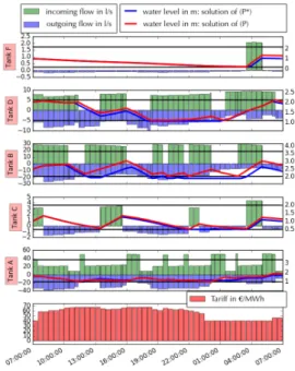
Figure 3 illustrates on instance P21, for each of the 7 pumps of the Poormond network, the optimal pump schedule δ∗ returned by (P∗) after recomputation of the real flows and heads (in blue), and the feasible pump schedule returned by our heuristic (in pink). Figure 4 depicts the water filling profiles of the 5 tanks for both solutions and, below, the dynamic electricity tariff profile.
Figure 3: Approximated and feasible schedules We observe for the approximated solution on Figure 4 that the water levels in the tanks (the blue curves) only slightly fall outside the allowed range (delimited by the black lines) which indicates that the approximated pump schedule is close to be practically feasible. When consid-ering the modelling errors and the security margins and ignoring the formal pump aging constraints, this approx-imated schedule could probably directly be applied as a command for the real-time control of the pumps.
The near feasibility of the solution attests the relevancy of approximating the tank heads to their median values.
Figure 4: Tank levels in the approximated and fea-sible solutions
Indeed, we observe an average relative deviation lower than 1% between the flow profiles delivered by the pumps, before and after recomputation with the actual tank heads. This confirms our hypothesis, we observed on a sample configu-ration, that the error on the flow due to this approximation is significant only when some tanks are empty while oth-ers are full. Here, on the contrary and as expected, the filling profiles of the 5 tanks all follow the same dynamic generated by the variable electricity tariff.
Perhaps more surprising, we observe on Figure 3 that the approximated and feasible pump schedules overlap ex-tensively, from 77% for pump 5C to 100% for pump 1A, which indicates that the approximated solution mostly sat-isfies the fixed time discretization constraint of model (P ) and the pump aging constraints, although they are entirely relaxed in (P∗). Actually, because (P∗) has comparatively few constraints (O(T |J |)), a basic solution has then few columns. In other words, only a fraction of the configu-rations over all the time steps have a non-zero duration in the optimal approximated schedule. For instance P21 depicted here, only 104 configurations are active which corresponds to 3% of the generated configurations, and, on the 48 time steps, 15 are associated to an unique configura-tion. This explains why pumps are activated at reasonable frequency, from 1 for pump 1A to 21 for pump 4B, in the approximated solution.
Finally as the approximated and feasible solutions are close, their costs (111.03 euros for the former and 117.50 for the latter) present a moderate gap (+6%). We observed the same proximity on all the Poormond instances and on all the Van Zyl instances too. For example, in instance Z21, the approximated solution has only 50 active configurations on more than 20,000 candidates over the 48 times steps and it satisfies all the pump aging constraints. Only one iteration of the Benders decomposition and a slight adjustment of
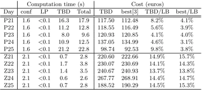
Computation time (s) Cost (euros)
Day conf LP TBD Total TBD best[3] TBD/LB best/LB P21 1.6 <0.1 16.3 17.9 117.50 112.48 8.2% 4.1% P22 1.6 <0.1 11.2 12.8 118.55 116.49 5.6% 3.9% P23 1.6 <0.1 8.0 9.6 120.93 120.85 4.1% 4.0% P24 1.6 <0.1 10.9 12.5 137.05 134.99 4.6% 3.1% P25 1.6 <0.1 21.2 22.8 98.74 92.53 9.8% 3.8% Z21 2.1 <0.1 0.7 2.8 220.60 222.66 14.9% 15.7% Z22 2.1 <0.1 1.7 3.8 230.07 230.69 14.1% 14.3% Z23 2.1 <0.1 1.4 3.5 240.67 240.93 13.7% 13.8% Z24 2.1 <0.1 0.6 2.6 267.77 268.91 14.4% 14.7% Z25 2.1 <0.1 0.7 2.8 188.52 190.29 14.5% 15.3%
Table 1: Results of the heuristic
the pump speeds were needed to retrieve a feasible solution with a +4.2% cost deviation.
5.3
Performance of the heuristic
Table 1 summarizes the computational results of our heuris-tic on the 10 instances of Poormond and Van Zyl. On the left part, the computation times (in seconds) are detailed for each algorithmic component: the preprocessing of the configurations (conf), the solution of the approximated model (P∗) (LP), and the truncated Benders decomposi-tion (TBD). The right part of the table gives the costs (in euros) of the solutions returned by our heuristic (TBD) compared to the solutions of the branch-and-cut approach returned in 1 hour (best [3]); TBD/LB and best/LB de-note the respective optimality gaps to the best know lower bound also returned by the branch-and-cut in 1 hour.
We observe that the heuristic computed good quality solutions fast. About 2 seconds were required to generate an approximated schedule, mostly to preprocess the set of configurations since solving the LP was immediate. The graph partition has a great impact on the number of config-urations to process. On the Van Zyl network, for example, the partition creates two components: the one with all the operable elements but no demand – resulting in 456 configurations which are identical for each time step (even for each instance, actually) – and the other with the unique demand node, only two pipes and no operable elements – resulting in one configuration for each time step. Hence, we computed 456 + 48 hydraulic balances instead of 456 × 48. The truncated Benders decomposition ran in 14 seconds in average on Poormond and in 1 second on Van Zyl. It stopped with a feasible solution after the first iteration, except for instance P25 which required two iterations. On Poormond, the costs of the heuristic solutions were, in average, 2.9% higher than the best solutions, and up to 5% higher for instance P25. In comparison, the branch-and-cut required 306 seconds in average to compute a first feasible solution of comparable quality (at 2.6% of the final solutions). According to [3], our heuristic solutions also improve upon the solutions reported by [6] and [10] after 1 hour of computation. On Van Zyl, the heuristic computed in 3 seconds, in average, solutions which slightly improve upon the solutions found in 1 hour by the branch-and-cut. The average optimality gap is 14.3%. In comparison, [8] reported approximated solutions with a 30% optimality gap computed in 5 minutes by solving a MILP obtained by piecewise linearization of the non-convex constraints in (P ).
6
CONCLUSION
We formulated the pump scheduling problem in water dis-tribution network as a new generic non-compact linear program, based on the approximation of the head at the water tanks and on the relaxation of the pump aging con-straints. This approximation turned out to be both tight and easy to solve when experimented on two networks with different characteristics. We were then able to quickly find low cost feasible solutions by searching in a neighborhood of the approximated solutions. These results lead us to believe that this method could deal with networks larger than with the currently known approaches. Failing to dispose of such study cases, we envisage to build new realistic instances to confirm our claim. Perspectives to extend our method are, first, to exploit the new LP approximation in a global optimization approach, and, second, to exploit historical data of network operations to build the configuration set.
REFERENCES
[1] Bonami, P., Biegler, L., Conn, A., Cornu´ejols, G., Grossmann, I., Laird, C., Lee, J., Lodi, A., Margot, F., and Sawaya, N. An algorithmic framework for convex mixed integer nonlinear programs. Discrete Optimization 5, 2 (2008), 186–204. [2] Bonvin, G., Demassey, S., Le Pape, C., Ma¨ızi, N., Mazauric, V.,
and Samperio, A. A convex mathematical program for pump scheduling in a class of branched water networks. Applied Energy 185 (2017), 1702 – 1711.
[3] Bonvin, G., Demassey, S., and Lodi, A. Pump scheduling in drinking water distribution networks with an LP/NLP-based branch and bound. Tech. rep., CMA, Mines ParisTech, 2018. http://sofdem.github.io/art/bonvin19lpnlp.pdf.
[4] Burgschweiger, J., Gn¨adig, B., and Steinbach, M. Optimiza-tion models for operative planning in drinking water networks. Optimization and Engineering 10, 1 (2009), 43–73.
[5] D’Ambrosio, C., Lodi, A., Wiese, S., and Bragalli, C. Mathe-matical programming techniques in water network optimization. European J. of Operational Research 243, 3 (2015), 774 – 788. [6] Ghaddar, B., Naoum-Sawaya, J., Kishimoto, A., Taheri, N., and Eck, B. A Lagrangian decomposition approach for the pump scheduling problem in water networks. European Journal of Operational Research 241, 2 (2015), 490 – 501.
[7] Mackle, G., Savic, G. A., and Walters, G. A. Application of genetic algorithms to pump scheduling for water supply. In First International Conference on Genetic Algorithms in Engineering Systems: Innovations and Applications (1995), pp. 400–405.
[8] Menke, R., Abraham, E., and Stoianov, I. Modeling variable speed pumps for optimal pump scheduling. In World Environ-mental and Water Resources Congress (2016), pp. 199–209. [9] Morsi, A., Geißler, B., and Martin, A. Mixed integer
optimiza-tion of water supply networks. In Mathematical Optimizaoptimiza-tion of Water Networks. Springer, 2012, pp. 35–54.
[10] Naoum-Sawaya, J., Ghaddar, B., Arandia, E., and Eck, B. Simulation-optimization approaches for water pump scheduling and pipe replacement problems. European Journal of Opera-tional Research 246, 1 (2015), 293–306.
[11] Rossman, L. EPANET, 2000.
[12] Salgado-Castro, R. O. Computer modelling of water supply distribution networks using the gradient method. PhD thesis, Newcastle University, 1988.
[13] Shi, H., and You, F. Energy optimization of water supply system scheduling: Novel MINLP model and efficient global optimization algorithm. AIChE J. 62, 12 (2016), 4277–4296. [14] Single Electricity Market Operator. http://www.sem-o.com.
[accessed: 10-Nov-2016].
[15] Skworcow, P., Paluszczyszyn, D., and Ulanicki, B. Pump schedules optimisation with pressure aspects in complex large-scale water distribution systems. Drinking Water Engineering and Science 7, 1 (2014), 53–62.
[16] Todini, E., and Pilati, S. A gradient algorithm for the analysis of pipe networks. In Computer Applications in Water Supply: Vol. 1—systems Analysis and Simulation, B. Coulbeck and C.-H. Orr, Eds. Research Studies Press Ltd., 1988, pp. 1–20. [17] van Zyl, J., Savic, D., and Walters, G. Operational
opti-mization of water distribution systems using a hybrid genetic algorithm. J. Water Res. Plann. Manage. (2004), 160.