Symbolic Data Analysis: Definition and Examples

SYMBOLIC DATA ANALYSIS: DEFINITIONS

AND EXAMPLES

Universite de Paris 9 Dauphine 75775 Paris Cedex 16 France

Abstract

With the advent of computers, large, very large datasets have become routine. What is not so routine is how to analyse these data and/or how to glean useful information from within their massive confines. One approach is to summarize large data sets in such a way that the resulting summary dataset is of a manageable size. One consequence of this is that the data may no longer be formatted as single values such as is the case for classical data, but may be represented by lists, intervals, distributions and the like. These summarized data are examples of symbolic data. This paper looks at the concept of symbolic data in general, and then attempts to review the methods currently available to analyse such data. It quickly becomes clear that the range of methodologies available draws analogies with developments prior to 1900 which formed a foundation for the inferential statistics of the 1900’s, methods that are largely limited to small (by comparison) data sets and limited to classical data formats. The scarcity of available methodologies for symbolic data also becomes clear and so draws attention to an enormous need for the development of a vast catalogue (so to speak) of new symbolic methodologies along with rigorous mathematical foundational work for these methods.

1

Introduction

With the advent of computers, large, very large datasets have become routine. What is not so routine is how to analyse the attendant data and/or how to glean useful information from within their massive confines. It is evident however that, even in those situations where in theory available methodology might seem to apply, routine use of such statistical techniques is often inappropriate. The reasons are many. Broadly, one reason surrounds the issue of whether or not the data set really is a sample from some populations since oftentimes the data constitute the ”whole”, as, e.g., in the record of all credit transactions of all card users. A related question pertains to whether the data at a specified point in time can be viewed

as being from the same population at another time, as, e.g., will the credit card dataset have the same pattern the next ”week” or when the next week’s transactions are added to the data already collected?

Another major broad reason that known techniques fail revolves around the issue of the shear size of the data set. For example, suppose there are n observations with p variables as-sociated with each individual. Trying to invert an n × n state matrix X when n is measured in the hundreds of thousands or more and p is a hundred or more, whilst theoretically pos-sible, will be computationally heavy. Even as computer capabilities expand (e.g., to invert larger and larger matrices in a reasonable time), these expansions also have a consequence that even larger data sets will be generated. Therefore, while traditional methods have served well on the smaller data sets that dominated in the past, it now behooves us as data analysts to develop procedures that work well on the large modern datasets, procedures that will inform us of the underlying information (or knowledge) inherent in the data.

One approach is to summarize large data sets in such a way that the resulting summary data set is of a manageable size. Thus, in the credit card example instead of hundreds as specific transactions for each person (or credit card) over time, a summary of the transac-tions per card (or, per unit time such as a week) can be made. One such summary format could be a range of transactions by dollars spent (e.g., $10 - $982); or, the summary could be by type of purchase (e.g., gas, clothes, food, ...); or, the summary could be by type and expenditure (e.g., {gas, $10 - $30}, {food, $15 - $95}, ...); or, etc. In each of these examples, the data are no longer single values as in traditional data such as, in this example, $1524 as the total credit card expenditure, or 37 as the total number of transactions, or etc., per person per unit time. Instead, the summarized data constitute ranges, lists, etc., and are therefore examples of symbolic data. In particular, symbolic data have their own internal structure (not present, nor possible, in classical data) and as such should thence be analysed using symbolic data analysis techniques.

While the summarization of very large data sets can produce smaller data sets consisting of symbolic data, symbolic data are distinctive in their own right on any sized data sets small or large. For example, it is not unreasonable to have data consisting of variables each recorded in a range such as pulse rate (e.g., {60, 72}), systolic blood pressure (e.g., {120, 130}) and diastolic blood pressure (e.g., {85, 90}) for each of n = 10 patients (or, for n = 10 million patients). Or, we may have n = 20 students characterized by a histogram or distribution of their marks for each of several variables mathematics, physics, statistics, ..., say. Birds may be characterized by colors e.g., Bird 1 = {black}, Bird 2 = {yellow, blue}, Bird 3 = {half yellow, half red}, ... That is, the variable ’color’ takes not just one possible color for any one bird, but could be a list of all colors or a list with corresponding proportion of each color for that bird. On the other hand, the data point {black} may

indicate a collection of birds all of whom are black; and the point {yellow (.4), red (.6)} may be a collection of birds all of which are 40% yellow and 60% red in color, or a collection of which 40% are entirely yellow and 60% are entirely red, and so on. There are endless examples. In a different direction, we may not have a specific bird(s), but are interested in the concept of a black bird or of a yellow and red bird. Likewise, we can formalize an engineering company as having a knowledge base consisting of the experiences of its employees. Such experiences are more aptly described as concepts rather than as standard data, and as such are also examples of symbolic data. For small symbolic data sets, the question is how the analysis proceeds. For large data sets, the first question is the approach adopted to summarize the data into a (necessarily) smaller data set. Some summarization methods necessarily involve symbolic data and symbolic analysis in some format (while some need not). Buried behind any summarization is the notion of a symbolic concept, with any one aggregation being tied necessarily to the concept relating to a specific aim of an ensuing analysis.

In this work, we attempt to review concepts and methods developed variously under the headings of symbolic data analysis, or the like. In reality, these methods so far have tended to be limited to developing methodologies to organize the data into meaningful and manage-able formats, somewhat akin to the developments leading to frequency histograms and other basic descriptive statistics efforts prior to 1900, which themselves formed a foundation for the inferential statistics of the 1900’s. A brief review of existing symbolic statistical methods is included herein. An extensive coverage of earlier results can be found in Bock and Diday (2000). What quickly becomes clear is that thus far very little statistical methodology has been developed for the resulting symbolic data formats. However, in a different sense, the fundamental exploratory data analyses of Tukey and his colleagues (see, e.g., Tukey, 1977) presages much of what is currently being developed.

Exploratory data analysis, data mining, knowledge discovery in databases, statistics, symbolic data, even fuzzy data, and the like, are becoming everyday terms. Symbolic data analysis extends the ideas in traditional exploratory data analysis to more general and more complex data. Siebes (1998) attempts to identify data mining as the step in which patterns in the data are discovered automatically (using computational algorithms, e.g.), while knowledge discovery covers not only the data mining stage but also preprocessing steps (such as cleaning the data) and post-processing steps (such as the interpretation of the results). Obviously, it is this post-processing stage which has been a traditional role of the statistician. Elder and Pregibon (1996) offer a statistical perspective on knowledge discovery in data bases. Hand et al. (2000) defines data mining ”as the secondary analysis of large databases aimed at finding unsuspected relationships which are of interest or value to the database owners.” The size of the database is such that classical exploratory data

analyses are often inadequate. Since some problems in data mining and knowledge discovery in databases lead naturally to symbolic data formats, symbolic data analyses have a role to play here also. The engagement of cross-disciplinary teams in handling large data sets (such as computer scientists and statisticians) is however becoming essential.

A distinction should also be drawn with fuzzy data and compositional data. Fuzzy data may be represented as the degree to which a given value may hold; see, e.g., Bandemer and Nather (1992), and Viertl (1996). Compositional data (Aitchison, 1986, 1992, 1997) are vectors of nonnegative real components with a constant sum; probability measures or histogram data are a special case with sum equal to one. These types of data can be written as symbolic data by taking into account the variation inside a class of units described by such data and by then using this class as a new unit.

The purpose of this paper is to review concepts of symbolic data and procedures of their analysis as currently available in the literature. Therefore, symbolic data, sometimes called ”atoms of knowledge” so to speak, are defined and contrasted with classical data in Section 2. The construction of classes of symbolic objects, a necessary precursor to statistical analyses when the size of the original data set is too large for classical analyses, or where knowledge (in the form of classes, concepts, taxonomies and so forth) are given as input instead of standard data is discussed in Section 3. In Section 4, we briefly describe available methods of symbolic data analysis, and then discuss some of these in more detail in subsequent sections. What becomes apparent is the inevitability of an increasing prevalence of symbolic data, and hence the attendant need to develop statistical methodologies to analyse such data. It will also be apparent that few methods currently exist, and even for those that do exist the need remains to establish mathematical underpinning and rigor including statistical properties of the results of these procedures. Typically, point estimators have been developed, but there are still essentially no results governing their properties such as standard errors and distribution theory. These remain as outstanding problems.

2

Symbolic Data Sets

A data set may from its outset be structured as a symbolic data set. Alternatively, it may be structured as a classical data set but will become organized as symbolic data in order to establish it in a more manageable fashion, especially when initially it is very large in size. In this section, we present examples of both classical and symbolic data. Also, we introduce notation describing symbolic data sets for analysis. This process includes those situations, e.g., when two or more data sets are being merged, or when different features of the data are to be highlighted.

Suppose we have a data set consisting of the medical records of individuals in a country. Suppose for each individual, there will be a record of geographical location variables, such as

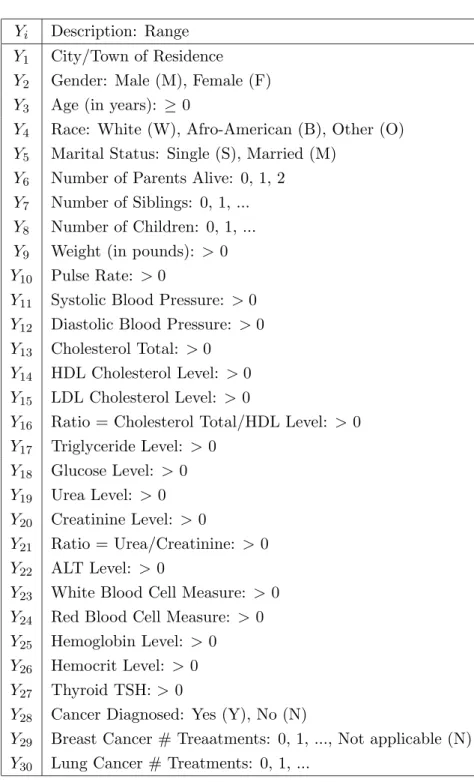
region (north, north-east, south, ...), city (Boston, Atlanta, ...), urban/rural (Yes, No), and so on. There will be demographic variables such as gender, marital status, age, information on parents (alive still, or not) siblings, number of children, employer, health provider, etc. Basic medical variables could include weight, pulse rate, blood pressure, etc. Other health variables (for which the list of possible variables is endless) would include incidences of certain ailments and diseases; likewise, for a given incidence or prognosis, treatments and other related variables associated with that disease are recorded. A typical such data set may follow the lines of Table 1.

Let p be the number of variables for each individual i ∈ Ω = {1, . . . , n}, where clearly p and n can be large, or even extremely large; and let Yj, j = 1, . . . , p, represent the

jth variable. Let Yj = xij be the particular value assumed by the variable Yj for the ith

individual in the classical setting, and write X = (xij) as the n × p matrix of the entire

data set. Let the domain of Yj be Yj; so X = (Y1, . . . , Yp) takes values in X = ×pj=1Yj.

[Since the presence or absence of missing values is of no importance for the present, let us assume all values exist, even though this is most unlikely for large data sets.]

Variables can be quantitative, e.g., age with Yage = {x ≥ 0} = Y+ as a continuous

random variable; or with Yage= {0, 1, 2, . . .} = N0, as a discrete random variable. Variables

can be categorical, e.g., city with Ycity = {Atlanta, Boston, ...} or coded Ycity= {1, 2, . . .},

respectively. Disease variables can be recorded as categories (coded or not) of a single variable with domain Y = {heart, stroke, cancer, cirrhosis, ....}, or, as is more likely, as an indicator variable, e.g., Y = cancer with domain Y = {No, Yes} or {0, 1} or with other coded levels indicating stages of disease. Likewise, for a recording of the many possible types of cancers, each type may be represented by a variable Y , or may be represented by a category of the cancer variable.

The precise nature of the description of the variables is not critical. What is crucial in the classical setting is that for each xij in X, there is precisely one possible realized value.

That is, e.g., an individual’s Yage= 24, say, or Ycity = Boston, Ycancer= Yes, Ypulse = 64, and

so on. Thus, a classical data point is a single point in the p-dimensional space X .

In contrast, a symbolic data point can be a hypercube in p-dimensional space or Carte-sian product of distributions. Entries in a symbolic data set (denoted by ξij) are not

restricted to a single specific value. Thus, age could be recorded as being in an interval, e.g., [0, 10), [10, 20), [20, 30), . . . . This could occur when the data point represents the age of a family or group of individuals whose ages collectively fall in an interval (such as [20, 30) years, say); or the data may correspond to a single individual whose precise age is unknown other than it is known to be within an interval range, or whose age has varied over time in the course of the experiment which generated the data; or combinations and variations thereof, producing interval-ranged data. In a different direction, it may not be possible to

measure some characteristic accurately as a single value, e.g., pulse rate at 64, but rather measures the variable as an (x ± δ) value, e.g., pulse rate is (64 ± 1). A person’s weight may fluctuate between (130, 135) over a weekly period. An individual may have ≤ 2, or > 2 siblings (or children, or ...). The blood pressure variable may be recorded by its [low, high] values, e.g, ξij = [78, 120]. These variables are interval-valued symbolic variables.

A different type of variable would be a cancer variable which may have a domain Y = {lung, bone, breast, liver, lymphoma, prostate, ....} listing all possible cancers with a specific individual having the particular values ξij = {lung, liver}, for example. In another example,

suppose the variable Yj represents type of automobile owned (say) by a household, with

domain {Yj = {Chevrolet, Ford, Toyota, Volvo, . . .}. A particular household i may have

the value ξij = {Toyota, Volvo}. Such variables are called multi-valued variables.

A third type of symbolic variable is a modal variable. Modal variables are multi-state variables with a frequency, probability, or weight attached to each of the specific values in the data. I.e., the modal variable Y is a mapping

Y (i) = {U (i), πi} for i ∈ Ω

where πiis a nonnegative measure or a distribution on the domain Y of possible observation

values and U (i) ⊆ Y is the support of πi. For example, if three of an individual’s siblings

are diabetic and one isn’t, then the variable describing propensity to diabetes could take the particular value ξij = {3/4 diabetes, 1/4 nondiabeties}. More generally, ξij may be

a histogram, an empirical distribution function, a probability distribution, a model, or so on. Indeed, Schweitzer (1984) opined that ”distributions are the numbers of the future”. Whilst in this example the weights (3/4, 1/4) might represent relative frequencies, other kinds of weights such as ”capacities”, ”credibilities”, ”necessities”, ”possibilities”, etc. may be used. Here, we define ”capacity” in the sense of Choquet (1954) as the probability that at least one individual in the class has a certain Y value (e.g., is diabetic); and ”credibility” is defined in the sense of Schafer (1976) as the probability every individual in the class has that characteristic (see, Diday, 1995).

In general then, unlike classical data for which each data point consists of a single (categorical or quantitative) value, symbolic data can contain internal variation and can be structured. It is the presence of this internal variation which necessitates the need for new techniques for analysis which in general will differ from those for classical data. Note however that classical data represent a special case; e.g., the classical point x = a is equivalent to the symbolic interval ξ = [a, a].

Notationally, we have a basic set of objects, which are elements or entities, E = {1, . . . , N } called the object set. This object set can represent a universe of individuals E = Ω (as above) in which case N = n; or if N ≤ n, any one object set is a subset of Ω. Also, as frequently occurs in symbolic analyses, the objects u in E are classes C1, . . . , Cm

of individuals in Ω, with E = {C1, . . . , Cm}, and N = m. Thus, e.g., class C1 may consist

of all those individuals in Ω who have had cancer. Each object u ∈ E is described by p symbolic variables Yj, j = 1, . . . , p, with domain Yj, and with Yj being a mapping from

the object set E to a range Yj which depends on the type of variable Yj is. Thus, if Yj is

a classical quantitative variable, the domain Bj is a subset of the real line <, i.e., Bj ⊆ <;

if Yj is an interval variable, Bj = {[α, β], −∞ < α, β < ∞}; if Yj is categorical (nominal,

ordinal, subsets of a finite domain Yj), then Bj = {B|B ⊆ {(list of cancers, e.g.)}}; and if

Yj is a modal variable, Bj = M (Yj) where M (Y) is family of all nonnegative measures on

Y.

Then, the symbolic data for the object set E are represented by the N × p matrix X = (ξuj) where ξuj = Yj(u) ∈ Bj is the observed symbolic value for the variable Yj,

j = 1, . . . , p, for the object u ∈ E. The row x0

u of X is called the symbolic description of

the object u. Thus, for the data in Table 2, the first row x0

1= {[20, 30], [79, 120], Boston, {Brain tumor}, {Male}, [170, 180]}

represents a male in his 20’s who has a brain tumor, a blood pressure of 120/79, weighs between 170 and 180 pounds and lives in Boston. The object u associated with this x0

u may

be a specific male individual followed over a ten-year period whose weight has fluctuated between 170 and 180 pounds over that interval, or, u could be a collection of individuals whose ages range from 20 to 30 and who have the characteristics described by x0

u. The

data x0

4 in Table 2 may represent the same individual as that represented by the i = 4th

individual of Table 1 but where it is known only that she has either breast cancer (with probability p) or lung cancer (with probability 1−p) but it is not known which. On the other hand, it could represent the set of 47 year old women from El Paso of whom a proportion p have either lung cancer and proportion (1 − p) have breast cancer; or it could represent individuals who have both lung and breast cancer; and so on. (At some stage, whether the variable (Type of Cancer here) is categorical, a list, modal or whatever, would have to be explicitly defined.)

Another issue relates to dependent variables, which for symbolic data implies logical dependence, hierarchical dependence, taxonomic, or stochastic dependence. Logical de-pendence is as the word implies, as in the example, if [age ≤ 10], then [# children = 0]. Hierarchical dependence occurs when the outcome of one variable (e.g., Y2 = treatment for

cancer, say) with Y2 = {chemo, radiation, ...} depends on the actual outcome realized for

another variables (e.g., Y1 = Has cancer with Y1 = {No, Yes}, say). If Y1 has the value

{Yes}, then Y2 = {chemotherapy, say}; while if Y1= {No} then clearly Y2 is not applicable.

[We assume for illustrative purposes here that the individual does not have chemotherapy treatment for some other reason.] In these cases, the non-applicable variable Z is defined with domain Z = {N A}. Such variables are also called mother (Y1)− daughter (Y2)

vari-ables. Other variables may exhibit a taxonomic dependence; e.g., Y1 = region and Y2= city

can take values, if Y1= NorthEast then Y2 = Boston, or if Y1 = South then Y2 = Atlanta,

say.

3

Classes and Their Construction; Symbolic Objects

At the outset, our symbolic data set may already be sufficiently small in size that an appropriate symbolic statistical analysis can proceed directly. An example is the data of Table 11 used to illustrate a symbolic principal component analysis. More generally however and almost inevitably before any real (symbolic) data analysis can be conducted especially for large data sets, there will need to be implemented various degrees of data manipulation to organize the information into classes appropriate to specific questions at hand. In some instances, the objects in E (or Ω) are already aggregated into classes, though even here certain questions may require a reorganization into a different classification of classes regardless of whether the data set is small or large. For example, one set of classes C1, . . . , Cm may represent individuals categorized according to m different types of primary

diseases; while another analysis may necessitate a class structure by cities, gender, age, gender and age, or etc. Another earlier stage is when initially the data are separately recorded as for classical statistical and computer science databases for each individual i ∈ Ω = {1, . . . , n}, with n extremely large; likewise for very large symbolic databases. This stage of the symbolic data analysis then corresponds to the aggregation of these n objects into m classes where m is much smaller, and is designed so as to elicit more manageable formats prior to any statistical analysis. Note that this construction may, but need not, be distinct from classes that are obtained from a clustering procedure. Note also that the m aggregated classes may represent m patterns elicited from a data mining procedure.

This leads us to the concept of a symbolic object developed in a series of papers by Diday and his colleagues (e.g., Diday, 1987, 1989, 1990; Bock and Diday, 2000; and Stephan et al., 2000). We introduce this here first through some motivating examples; and then at the end of this section, a more rigorous definition is presented.

Some Examples

Suppose we are interested in the concept ”Northeasterner”. Thus, we have a description d representing the particular values {Boston, ..., other N-E cities, ...} in the domain Ycity;

and we have a relation R (here ∈)linking the variable Ycity with the particular description

of interest. We write this as [Ycity∈ {Boston, ..., other N-E cities, ...}] = a, say. Then, each

individual i in Ω = {1, . . . , n} is either a Northeasterner or is not. That is, a is a mapping from Ω → {0, 1}, where for an individual i who lives in the Northeast, a(i) = 1; otherwise, a(i) = 0, i ∈ Ω. Thus, if an individual i lives in Boston (i.e., Ycity(i) = Boston), then we

have a(i) =[Boston ⊆ {Boston, . . ., other N-E cities, ...}] = 1.

The set of all i ∈ Ω for whom a(i) = 1, is called the extent of a in Ω. The triple s = (a, R, d) is a symbolic object where R is a relation between the description Y (i) of the (silent) variable Y and a description d and a is a mapping from Ω to L which depends on R and d. (In the Northeasterner example, L = {0, 1}). The description d can be an intentional description; e.g., as the name suggests, we intend to find the set of individuals in Ω who live in the ”Northeast”. Thus, the concept ”Northeasterner” is somewhat akin to the classical concept of population; and the extent in Ω corresponds to the sample of individuals from the Northeast in the actual data set. Recall however that Ω may already be the ”population” or it may be a ”sample” in the classical statistical sense of sampling, as noted in Section 2.

Symbolic objects play a role in one of three major ways within the scope of symbolic data analyses. First, a symbolic object may represent a concept by its intent (e.g., its description and a way for calculating its extent) and can be used as the input of a symbolic data analysis. Thus, the concept ”Northeasterner” can be represented by a symbolic object whose intent is defined by a characteristic description and a way to find its extent which is the set of people who live in the Northeast. A set of such regions and their associated symbolic objects can constitute the input of a symbolic data analysis. Secondly, it can be used as output from a symbolic data analysis as when a clustering analysis suggests Northeasterners belong to a particular cluster where the cluster itself can be considered as a concept and be represented by a symbolic object. The third situation is when we have a new individual (i0_{) who has description d}0_{, and we want to know if this individual (i}0₎

matches the symbolic object whose description is d; that is, we compare d and d0 _{by R to}

give [d0_{Rd] ∈ L = {0, 1}, where [d}0_{Rd] = 1 means that there is a connection between d}0 _and

d. This ”new” individual may be an ”old” individual but with updated data; or it may be a new individual being added to the data base who may or may not ”fit into” one of the classes of symbolic objects already present, (e.g., should this person be provided with specific insurance coverage?).

In the context of the aggregation of our data into a smaller number of classes, were we to aggregate the individuals in Ω by city, i.e., by the value of the variable Ycity, then

the respective classes Cu, u ∈ {1, . . . , m} comprise those individuals in Ω which are in

the extent of the corresponding mapping au, say. Subsequent statistical analysis can take

either of two broad directions. Either, we analyse, separately for each class, the classical or symbolic data for the individuals in Cu as a sample of nu observations as appropriate;

or, we summarize the data for each class to give a new data set with one ”observation” per class. In this latter case, the data set values will be symbolic data regardless of whether the original values were classical or symbolic data. For example, even though each individual

in Ω is recorded as having or not having had cancer (Ycancer = No, Yes), i.e., as a classical

data value, this variable when related to the class for city (say) will become, e.g., {Yes (.1), No (.9)}, i.e., 10% have had cancer and 90% have not. Thus, the variable Ycancer is now a

modal valued variable.

Likewise, a class that is constructed as the extent of a symbolic object, is typically described by a symbolic data set. For example, suppose our interest lies with ”those who live in Boston”, i.e., a = [Ycity = Boston]; and suppose the variable Ychild is the number of

children each individual i ∈ Ω has with possible values {0, 1, 2, ≥ 3}. Suppose the data value for each i is a classical value. (The adjustment for a symbolic data value such as individual i has 1 or 2 children, i.e., ξi = {1, 2}, readily follows). Then, the object representing all

those who live in Boston will now have the symbolic variable Ychild with particular value

Ychild = {(0, f0), (1, f1), (2, f2), (≥ 3, f3)},

where fi, i = 0, 1, 2, ≥ 3, is the relative frequency of individuals in this class who have i

children.

A special case of a symbolic object is an assertion. Assertions, also called queries, are particularly important when aggregating individuals into classes from an initial (relational) database. Let us denote by z = (z1, . . . , zp) the required description of interest of an

individual or of a concept w. Here, zj can be a classical single-valued entity xj or a symbolic

entity ξj. That is, while an xj represents a realized classical data value and ξj represents

a realized symbolic data value, zj is a value being specifically sought or specified. Thus,

for example, suppose we are interested in the symbolic object representing those who live in the Northeast. Then, zcity is the set of Northeastern cities. We formulate this as the

assertion

a = [Ycity∈ {Boston, ..., other N-E cities, ...}] (1)

where a is mapping from Ω to {0, 1} such that, for individual or object w, a(w) = 1 if Ycity(w) ∈ {Boston, ..., other N-E cities, ...}.

In general, an assertion takes the form

a = [Yj1Rj1zj1] ∧ [Yj2Rj2zj2] ∧ . . . ∧ [YjvRjvzjv] (2)

for 1 ≤ j1, . . . , jv ≤ p, where ’∧’ indicates the logical multiplicative ’and’, and R represents

the specified relationship between the symbolic variable Yj and description value zj. For

each individual i ∈ Ω, a(i) = 1 (or 0) when the assertion is true (or not) for that individual. More precisely, an assertion is a conjunction of v events [YkRkzk], k = 1, . . . , v.

For example, the assertions

represent all individuals with cancer, and all individuals aged 60 and over, respectively. The assertion

a = [Ycancer= Yes] ∧ [Yage≥ 60] (4)

represents all cancer patients who are 60 or more years old; while the assertion

a = [Yage< 20] ∧ [Yage > 70] (5)

seeks all individuals under 20 and over 70 years old. In each case, we are dealing with a concept ”those aged over 60”, ”those over 60 with cancer”, etc.; and a maps the particular individuals present in Ω onto the space {0, 1}.

If instead of recording the cancer variable as a categorical {Yes, No} variable, it were recorded as a {lung, liver, breast, ...} variable, the assertion

a = [Ycancer∈ {lung, liver}] (6)

is describing the class of individuals who have either lung cancer or liver cancer or both. Likewise, an assertion can take the form

a = [Yage⊆ [20, 30]] ∧ [Ycity ∈ {Boston}]; (7)

that is, this assertion describes those who live in Boston and are in the 20s age-wise. The relations R can take any of the forms =, 6=, ∈, ≤, ⊆, etc., or can be a matching relationship (such as a comparison of probability distributions), or a structured sequence, and so on. They form the link between the symbolic variable Y and the specific description z of interest. The domain of the symbolic object can be written as,

D = D1× . . . × Dp ⊆ X = ×pj=1Yj.

where Dj ⊆ Yj. The p-tuple (D1, . . . , Dp) of sets is called a description system, and each

subset D is a description set consisting of description vectors z = (z1, . . . , zp); while a

combination of elements zj ∈ Yj and sets Dj ⊆ Yj as in (7) above for example is simply

a description. When there are constraints on any of the variables (such as when logical dependencies exist), then the space D has a ”hole” in it corresponding to those values which match the constraints. The totality of all descriptions D is the description space D. Hence, the assertion can be written as

a = [Y ∈ D] ≡ v ^ k=1 [YjkRjkzjk] = [Y Rz] where R =Vv

k=1Rjk is called the product relation.

Note that implicitly, if an assertion does not involve a particular variable Yw, say, then

Y1 = city, Y2 = age and Y3 = weight, then the assertion a = [Y1 ∈ {Boston, Atlanta}] has

domain D = {Boston, Atlanta} × Y2× Y3 and seeks all those in Boston and Atlanta only

(but regardless of age and weight). Formal Definitions

Let us now formally define the following concepts.

Definition: When an assertion is asked of any particular object i ∈ Ω, it assumes a value true (a = 1) if that assertion holds for that object, or false (a = 0) if not. We write

a(i) = [Y (i) ∈ D] =

(

1, Y (i) ∈ D,

0, otherwise. (8) The function a(i) is called a truth function and represents a mapping of Ω onto {0, 1}. The set of all i ∈ Ω for which the assertion holds is called the extension in Ω, denoted by Ext(a) or Q,

Ext(a) = Q = {i ∈ Ω|Y (i) ∈ D} = {i ∈ Ω|a(i) = 1}. (9) Formally, the mapping a : Ω → {0, 1} is called an extension mapping.

Typically, a class would be identified by the symbolic object that described it. For exam-ple, the assertion (7) corresponds to the symbolic object ”20-30 year olds living in Boston”. The extension of this assertion, Ext(a), produces the class consisting of all individuals i ∈ Ω which match this description a, i.e., those i for whom a(i) = 1.

A class may be constructed, as in the foregoing, by seeking the extension of an assertion a. Alternatively, it may be that it is desired to find all those (other) individuals in Ω who match the description Yj(u) of a given individual u ∈ Ω. Thus in this case, the assertion is

a(i) =

p

^

j=1

[Yj = Yj(u)]

where now zj = Yj(u), and has extension

Ext(ai) = {i ∈ Ω|Yj(i) = Yj(u), j = 1, . . . , p}.

More generally, an assertion may hold with some intermediate value (such as a proba-bility), i.e., 0 ≤ a(i) ≤ 1, representing a degree of matching of an object i with an assertion a. Flexible matching is also possible. In these cases, the mapping a is onto the interval [0, 1], i.e., a : Ω → [0, 1]. Then, the extension of a has level α, 0 ≤ α ≤ 1, where now

Extα(a) = Qα = {i ∈ Ω|a(i) ≥ α}.

Diday and Emilion (1996) and Diday et al. (1996) study modal symbolic objects and also provide some of its theoretical underpinning; see also Section 10.

We now have the formal definition of a symbolic object as follows.

Definition: A symbolic object is the triple s = (a, R, d) where a is a mapping a : Ω → L which maps individuals i ∈ Ω onto the space L depending on the relation R between descriptions and the description d. When L = {0, 1}, i.e., when a is a binary mapping, then s is a Boolean symbolic object. When L = [0, 1], then s is a modal symbolic object. That is, a symbolic object is a mathematical model of a concept (see, Diday, 1995). If [a, R, d] ∈ {0, 1}, then s is a Boolean symbolic object and if [a, R, d] ∈ [0, 1], then s is a modal symbolic object. For example, in (7) above, we have the relations R = (⊆, ∈) and the description d = ([20, 30], {Boston}). The intent is to find ”20-30 year olds who live in Boston”. The extent consists of all individuals in Ω who match this description, i.e., those i for whom a(i) = 1.

Whilst recognition of the need to develop methods for analyzing symbolic data and tools to describe symbol objects is relatively new, the idea of considering higher level units as concepts is in fact ancient. Aristotle Organon in the 4th century BC (Aristotle, IVBC, 1994) clearly distinguishes first order individuals (such as the horse or the man) which represented units in the world (the statistical population) from second order individuals (such as a horse or a man) represented as units in a class of individuals. Later, Arnault and Nicole (1662) defined a concept by notions of an intent and an extent (whose meanings in 1662 match those herein) as: ”Now, in these universal ideas there are two things which is important to keep quite distinct: comprehension and extension (for ”intent” and ”extent”). I call the comprehension of an idea the attributes which it contains and which cannot be taken away from it without destroying it; thus the comprehension of the idea of a triangle includes, to a superficial extent, figure, three lines, three angles, the equality of these three angles to two right angles etc. I call the extension of an idea the subjects to which it applies, which are also called the inferiors of a universal term, that being called superior to them. Thus the idea of triangle in general extends to all different kinds of triangle”.

Finally, computational implementation of the generation of appropriate classes can be executed by queries (assertions) used in search engines such as the exhaustive search, genetic, or hill climbing algorithms, and/or by the use of available software such as the standard query language (SQL) package or other ”object oriented” languages such as C++or JAVA. Stephan et al. (2000) provide some detailed examples illustrating the use of SQL. An-other package specifically written for symbolic data is the SODAS (Symbolic Official Data Analysis System) software. Gettler-Summa (1999, 2000) developed the MGS (marking and generalization by symbolic descriptions algorithm) for building symbolic descriptions start-ing with classical nominal data. Thus, the outputs (ready for symbolic data analysis) are symbolic objects which have modal or multi-valued variables and which identify logical

links between the variables. Csernel (1997), inspired by Codd’s (1972) methods of deal-ing with relational databases with functional dependencies between variables, developed a normalization of Boolean symbolic objects taking into account constraints on the variables. While we have not addressed it explicitly, the concepts described in this section can also be applied to merged or linked data sets. For example, suppose we also had a data set consisting of meteorological and environmental variables (measured as classical or symbolic data) for cities in the U.S. Then, if the data are merged by city, it is easy to obtain relevant meteorological and environmental data for each individual identified in Table 1. Thus, for example, questions relating to environmental measures and cancer incidences could be considered.

4

Symbolic Data Analyses

Given a symbolic data set, the next step is to conduct statistical analyses as appropriate. As for classical data, the possibilities are endless. Unlike classical data for which a century of effort has produced a considerable library of analytical/statistical methodologies, symbolic statistical analyses are new and available methodologies are still only few in number. In the following sections, we shall review some of these as they pertain to symbolic data.

Therefore, in Sections 5 and 6, we consider descriptive statistics. Then, we review principal component methods for interval-valued data in Section 7. Clustering methods are treated in Section 8. Attention will be restricted to the more fully developed criterion-based divisive clustering approach for categorical and interval-valued variables. A summary of other methods limited largely to specific special cases will also be provided. Much of the current progress in symbolic data analyses revolve around cluster-related questions. Theoretical underpining where it exists is covered in Section 9.

Except for the specific distance measures developed for symbolic clustering analysis (see Section 8), we shall not attempt herein to review the literature on symbolic similarity and dissimilarity measures. Classical measures include the Minkowski or Lq distance (with

q = 2 being the Euclidean distance measure), Hamming distance, Mahalanobis distance, and Gower-Legendre family, plus the large class of dissimilarity measures for probability distributions from classical probability and statistical theory, e.g., the familiar chi-square measure, Bhattacharyya distance and Chernoff’s distance, to name but a very few. Symbolic analogues have been proposed for specific cases. Gowda and Diday (1991) first introduced a basic dissimilarity measure for Boolean symbolic objects. Later, Ichino and Yaguchi (1994), using Cartesian operators, developed a symbolic generalized Minkowski distance of order q ≥ 1. This was extended by De Carvalho (1994, 1998) to include Boolean symbolic ob-jects constrained by logical dependencies between variables. Matching of Boolean symbolic objects is considered by Esposito et al. (1991). These measures invoke the concepts of

Cartesian join, and meet. Some are developed along the lines of distance functions (as de-scribed in Section 8; see, e.g., Chavent, 1998). Many are limited to univariate cases. Since such measures vary widely and the choices of what to use are generally dependent on the task at hand, we shall not expand on their details further. In a different direction, Morineau et al. (1994), Loustaunau et. al. (1997) and Gettler-Summa and Pardoux (2000) consider three-way tables. A more detailed and exhaustive description of symbolic methodologies in general up to its publication can be found in Bock and Diday (2000). Billard and Diday (2002b) also has an expanded coverage providing some additional illustrations.

5

Descriptive Univariate Statistics

5.1 Some preliminaries

Basic descriptive statistics include frequency histograms, and sample means and vari-ances. We consider symbolic data analogues of these statistics, for multi-valued and interval-valued variables with rules and modal variables. As we develop these statistics, let us bear in mind the following example which illustrates the need to distinguish between the levels (e.g., structure) in symbolic data when constructing (e.g.) histograms compared with that for a standard histogram.

Suppose an isolated island contains one thousand penguins and one thousand ostriches both non-flying species of birds, and four thousand pigeons which is a flying bird species. Suppose we are interested in the variable ”flying” which here takes two possible values ”Yes” or ”No”. Then, a standard histogram based on birds is such that the frequency for ”Yes” is two times higher than that for ”No”; see Figure 1(a). In contrast, if we consider the individuals to be the species, then since there are two non-flying species and one flying species, the frequency for ”No” is now two times higher than it is for ”Yes”; see Figure 1(b). Notice that a histogram of species is just a histogram. What this example shows is that depending on the level of individuals (here birds) and on the level of concept (here species) we obtain completely different histograms. Species here actually has within it another level of information corresponding to the type of bird and the frequency of each. That is, ”species” itself contains structure at another level from the variable species as used to produce the histogram of Figure 1(b). A symbolic histogram (developed later in this section) takes this structure into account.

We consider univariate statistics (for the p ≥ 1 variate data) in this section and bivari-ate statistics in Section 6. For integer-valued and interval-valued variables, we follow the approach adopted by Bertrand and Goupil (2000). DeCarvalho (1994, 1995) and Chouakria et al. (1998) have used different but equivalent methods to find the histogram and interval probabilities (see equation (26) below) for interval-valued variables.

Before describing these quantities, we first need to introduce the concept of virtual extensions. Recall from Section 3 that the symbolic description of an object u ∈ E (or equivalently, i ∈ Ω) was given by the description vector du = (ξu1, . . . , ξup), u = 1, . . . , m,

or more generally, d ∈ (D1, . . . , Dp) in the space D = ×pj=1Dj, where in any particular case

the realization of Yj may be an xj as for classical data or an ξj of symbolic data. Individual

descriptions, denoted by x, are those for which each Dj is a set of one value only, i.e.,

x ≡ d = ({x1}, . . . , {xp}), x ∈ X = ×pj=1Yj.

The calculation of the symbolic frequency histogram involves a count of the number of individual descriptions that match certain implicit logical dependencies in the data. A logical dependency can be represented by a rule v,

v : [x ∈ A] ⇒ [x ∈ B] (10) for A ⊆ D, B ⊆ D, and x ∈ X and where v is a mapping of X onto {0, 1} with v(x) = 0(1) if the rule is not (is) satisfied by x. For example, suppose x = (x1, x2) = (10, 0) is an

individual description of Y1 = age and Y2 = number of children for i ∈ Ω, and suppose

A = {age ≤ 12} and B = {0}. Then, the rule that an individual whose age is less than 12 implies they have had no children is logically true, whereas an individual whose age is under 12 but has had 2 children is not logically true. It follows that an individual description vector x satisfies the rule v if and only if x ∈ A ∩ B or x /∈ A. This formulation of the logical dependency rule is sufficient for the purposes of establishing basic descriptive statistics. Verde and DeCarvalho (1998) discuss a variety of related rules (such as logical equivalence, logical implication, multiple dependencies, hierarchical dependencies, and so on). We have the following formal definition.

Definition: The virtual description of the description vector d as the set of all individual description vectors x that satisfy all the (logical dependency) rules v in X . We write this as, for Vx the set of all rules v operating on x,

vir(d) = {x ∈ D; v(x) = 1, for all v in Vx}. (11)

5.2 Multi-valued Variables - Univariate Statistics

Suppose we want to find the frequency distribution for the particular multivalued sym-bolic variable Yj ≡ Z which takes possible particular values ξ ∈ Z. These can be categorical

values (e.g., types of cancer), or any form of discrete random variable. We define the ob-served frequency of ξ as

OZ(ξ) =

X

u∈E

πZ(ξ; u) (12)

where the summation is over u ∈ E = {1, . . . , m} and where πZ(ξ; u) =

|{x ∈ vir(du)|xZ= ξ}|

|vir(du)|

is the percentage of the individual description vectors in vir(du) such that xZ = ξ, and

where |A| is the number of individual descriptions in the space A. In the summation in (12), any u for which vir(du) is empty is ignored. We note that this observed frequency is

a positive real number and not necessarily an integer as for classical data. In the classical case, |vir(du)| = 1 and so is a special case of (13). We can easily show that

X

ξ∈Z

OZ(ξ) = m0 (14)

where m0_{= (m − m}

0) with m0 being the number of u for which |vir(du)| = 0.

For a multi-valued symbolic variable Z, taking values ξ ∈ Z, the empirical frequency distribution is the set of pairs [ξ, OZ(ξ)] for ξ ∈ Z, and the relative frequency

distri-bution or frequency histogram is the set

[ξ, (m0)−1OZ(ξ)]. (15)

The following definitions follow readily.

The empirical distribution function of Z is given by FZ(ξ) = 1 m0 X ξk≤ξ OZ(ξk). (16)

When the possible values ξ for the multi-valued symbolic variable Yj = Z are

quantita-tive, we can define a symbolic mean, variance, and median, as follows. The symbolic sample mean is

¯ Z = 1 m0 X ξk ξkOZ(ξk); (17)

the symbolic sample variance is S_Z2 = 1

m0

X

ξk

OZ(ξk)[ξk− ¯Z]2; (18)

and, the symbolic median is the value ξ for which

FZ(ξ) ≥ 1/2, FZ(ξ−≤ 1/2). (19)

An Example

To illustrate, suppose a large data set (consisting of patients served through a particular HMO in Boston, say) was aggregated in such a way that it produced the data of Table 3 representing the outcomes relative to the presence of cancer Y1 with Y1 = {No= 0, Yes =

1} and Number of cancer related treatments Y2 with Y2 = {0, 1, 2, 3} on m = 9 objects.

for the individuals represented by this description, the observation Y1 = {0, 1} tells us

that either some individuals have cancer and some do not or we do not know the precise Yes/No diagnosis for the individuals classified here, while the observation Y2 = {2} tells

us all individuals represented by d1 have had two cancer related treatments. In contrast,

d7 = ({1}, {2, 3}) represents individuals all of whom have had a cancer diagnosis (Y1 = 1)

and who have had either 2 or 3 treatments, Y2 = {2, 3}. Suppose further there is a logical

dependency

v : y1∈ {0} ⇒ y2= {0}, (20)

i.e., if no cancer has been diagnosed, then there must have been no cancer treatments. Notice that y1 ∈ {0} ⇒ A = {(0, 0), (0, 1), (0, 2)(0, 3)} and y2 ∈ {0} ⇒ B = {(0, 0), (1, 0), (2, 0),

(3, 0)}. From (20), it follows that an individual description x which satisfies this rule is x ∈ A ∩ B = {(0, 0)} or x /∈ A, i.e., x ∈ {(1, 0), (1, 1), (1, 2), (1, 3)}. Let all possible cases that satisfy the rule be represented by C = {(0, 0), (1, 0), . . . , (1, 3)}. We apply (20) to each du, u = 1, . . . , m, in the data to find the virtual extensions vir(du). Thus, for the first

description d1, we have

vir(d1) = {x ∈ {0, 1} × {2} : v(x) = 1}.

The individual descriptions x ∈ {0, 1}×{2} are (0,2) and (1,2), of which only one, x = (1, 2), is also in the space C. Therefore, vir(d1) = {(1, 2)}.

Clearly then, this operation is mathematically cleaning the data (so to speak) by identi-fying only those values which make logical sense (by satisidenti-fying the logical dependency rule of equation (20)). Thus, the data values (Y1, Y2) = (0, 2) which record that both no cancer

was present and there were two cancer related treatments are identified as erroneous data values (under the prevailing circumstances as specified by the rule v) and so are not used in this analyis to calculate the mean. [While not attempting to do so here, this identification does not preclude inclusion of other procedures which might subsequently be engaged to imput what these values might have been.] For small data sets, it may be possible to ”cor-rect” the data visually (or some such variation thereof). For very large data sets, this is not always possible; hence a logical dependency rule to do so mathematically/computationally is essential.

Similarly, for the second description d2, we can obtain

vir(d2) = {x ∈ {0, 1} × {0, 1} : v(x) = 1}.

Here, the individual description vectors x ∈ {0, 1} × {0, 1} are (0,0), (0,1), (1,0) and (1,1) of which x = (0, 0), x = (1, 0) and x = (1, 1) are in C. Hence, vir(d2) = {(0, 0), (1, 0), (1, 1)}.

The virtual extensions for all du, u = 1, . . . , 9, are shown in Table 3. Notice that vir(d5) = φ

We can now find the frequency distribution. Suppose we first find this distribution for Y1. By definition (12), we have observed frequencies

OY1(0) = X u∈E0 |{x ∈ vir(du)|xY1 = 0}| |vir(du)| = 0 1 + 1 3 + 0 1 + 0 2+ 1 1+ 0 2 + 0 2 + 0 2 = 4/3, and, likewise, OY1(1) = 20/3, where E

0 _{= E − (u = 5) and so |E}0_{| = 8 = m}0_{. Therefore, the}

relative frequency distribution for Y1 is, from equation (15),

Rel freq (Y1) : [(0, OY1(0)/m

0

), (1, OY1(1)/m

0

)] = [(0, 1/6), (1, 5/6)].

Similarly, we have observed frequencies for the possible Y2 values ξ = 0, 1, 2, 3,

respec-tively, as OY2(0) = X u∈E0 |{x ∈ vir(du)|xY2 = 0}| |vir(du)| = 0 1 + 2 3+ 0 1 + 0 2 + 1 1 + 0 2+ 0 2+ 0 2 = 5/3, OY2(1) = 4/3, OY2(2) = 2.5, OY2(3) = 2.5;

and hence, the relative frequency for Y2 is, from equation (15),

Rel freq (Y2) : [(0, 5/24), (1, 1/6), (2, 5/16), (3, 5/16)].

The empirical distribution function for Y2 is, from equation (16),

FY2(ξ) =              5/24, ξ < 1, 3/8, 1 ≤ ξ < 2, 11/16, 2 ≤ ξ < 3, 1, ξ ≥ 3.

From equation (17), we have that the symbolic sample mean of Y1 and Y2, respectively,

is ¯Y1 = 5/6 = 0.833 and ¯Y2 = 83/48 = 1.729; from equation (18), the symbolic sample

variance of Y1 and Y2, respectively, is S21 = 0.1239 and S22 = 1.1975 respectively; and the

median of Y2 is 2.

Finally, we observe that we can calculate weighted frequencies, weighted means and weighted variances by replacing (12) by

OZ(ξ) =

X

u∈E

wuπZ(ξ, u) (21)

with wu ≥ 0 and Σwu = 1. For example, if the objects u ∈ E are classes Cu comprised

wu = |Cu|/|Ω| corresponding to the relative sizes of the class Cu, u = 1, . . . , m. Or, more

generally, if we consider each individual description vector x as an elementary unit of the object u, we can use weights, for u ∈ E,

wu =

|vir(du)|

P

u∈E|vir(du)|

. (22)

For example, if the u of Table 3 represent classes Cu of size |Cu|, with |Ω| = 1000, as

shown in Table 3, then, if we use the weights wu = |Cu|/|Ω|, we can show that

OY1(0) = 1 1000[128 × 0 1 + 75 × 1 3 + 249 × 0 1 + . . . + 121 × 0 2] = 0.229; likewise, OY1(1) = 0.771.

Hence, the relative frequency of Y1 is

Rel freq (Y1) : [(0, 0.229), (1, 0.771)].

Likewise,

OY2(0) = 0.2540, OY2(1) = 0.0970, OY2(2) = 0.2395, OY2(3) = 0.4095;

and hence the relative frequency of Y2 is

Rel freq (Y2) : [(0, 0.2540), (1, 0.0970), (2, 0.2395), (3, 0.4095)].

The empirical weighted distribution function for Y2 becomes

FY2(ξ) =              0.2540, ξ < 1, 0.3510, 1 ≤ ξ < 2, 0.5905, 2 ≤ ξ < 3, 1, ξ ≥ 3.

Similarly, we can show that the symbolic weighted sample mean of Y1 is ¯Y1 = 0.7710 and

of Y2 is ¯Y2= 1.8045, and the symbolic weighted sample variance of Y1 is ξ12 = 0.176 and of

Y2 is S22 = 1.4843.

5.3. Interval-valued Variables - Univariate Statistics

The corresponding description statistics for interval-valued variables are obtained anal-ogously to those for multi-valued variables; see Bertrand and Goupil (2000). Let us suppose we are interested in the particular variable Yj ≡ Z, and suppose the observation value for

object u is the interval Z(u) = [au, bu], for u ∈ E = {1, . . . , m}. The individual

descrip-tion vectors x ∈ vir(du) are assumed to be uniformly distributed over the interval Z(u).

Therefore, it follows that, for each ξ,

P {x ≤ ξ|x ∈ vir(du)} =        0, ξ < au, ξ−au bu−au, au ≤ ξ < bu, 1, ξ ≥ bu. (23)

The individual description vector x takes values globally inS

u∈Evir(du). Further, it is

assumed that each object is equally likely to be observed with probability 1/m. Therefore, the empirical distribution function, FZ(ξ), is the distribution function of a mixture of m

uniform distributions {Z(u), u = 1, . . . , m}. Therefore, from (23), FZ(ξ) = 1 m X u∈E P {x ≤ ξ|x ∈ vir(du)} = 1 m    X ξ∈Z(u) µ_{ξ − a} u bu− au ¶ + |(u|ξ ≥ bu)|    .

Hence, by taking the derivative with respect to ξ, we obtain the empirical density func-tion of Z as f (ξ) = 1 m X u:ξ∈Z(u) µ ₁ bu− au ¶ . (24)

Notice that the summation in (24) is only over those objects u for which ξ ∈ Z(u). We may write (24) in the alternative form

f (ξ) = 1 m X u∈E Iu(ξ) ||Z(u)||, ξ ∈ <, (25) where Iu(.) is the indicator function that ξ is or is not in the interval Z(u) and where

||Z(u)|| is the length of that interval. Note that the summation in (25) is only over those objects u for which ξ ∈ Z(u). The analogy with (15) and (16) is apparent.

To construct a histogram, let I = [minu∈Eau, maxu∈Ebu] be the interval which spans

all the observed values of Z in X , and suppose we partition I into r subintervals Ig =

[ξg−1, ξg), g = 1, . . . , r − 1, and Ir = [ξr−1, ξr]. Then, the histogram for Z is the graphical

representation of the frequency distribution {(Ig, pg), g = 1, . . . , r} where

pg = 1 m X u∈E ||Z(u) ∩ Ig|| ||Z(u)|| , (26)

i.e., pg is the probability an arbitrary individual description vector x lies in the interval Ig.

If we want to plot the histogram with height fg on the interval ig, so that the ”area” is pg,

then

Bertrand and Goupil (2000) indicate that, using the law of large numbers, the true limiting distribution of Z as m → ∞ is only approximated by the exact distribution f (ξ) in (25) since this depends on the veracity of the uniform distribution within each interval assumption. Mathematical underpining for the histogram has been developed in Diday (1995) using the strong law of large numbers and the concepts of t-norms and t-conorms as developed by Schweizer and Sklar (1983).

The symbolic sample mean, for an interval-valued variable Z, is given by ¯ Z = 1 2m X u∈E (bu+ au), (28)

To verify (28), we recall the empirical mean ¯Z in terms of the empirical density function is ¯

Z =

Z ∞

−∞

ξf (ξ)dξ. Substituting from (25), we have

¯ Z = 1 m X u∈E Z ∞ −∞ Iu(ξ) ||Z(u)||ξdξ = 1 m X u∈E 1 bu− au Z ξ∈Z(u) ξdξ = 1 2m X u∈E b2_u− a2 u bu− au = 1 m X u∈E (bu+ au)/2, as required.

Similarly, we can derive the symbolic sample variance given by S2 = 1 3m X u∈E (b2_u+ buau+ a2u) − 1 4m2[ X u∈E (bu+ au)]2. (29)

As for multi-valued variables, if an object u has some internal inconsistency relative to a logical rule, i.e., if u is such that |vir(du)| = 0, then the summation in (28) and (29) is

over only those u for which |vir(du)| 6= 0, i.e., over u ∈ E0, and m is replaced by m0 (equal

to the number of objects u in E0_{). In the sequel, it will be understood that m and E refer}

to those u for which these rules hold. An Example

To illustrate, consider the data from Raju (1997) shown in Table 4, in which the pulse rate (Y1), systolic blood pressure (Y2) and diastolic blood pressure (Y3) are recorded as an

interval for each of the u = 1, . . . , 10 patients. Let us take the data for pulse rate (Y1). The

complete data set spans an interval I = [44, 112] where min

u∈Eau = 44, maxu∈Ebu= 112.

Suppose we want to construct a histogram on the r = 8 intervals I1 = [40, 50), . . . , I8 =

[110, 120]. Using equation (26), we can calculate the probability pg that an arbitrary

indi-vidual description vector x lies in the interval Ig, g = 1, . . . , 8. For example, when g = 4,

the probability that an x lies in the interval I4= [70, 80) is

p4= 1 10{0 + 2 12+ 10 34+ 10 42+ 2 18 + 10 30 + 8 28 + 4 22 + 0 + 0} = .1611.

Hence, from equation (27), we can calculate the height fg of the plotted histogram for that

interval as

fg = pg/(ξg− ξg−1)

i.e.,

f4 = (.1611)/10 = .01611.

A summary of the calculated values of pg for each Ig is given in Table 5, and the plot of

the histogram is shown in Figure 2. Table 5 also provides the intervals and probabilities for the interval valued variable Y2 which represents the systolic blood pressure and for Y3

which represents the diastolic blood pressure for the same ten patients.

Using the equations (28) and (29), we find the symbolic sample mean and variance respectively. Thus, the mean pulse rate is ¯Y1 = 79.1 with variance S12 = 215.86; the mean

systolic blood pressure is ¯Y2 = 131.3 with variance S22 = 624.18; and the mean diastolic

blood pressure is ¯Y3 = 84.6 with variance S32 = 229.64.

5.4 Multi-valued Modal Variables

There are many types of modal-valued variables. We consider very briefly two types only, one each of multi-valued and interval valued variables in this subsection and the next (5.5), respectively.

Let us suppose we have data from a categorical variable Yj taking possible values ξjk,

with relative frequencies pk, k = 1, . . . , s, respectively, with Σpk= 1. Suppose we are

inter-ested in the particular symbolic random variable Yj ≡ Z, in the presence of the dependency

rule v. Then, we define the observed frequency that Z = ξk, k = 1, . . . , s, as

OZ(ξk) =

X

u∈E

πZ(ξk; u) (30)

where the summation is over all u ∈ E and where

= P xP (x = ξk|v(x) = 1, u) P xPsk=1P (x = ξk|v(x) = 1, u) (31) where, for each u, P (x = ξk|v(x) = 1, u) is the probability that a particular description x

(≡ xj) has the value ξkand that the logical dependency rule v holds. If for a specific object

u, there are no description vectors satisfying the rule v, i.e., if the denominator of (31) is zero, then that u is omitted in the summation in (30). We note that

s

X

k=1

OZ(ξk) = m. (32)

An example

Suppose households are recorded as having one of the possible central heating fuel types Y1 taking values in Y1 = {gas, solid fuel, electricity, other} and suppose Y2 is an

indicator variable taking values in Y1 = {No, Yes} depending on whether a household

does not (does) have central heating installed. For illustrative convenience, it is assumed the values for Y1 are conditional on there being central heating present in the household.

Suppose that aggregation by geographical region produced the data of Table 6. The original (classical) data set consisted of census data from the UK Office for National Statistics on 34 demographic-socio-economic variables on individual households in 374 parts of the country. The data shown in Table 6 are those obtained for two specific variables after aggregation into 25 regions; and were obtained by applying the Symbolic Official Data Analysis System software to the original classical data set. Thus, region one represented by the object u = 1 is such that 87% of the households with central heating are fueled by gas, 7% by solids, 5% by electricity and 1% by some other type of fuel; and that 9% of households did not have central heating while 91% did. Let us suppose interest centers only on the variable Y1

(without regard to any other variable) and that there is no rule v to be satisfied. Then, it is readily seen that the observed frequency that Z = ξ1 = gas is

OY1(ξ1) = (0.87 + . . . + 0.43 + 0.00) = 18.05,

and likewise, for ξ2= solid, ξ3 = electricity, and ξ4 = other fuels, we have, respectively,

OY1(ξ2) = 1.67, OY1(ξ3) = 3.51, OY1(ξ4) = 1.77.

Hence, the relative frequencies are

Rel freq (Y1) : [(ξ1, 0.722), (ξ2, 0.067), (ξ3, 0.140), (ξ4, 0.071)].

Similarly, we can show that for the Y2 variable,

Suppose however there is the logical rule that a household must have one of ξk, k =

1, . . . , 4, if it has central heating. For convenience, let us denote Y1 = ξ0 if there is no fuel

type used. (That is, Y1 = ξ0 corresponds to Y2 = No). Then, this logical rule can be written

as the pair v = (v1, v2) v = ( v1: y2 ∈ {No} ⇒ y1∈ {ξ0}, v2: y2 ∈ {Yes} ⇒ y1 ∈ {ξ1, . . . , ξ4}. (33) Let us suppose the relative frequencies for both Y1 and Y2 pertain as in Table 7 (that is,

with the ξ0 values having zero relative frequencies) except that the values for the original

object u = 25, are replaced by the new relative frequencies for Y1 of (.25, .00, .41, .14, .20),

respectively. We will refer to this as object u = 25∗_.

Let us consider Y1 and u = 25∗. In the presence of the rule v, the particular descriptions

x = (Y1, Y2) ∈ {(ξ0, No), ξ1, Yes), (ξ2, Yes), (ξ3, Yes), (ξ4, Yes)} can occur. Thus, the

relative frequencies for each of the possible ξk values have to be adjusted.

Table 7 displays the apparent relative frequencies for each of the possible description vectors before any rules have been invoked. Those values indicated by a0₊0 _{are those which}

are invalidated after invoking the rule v. Let us consider the relative frequency for ξ2 (solid

fuels). Under the rule v, the adjusted relative frequency for object u = 25∗ _is

πY1(ξ2; 25

∗_{) = (.3731)/[.0225 + . . . + .1820] = .5292.}

Hence, the observed frequency for ξ2 over all objects becomes under v

OY1(ξ2) = .0637 + . . . + .0000 + .5292 = 1.5902.

Similarly, we calculate under v that

OY1(ξ0) = 3.8519, OY1(ξ1) = 15.2229, OY1(ξ3) = 2.9761, OY1(ξ4) = 1.3589.

It is readily seen that the summation of (32) holds, with m = 25. Hence, the relative frequencies for Y1 are

Rel freq(Y1) : [(ξ0, 0.154), (ξ1, 0.609), (ξ2, 0.064), (ξ3, 0.119), (ξ4, 0.054)].

Likewise, we can show that the relative frequencies for Y2 are

Rel freq(Y2) : [(No, 0.154), (Yes, 0.846)].

Therefore, over all regions, 60.9% of households use gas, 6.4% use solid fuel, 11.9% use electricity and 5.4% use other fuels to operate their central heating systems, while 15.4% do not have central heating.

For the original data values for u = 25, we can obtain the respective relative frequencies, respectively, as

Rel freq(Y1) : [(ξ0, 0.156), (ξ1, 0.609), (ξ2, 0.057), (ξ3, 0.117), (ξ4, 0.060)];

and

Rel freq(Y2) : [(No, 0.156), (Yes, 0.844)].

5.5 Interval-valued Modal Variables

Let us suppose the random variable of interest, Z ≡ Y for object u, u = 1, . . . , m, takes values on the intervals ξuk = [auk, buk) with probabilities puk, k = 1, . . . , su. One

manifestation of such data would be when (alone, or after aggregation) an object u assumes a histogram as its observed value of Z. An example of such a data set would be that of Table 8, in which the data (such as might be obtained from Table 1 after aggregation) display the histogram of weight of women by age-groups (those aged in their 20s, those in their 30s, ..., those in their 80s and above). Thus, for example, we observe that for women in their thirties (object u = 2), 40% weigh between 116 and 124 pounds. Figure 3 displays the histograms for the respective age groups.

By analogy with ordinary interval-valued variables (see Section 5.3), it is assumed that within each interval [auk, buk), each individual description vector x ∈ vir(du) is uniformly

distributed across that interval. Therefore, for each ξk,

P {x ≤ ξk|x ∈ vir(du)} =        0, ξk< auk, ξk−auk buk−auk, auk ≤ ξk< buk, 1, k ≥ buk. (34)

A histogram of all the observed histograms can be constructed as follows. Let I = [ min

k,u∈Eaku, maxk,u∈Ebku] be the interval which spans all the observed values of Z in X , and let

I be partitioned into r subintervals Ig = [ξg−1, ξg), g = 1, . . . , r − 1, and Ir = [ξr−1, ξr).

Then, the observed frequency for the interval Ig is

OZ(g) = X u∈E πZ(g; u) (35) where πZ(g; u) = X k∈Z(g) ||Z(k; u) ∩ Ig|| ||Z(k; u)|| puk (36) where Z(k; u) is the interval [auk, buk), and where the set Z(g) represents all those

inter-vals Z(k; u) which overlap with Ig, for a given u. Thus, each term in the summation in

proportion of its observed relative frequency (puk) which pertains to the overall histogram interval Ig. It follows that r X g=1 OZ(g) = m. (37)

Hence, the relative frequency for the interval Ig is

pg = OZ(g)/m. (38)

The set of values {(pg, Ig), g = 1, . . . , r} together represents the relative frequency histogram

for the combined set of observed histograms.

The empirical density function can be derived from f (ξ) = 1 m X u∈E su X k=1 Iuk(ξ) ||Z(u; k)||puk, ξ ∈ <, (39) where Iuk(·) is the indicator function that ξ is in the interval Z(u; k).

The symbolic sample mean becomes ¯ Z = 1 2m X u∈E { su X k=1 (buk+ auk)puk}, (40)

and the symbolic sample variance is S2 = 1 3m X u∈E { su X k=1 (b2_uk+ bukauk+ a2uk)puk} − 1 4m2{ X u∈E su X k=1 (buk+ auk)puk}2. (41)

To illustrate, take the data of Table 8; and let us construct the histogram on the r = 10 intervals [60 − 75), [75 − 90), . . . , [195 − 210]. Take the g = 5th interval I5 = [120 − 135).

Then, from Table 8, it follows, from (36), that π(5; 1) = (132 − 130 132 − 120)(.24) + ( 135 − 132 144 − 132)(.06) = 0.255; and likewise, π(5; 2) = 0.5300, π(5; 3) = 0.1533, π(5; 4) = 0.1800, π(5; 5) = 0.0364, π(5; 6) = 0.0000, π(5; 7) = 0.1200. Hence, from (35), the ”observed relative frequency” is

O(g = 5) = 1.2747; and from (38), the relative frequency is

The complete set of histogram values {pg, Ig, g = 1, . . . , 10} is given in Table 9; and displayed

in Figure 4. Likewise, from (40) and (41), ¯Z = 143.9 and S2 = 447.5, respectively.

It is implicit in the formula (35)-(40) that the rules v hold. Suppose the data of Table 8 represented (instead of weights) costs (in $s) involved for a certain procedure at seven different hospitals. Suppose further there is a minimum charge of $100. This translates into a rule

v : {Y < 100} ⇒ {pk= 0}. (42)

The data for all hospitals (objects) except the first satisfy this rule. However, some values for the first hospital do not. Hence, there needs to be an adjustment to the overall relative frequencies to accommodate this rule. Let us assume the histogram now spans r = 8 intervals [100, 105), . . . , [195, 210]. The relative frequencies for these data after taking into account the rule (42) are shown in column (d) of Table 9.

6

Descriptive Bivariate Statistics

Many of the principles developed for the univariate case can be expanded to a general p-variate case, p > 1. In particular, this permits derivation of dependence measures. Thus, for example, calculation of the covariance matrix aids the development of methodologies in, for example, principal component analysis, discriminant analysis and cluster analysis. Recently, Billard and Diday (2000, 2002) extended these methods to fit multiple linear regression models to interval-valued data and histogram data, respectively. Different but related ideas can be extended to enable the derivation of resemblance measures such as Euclidean distances, Minkowski or Lq distances, and Mahalanobis distances. p > 1. We

restrict attention to two variables, and for the sake of discussion, let us suppose we are interested in the specific variables Z1 and Z2 over the space Z = Z1 × Z2. We consider

multi-valued, interval-valued, and histogram-valued variables, in turn. 6.1 Multi-valued Variables

Some Definitions

We first consider multi-valued variables. Analogously to the definition of the observed frequency of specific values for a single variable given in (12), we define the observed fre-quency that (Z1 = ξ1, Z2 = ξ2) by OZ1,Z2(ξ1, ξ2) = X u∈E πZ1,Z2(ξ1, ξ2; u) (43) where πZ1,Z2(ξ1, ξ2; u) = |{x ∈ vir(du)|xZ1 = ξ1,Z2= ξ2}| |vir(du)| (44)

is the percentage of the individual description vectors x = (x1, x2) in vir(du) for which

(Z1 = ξ1, Z2 = ξ2); note that π(·) is a real number on < in contrast to its being a positive

integer for classical data. We can show that

X

ξ1∈Z1,ξ2∈Z2

OZ1,Z2(ξ1, ξ2) = m.

Then, we define the empirical joint frequency distribution of Z1 and Z2 as the set

of pairs [ξ, OZ1Z2(ξ)] where ξ = (ξ1, ξ2) for ξ ∈ Z = Z1× Z2; and we define the empirical

joint histogram Z1 and Z2 as the graphical set [ξ,_m1OZ1Z2(ξ)],

When Z1 and Z2 are quantitative symbolic variables, we can also define symbolic

sam-ple covariance and correlation functions. The symbolic samsam-ple covariance function between the symbolic quantitative multi-valued variables Z1 and Z2 is given by

SZ1,Z2 ≡ S12=   1 m X ξ1,ξ2 (ξ1× ξ2)OZ1,Z2(ξ1, ξ2)  − ( ¯Z₁)( ¯Z₂) (45)

where ¯Zi, i = 1, 2, are the symbolic sample means of the univariate variables Zi, i = 1, 2,

respectively, defined in (17).

The symbolic sample correlation function between the multi-valued symbolic vari-ables Z1 and Z2 is given by

r(Z1, Z2) = SZ1,Z2/ q (S2 Z1)(S 2 Z2) (46)

where S_Z2₁, i = 1, 2, are the respective univariate symbolic sample variances, as defined earlier in (18).

An Example

We illustrate these statistics with the cancer data given previously in Table 3 above. We have that OZ1,Z2(ξ1 = 0, ξ2= 0) ≡ O(0, 0), say, is

O(0, 0) =0 1 + 1 3 + 0 1 + 0 2+ 1 1+ 0 2 + 0 2 + 0 2 = 4 3

where, e.g., π(0, 0; 1) = 0/1 since the individual vector (0,0) occurs no times out of a total of |vir(d1)| = 1 vectors in vir(d1); likewise, π(0, 0; 2) = 1/3 since (0,0) is one of three

individual vectors in vir(d2) and so on and where the summation does not include the

u = 5 term since |vir(d5)| = 0. Similarly, we can show that

O(0, 1) = 0; O(0, 2) = 0; O(0, 3) = 0;

O(1, 0) = 1/3; O(1, 1) = 4/3; O(1, 2) = 5/2; O(1, 3) = 5/2. Hence, the symbolic sample covariance is, from equation (45),

S12= 1 8( 83 6 ) − ( 5 6)( 83 48) = 0.2882.