High Frequency Trading and Ghost Liquidity
*Hans Degryse
a, Rudy De Winne
b, Carole Gresse
c, and Richard Payne
da KU Leuven, IWH, CEPR, [email protected]
b UCLouvain, Louvain School of Management, [email protected]
c Université Paris-Dauphine, PSL, DRM, CNRS [email protected]
d Cass Business School, City University of London, [email protected]
November 2017
JEL classification: G14, G15, G18
Keywords: High Frequency Trading (HFT), Algorithmic Trading (AT), Fragmentation, Ghost
liquidity
* We would like to thank Carlos Aparicio Roqueiro, Antoine Bouveret, Cyrille Guillaume, Frank Hatheway,
Christophe Majois, Christian Winkler as well as participants of the Group of Economic Advisors at ESMA for their comments. We thank Yujuan Zhang for excellent research assistance, ESMA for providing access to the data, and the French National Research Agency (ANR) for funding through project GHOST.
High Frequency Trading and Ghost Liquidity
Abstract
We measure the extent to which consolidated liquidity in modern fragmented equity markets overstates true liquidity due to a phenomenon that we call Ghost Liquidity (GL). GL exists when traders place duplicate limit orders on competing venues, intending for only one of the orders to execute, and when one does execute, duplicates are cancelled. We employ data from 2013, covering 91 stocks trading on their primary exchanges and three alternative platforms and where order submitters are identified consistently across venues, to measure the incidence of GL and to investigate its determinants. On average, for every 100 shares pending on an order book, slightly more than 8 shares are immediately cancelled by the same liquidity supplier on a different venue. This percentage is significantly greater for HFTs than for non-HFTs and for those trading as principal. Overall, GL represents a significant fraction of total liquidity, implying that simply measured consolidated liquidity greatly exceeds true consolidated liquidity.
1 1. Introduction
The ability to accurately measure liquidity in financial markets is crucial both for traders who want to formulate an optimal execution strategy and for regulators who wish to assess the quality of operation of financial markets. However, recent developments in market structure have made this measurement task difficult. First, the fragmentation of modern equity markets and the use of multiple trading venues by market participants means that to measure liquidity one must aggregate across many venues and data feeds to obtain a ‘consolidated’ view of the market, while to execute efficiently requires the use of a ‘smart order router’ (see, for example, Foucault and Menkveld, 2008). Second, though, the same market developments have led to changes in order submission strategy by traders which imply that ‘consolidated’ liquidity (measured as the simple aggregate of shares available across all trading venues) is likely to be an overstatement of the actual liquidity that an average trader can access. We refer to the difference between measured liquidity and tradeable liquidity as ‘Ghost Liquidity’ (GL).
To understand GL, consider a simple scenario in which all participants involved in trading a stock have access to two venues. An investor who wishes to passively buy a unit of the stock might place a limit buy order on one of the two venues. She then executes if a matching market sell arrives at this venue. However, she misses out on trading opportunities if market sells are arriving at the other venue. Thus, to maximize her chances of execution, she is incentivized to place similar limit buy orders on both venues and intends, when one of the orders has executed, to cancel the other. It is this order duplication that is at the heart of what we call GL. In a world of fragmented trading, the replication of orders across venues leads measured liquidity to overstate true liquidity.1 To be clear, we are not defining GL to arise from orders which were never intended to execute under any circumstance (which may also be a problem in modern markets), but from orders which are cancelled conditional on an order submitted by the same trader being filled on another venue. This phenomenon is linked to recent work by van Kervel (2015) who demonstrates empirically that stock trades on one venue lead to limit orders in the same stock being cancelled on other venues and who proceeds to build and test a model of competition between venues.
1 Of course, order duplication is not without risk. If both of our trader’s orders are hit simultaneously, she will have
2
The core of this paper is an attempt to quantify the size of GL in European equity markets and characterize its determinants. We take advantage of a unique data set that covers 91 European stocks trading on their respective primary exchanges and the three largest alternative European trading venues for the month of May 2013. The data contain the usual order level and individual trade information that is common to many modern microstructure databases, but importantly the data also provide (anonymized) information on the individuals who submitted each order. Thus we can track individuals across time, across stocks, and across trading venues. This identity information can also be used to characterize those participants who behave as high-frequency traders (HFTs) through their order placement and cancellation activity.
With these data we measure GL by computing a trader’s voluntary cancellations of liquidity on one venue following execution of one of that trader’s (similar) orders on another venue. Then we aggregate across traders, venues, and time to assess the overall size of GL as a fraction of total liquidity and we regress GL measures on a chosen set of trader characteristics, venue characteristics, and exogenous variables to characterize its determination.
We find that GL accounts for a sizeable fraction of order cancellation activity. To a rough approximation, execution of one of the average participant’s orders on a particular venue, leads her to cancel quantity of more than 8% of her displayed quantity on other venues. There are of course variations across countries and across stocks but most GL estimates range between 5% and 15% of the originally executed order size.
Our investigation of the determinants of GL also shows trader characteristics to be important. HFTs are significantly more likely to post GL as are individuals whose main business is market making. GL it is larger when a trader is acting as a principal rather than as an agent. In terms of stock-level variables, stocks whose trading is most fragmented and stocks with large trading volume are significantly more likely to suffer from GL than low volume stocks with little fragmentation.
Thus, overall our results show GL to be an economically significant phenomenon. Measured liquidity and ‘true’ liquidity can differ substantially especially for stocks with high HFT activity and large fragmentation. This raises questions about the use of simple consolidated liquidity measures to assess market quality and to measure the effects of changes in regulation.
The rest of the paper is structured as follows. Section 2 contains a brief overview of relevant literature. Section 3 is an introduction to our data. Section 4 gives a description of how we classify
3
market participants using our data and Section 5 presents our initial measurements of GL. Section 6 contains our analysis of the determinants of GL and Section 7 provides some conclusions from our work.
2. Literature review and research objectives
In recent years, academics and regulators have been interested in the impact of technological progress on market quality. Algorithmic trading (AT) and high-frequency trading (HFT) are examples of technological changes that have fundamentally alter the functioning of financial markets. Hendershott, Jones, and Menkveld (2011) find that AT reduces spreads on single trading venues but decreases the depth of markets. Brogaard (2010) and Hasbrouck and Saar (2013) confirm those results. To date, the substantial majority of the empirical research has concluded that HFT has had measurable beneficial impacts on various market quality metrics, including tighter bid-ask spreads, more efficient price formation, and reduced transaction costs for market users (Hendershott et al., 2011; Hasbrouck and Saar, 2013; Brogaard, Hendershott and Riordan, 2014). However, HFT also attracts some controversy. Critics have focused on issues related to fairness, systemic risk, market stability, and market depth (see Menkveld (2016) for a recent review of the impacts of HFT on financial markets).
Another example of technological progress is the introduction of new trading venues to compete with incumbent regulated markets. In the U.S., stock trading has become fragmented across traditional exchanges and new trading platforms since the early 2000s. In Europe, the Markets in Financial instruments directive (MiFID) implemented in November 2007 has also allowed for fragmentation in financial markets. Traders can now access several competing trading venues and in this way seek to benefit from the liquidity available across them. Foucault and Menkveld (2008) show that, due to the absence of time priority across markets, consolidated depth is larger after the entry of a new order book. O’Hara and Ye (2011) find that spreads are tighter and price efficiency is higher with fragmentation for U.S. stocks. Degryse, de Jong and van Kervel (2015) find that lit fragmentation (i.e., fragmentation across pre-trade transparent venues) in Dutch stocks has increased liquidity through reductions in bid-ask spreads and increases in depth across markets. Gresse (2017) employs data from LSE- and Euronext-listed stocks and finds that lit fragmentation improves bid-ask spreads and depth across markets.
4
An important maintained assumption in the empirical literature is that investors can tap all depth at all venues simultaneously, i.e., they can benefit from the consolidated liquidity. This may not apply for at least two reasons. First, some investors may lack the technology to connect to several venues and therefore be restricted to access the primary exchange only. Degryse et al. (2015) and Gresse (2017), for example, show that the benefits of fragmentation may not necessarily be obtained when investors are restricted to access the primary exchange only. Second, fast order cancellations may alter the true level of depth. Hasbrouck and Saar (2009), for instance, have highlighted trading strategies consisting of cancelling limit orders very rapidly, a phenomenon that they named “fleeting orders”. With market fragmentation, the effective depth of each individual order book may be difficult to measure if liquidity suppliers have a latency advantage which allows them to amend or withdraw their liquidity supply before other participants can interact with the book. This is particularly important when trying to take advantage of liquidity across markets. Such phenomenon that we designate as “ghost liquidity” (GL) was modelled and studied by van Kervel (2015) and is typically characterized by the quick cancellations of orders posted in the order book in response to events elsewhere. The outcome is that displayed depth aggregated across markets is a noisy measure of, and most likely an overestimation of, the real depth available across all order books. van Kervel (2015) argues that this GL stems from HFT strategies consisting of supplying liquidity at several locations simultaneously and then withdrawing that liquidity as soon as some orders from the strategy are executed on one of the platforms. This results in non-HFT traders obtaining execution prices that are systematically worse than those displayed as liquidity conditions systematically deteriorate in the time between formulating and executing a trading decision. Employing data from the LSE, he finds that once a market order consumes liquidity on one venue, the depth available at other venues is reduced. This suggests that consolidated depth across markets may be an overestimation of true depth available, suggesting that some of the empirical findings in the literature on fragmentation may be flawed.
One key issue in identifying the importance of GL is that one needs to be able to track the same traders across markets. The observed drop in depth in other venues after a trade on one venue could simply capture the equilibrium responses of other traders to the trade event. Our research overcomes this identification challenge by following the same traders across venues. We are therefore able to make two important contributions to the literature. First, we estimate the importance of GL for a given trader. Second, we compare the importance of GL across different
5
groups of traders, and across different venues. Third, based on our measurement of GL by trader, we identify some economic determinants of GL.
3. Sample, data, and market organization
We employ a proprietary dataset collected by ESMA and several National Competent Authorities for the month of May 2013. It consists of 91 stocks that are primary listed on the historically main exchanges of nine countries comprising Belgium, France, Germany, Ireland, Italy, the Netherlands, Portugal, Spain, and the United Kingdom, and traded on alternative venues. The dataset covers the primary exchanges2 and the three largest alternative exchanges in action at that time, namely BATS, Chi-X, and Turquoise, which together represent the vast majority of trading activity for each stock.
All exchanges in our study are regulated under the Markets in Financial Instruments Directive (MiFID). They have the legal capacity to run both Regulated Markets (RMs), i.e., regulated multilateral trading systems with the ability to primary list regulated financial instruments, and Multilateral Trading Facilities (MTFs), which are regulated multilateral trading systems where regulated financial instruments are admitted to trading while having a primary listing somewhere else.3 For the stocks in our sample, national primary exchanges act as RMs while alternative platforms BATS, Chi-X, and Turquoise act as MTFs. The latter may however run RMs for other instruments (e.g., BATS is the RM for a list of exchange-traded funds). To avoid any confusion in the remainder of the paper, the national exchanges where our sample stocks are primary listed will be referred to as “primary” exchanges and denoted PE, and other trading venues where the stocks are admitted to trading will be referred to as “alternative” exchanges and denoted ALT.
In terms of market organization, all trading platforms considered in our study operate as open, transparent, and anonymous electronic order books on which buy and sell orders are continuously matched from the open to the close according to the price/time priority rules. Primary exchanges commence and finish their trading sessions with call auctions while no call auctions are organized on alternative venues either at the open or at the close. Further, alternative venues use a make/take fee structure that remunerates liquidity-providing orders and charges aggressive orders.
2 The primary exchanges are Euronext Amsterdam, Euronext Brussels, Euronext Lisbon, Euronext Paris, Deutsche
Börse, Borsa Italiana, the London Stock Exchange, the Irish Stock Exchange, and the Spanish Stock Exchange.
3 For more detailed information about MiFID and the taxonomy of European trading venues under MiFID, refer to
6
The set of stocks in the sample was built using a stratified sampling approach taking into consideration market capitalization, value traded, and fragmentation. For each country, stocks were split by quartiles according to their market value, value traded, and fragmentation level between venues, using December 2012 data. A random draw was performed to select stocks in each quartile. In order to account for the relative size of the markets, greater weight was put on larger countries. At the same time, a minimum of five different stocks was picked for each country. This procedure yielded an original sample of 100 stocks from which nine stocks had to be excluded due to thin trading issues.4 As a result, the number of stocks in two of our sample countries fell to just four. The final sample includes stocks with very different features. The average daily value traded ranged from less than EUR 0.1mn to EUR 611mn. In terms of market capitalization, values ranged from EUR 18mn to EUR 122bn. The breakdown of stocks per country and descriptive statistics for those stocks are provided in Table 1.
Table 1 about here
The entire dataset includes around 10.5 million trades and 456 million messages. Message types include transactions plus order entries, modifications and cancellations. The unique feature of the dataset is that it contains information on the identity of the market participant behind each message allowing us (i) to follow a market participant across trading venues, and (ii) categorize each participant as a HFT or non-HFT.
4. Market member identification and classification
The ESMA dataset contains the list of all market members active on each trading venue during May 2013. There are 388 members in total for our 91 sample stocks, and associated with each member we have information on the use of colocation and the provision of Direct Market Access (DMA). Each message in the dataset also includes anonymized member IDs identifying market participants at several levels of granularity. First, each member’s account on a given venue is identified by a specific ID, designated as the Unique ID. Second, all accounts of a given member on a given venue are identified with a common venue-specific ID, designated as the Account ID. Last, if a market participant is a member of several venues, all the accounts of that member are identified on all venues with a common cross-venue ID, designated as the Group ID. This Group
7
ID allows us to follow a market participant across venues. In addition, the dataset provides information about member capacities. For each message, a flag indicates whether the member submitted the message as principal or agent.
From there, we establish and use three member classifications: (1) a HFT/non-HFT classification established by ESMA, (2) a distinction between local members, that is members acting on a single venue, and global members, that is members trading across venues, and (3) a market maker/taker distinction.
4.1. HFT identification
According to MiFID II (cf. Article 4(1)(40)), a HFT technique is “an algorithmic trading technique characterized by: (a) infrastructure intended to minimize network and other types of latencies, including at least one of the following facilities for algorithmic order entry: co-location, proximity hosting or high-speed direct electronic access; (b) system-determination of order initiation, generation, routing or execution without human intervention for individual trades or orders; and (c) high message intraday rates which constitute orders, quotes or cancellations”. As HFT is a rather recent phenomenon, the definitions are still evolving and the academic literature proposes many approaches to classify market participants as HFTs or non-HFTs but none of them is perfect.
Two main approaches are often used and sometimes combined. First, firms may be classified as HFT or non-HFT firms based on the information available about their primary business and the types of algorithms or services they use. Second, an analysis of firms’ trading strategies can also allow a researcher to identify HFTs. HFTs’ strategies are often characterized by a very short order
lifetime (Hasbrouck and Saar, 2013), a high order-to-trade ratio (Hendershott et al., 2011), and an
inventory management policy that leads to traders carrying no significant positions over-night
(Jovanovic and Menkveld, 2016; Kirilenko et al., 2016). In search for a more precise HFT
classification, these criteria are sometimes combined. For example, Brogaard et al. (2014) and Carrion (2013) use a NASDAQ dataset that includes information on whether the liquidity demanding order and liquidity supplying side of each trade is from a HFT. In their data, Nasdaq defined a firm as an HFT based on both the quantitative properties of that firm’s order submissions and trading behavior and on more general information on the firm’s business model. But as mentioned by these authors, this combination of criteria and approaches does not allow for a perfect identification.
8
To identify HFTs we use the indirect approach proposed in the ESMA report on HFT in Europe (Bouveret et al., 2014).5 Bouveret et al. (2014) discuss several HFT identification criteria. They first consider a direct approach based on the firms’ primary business and their use of services to minimize latency but they argue that it fails to identify all types of HFTs. Regarding indirect approaches based on trading strategies, criteria based on inventory management may identify HFTs implementing market-making strategies but not necessarily other HFTs. An identification based on order-to-trade ratios could also be biased as non-HFT firms with very few trades could be wrongly identified as HFTs. For those reasons, Bouveret et al. (2014) choose an indirect identification approach based on the lifetime of orders, and we use the same identification method in this paper.
Following this approach, members are classified as HFTs if the 10% quickest order modifications and cancellations in a given stock occur in no more than 100ms after the initial submission. This HFT flag is established by Group ID, by capacity (agent or principal), and by stock. Therefore, a member may be a HFT for some stocks and not for others, and for a given stock, a member may be considered as a HFT when trading as principal but not when trading as agent. However, if a given market participant is considered as a HFT for his proprietary activity in stock i on venue v, he will be flagged the same way for his proprietary activity on the other trading venues.
4.2. Global/local member identification
Not all market participants are active on multiple venues during our sample period. Of the 388, 307 trade on only venue (with 297 trading only on the primary exchange, 8 trading only on Chi-X and 2 only on Turquoise).There are 39 members who trade on all four platforms, 17 trade on three platforms only, and 25 trade on two platforms only. Thus, in total, 81 members trade on multiple platforms. The 39 market participants trading on all venues account for about 71% of all trading volume. 20 of the 39 are in the top 10% of market participants as measured by total trading activity. The 307 single-market players represent about 18% of total trading volume in our dataset. Most of them typically trade only a few stocks, but 11 of the 307 are in the top 10% of market participants by activity.
9
The distinction between members trading at several locations, hereafter called global members, and members trading in a single market, hereafter referred to as local members, is instrumental to our study as GL is defined as a side effect of multi-market trading strategies. We therefore classify global members as market participants who trade in at least two markets and execute more than 10% of their trading volume out of their main trading venue. Any member trading more than 90% of their volume in one market is classified as a local member. This classification is established by Group ID, capacity, and stock.
4.3. Market maker/taker identification
GL is the outcome of trading strategies in which liquidity is offered at several locations in order to minimize non-execution risk or, equivalently, to capture fragmented market order flow. As such, GL can only be generated by traders implementing passive (i.e., limit order based) strategies. For that reason, it seems relevant to us to distinguish members who are mainly passive in their trading strategies from those who are mainly active. The former will be referred to as market makers (MM) and the latter will be referred to as market takers (MT). Here, the term “market maker” does not designate registered market makers in the formal sense and does not imply that a trader continuously places two-sided quotes but should be understood as market participants who strategically choose to trade using (non-executable) limit orders most of the time. A member is considered as a MM (MT) if she is the passive (active) counterpart in more than 50% of her total consolidated trading volume when trading as principal. Finally, it is important to note that any member trading as agent is always considered as a MT. This classification is again established by member, by capacity, and on a stock-by-stock basis.
4.4. Member combined classification
A particular member in our data may engage in both principal and agency trading. Where a member in a given stock engages in both, we separate these activities, creating distinct member/capacity pairings for that member and that stock. The HFT, global, and market maker flags are then assigned to each member/capacity pairing, on a stock by stock basis. As a result, the classification applied to our 388 members produces 8,568 triplets of member×capacity×stock combinations. Further, for the sake of simplicity, in the remainder of the paper when we use the term ‘member’ ‘or trader’ we mean a member/capacity pairing.
The scheme described above generates 12 categories of traders (i.e., principal versus agent, HFT versus non-HFT, market-maker versus market-taker and local versus global). These are
10
presented in Table 2, along with the number of member×capacity×stock combinations that falls into each category plus their market shares in trading. Note that there are 12, not 16, categories as those trading as agents are never classified as market-makers.
Table 2 about here
The largest subgroups correspond to non-HFT local market takers trading as agent (38.0%) and non-HFT local market takers trading as principal (14.5%). HFTs, global traders, and market makers represent respectively 20.3%, 34.5%, and 18.8% of the population, with HFT global market makers representing 5.2%.
In terms of trading volumes, Table 2 shows that 64.35% of the total volume is traded on primary exchanges while Chi-X is the main alternative venue with 20.91%. HFT firms account for 45.18% of the total traded value. Their relative weight is greater on BATS, Chi-X, and Turquoise, where they trade 58.88% of the volumes. Trading volume from members trading as principal account for 74% of the total volume and is distributed equally between non-HFT and HFT firms. Global traders account for 72.81% of total traded volumes and for 96.02% of the volumes traded on alternative venues. Since a local member is defined as a member trading more than 90% of its volume on one venue (often the primary exchange), the very small percentages of volumes observed for local traders on alternative venues are to be expected. Lastly, market makers account for 25.47% of the total traded value. They are relatively more active on alternative venues, where they trade 37.45% of the volumes.
5. Assessing the level of ghost liquidity (GL)
As mentioned in Section 4, the Group ID available in our database allows us to follow any market participant across venues. This makes it possible to estimate the amount of GL at different levels of aggregation (trader, venue, …). Subsection 5.1 describes the methodology we use to measure GL and to aggregate it at different levels. Subsection 5.2 reports descriptive statistics
5.1. Measuring GL
Our GL metric is based on the following simple intuition. Assume that a trader is posting limit sell orders, for example, on several venues simultaneously. Assume also that at a certain time the limit order on the first venue is executed. If, after the execution of the order on the first venue, the trader’s limit orders on other venues are left in their respective order books then those orders
11
constitute real liquidity. If, on the other hand, when the order on the first venue executes, the limit orders on other venues are swiftly cancelled then those cancelled orders represented GL.
As the simple example above makes clear, GL has many dimensions. It is trader specific and it might be venue specific. Also, there are several parameters to be specified. How quickly does a trader’s order have to be cancelled in response to an execution of another of that trader’s orders on a different venue to qualify as GL? How similar does the cancelled order have to be to the executed order to count as GL? Any definition of GL will have to be flexible enough to take account of all of the above.
We begin with a specification of GL as follows. Assume that at time t a limit sell order posted by member m for stock i was executed on venue tv (the trade venue) and that member m had also posted a limit sell order for stock i on venue qv, the quote venue. Then the sell-side GL posted by
m on venue qv is equal to:
t t buy qv ask qv ask qv ask qvtv t t i m PREQTY t i m POSTQTY t t i m Volume i m
GL
; ; ; ; ; ; ; ; ; ; (1)where PREQTY ask
t i m
qv ; ; is the total limit sell order quantity posted by trader m on venue qv at
the last order book snapshot prior to the trade executed on venue tv and POSTQTY ask
t t i m
qv ; ; ; is
the total limit sell order quantity posted by member m on venue qv at the order book snapshot that is exactly Δt seconds after the original snapshot. Thus, the first pair of terms on the right-hand side of the definition measures the reduction in quantity posted by trader m on venue qv over a small time window around the time of the trade (i.e., t) on venue tv. The final term on the right-hand side consists of all executions against trader m’s limit sell orders on venue qv in that same window.
i m Volume Buyqv ; is defined as the size of a market buy order, executing against one of market
member m’s orders on venue qv for stock i at any time inside the considered time window. So, all that this definition does is to take the change in total quantity offered by trader m and deduct that part of the change that is due to execution activity. The remainder represents voluntary reduction in limit order provision on venue qv after the trade on venue tv and we count this as GL.
As order book snapshots have been built every 10 milliseconds in the database, the time interval over which we build this measure is always a multiple of 10ms. In our baseline specifications we set the interval to be exactly 10ms, but do some robustness analysis using longer windows. The fact that our order book data is on a 10ms sampling frequency and trades use a more granular sampling frequency also means that there will be some noise in our GL measure. Assume that we
12
are measuring GL over precisely a 10ms interval. A trade arriving just after an order book snapshot will see the majority of this 10ms interval coming after the trade, while a trade arriving just before an order book update will have most of the 10ms interval pre-trade. Thus, while in this example depth changes are always measured over a 10ms interval, there will be small variations across trades in the portion of that interval that comes before the trade and the portion that comes afterwards.
In the definition above, depth measures ask
.qv
PREQTY and ask
.qv
POSTQTY are quantities
available in the order book of venue qv within a certain distance of the midquote. To measure this distance we look at the distribution of the difference between third most competitively priced buy and sell limit orders from the consolidated order book and take the 90th percentile of that distribution. This 90th percentile is used to define a stock-specific band around the current midquote such that only orders within that band contribute to the GL measure. We use this band to ensure that we capture a decent amount of order activity, while excluding orders that lie a long way from the midquote for the stock. This focuses attention on cancellations of those orders with prices close to the execution price on tv and thus which are most likely to be relevant to GL measurement.
The baseline GL measure above is trader, trade time, stock, venue, and side specific, and we will want to aggregate these data to that they can be compared across stocks and times. To make the data comparable across stocks, and to aggregate up to the daily level we express GL as a proportion of displayed quantity. We compute a measure that looks as follows:
d t ask qv d t bid qv d t ask qv tv d t bid qv tv qv tv m i t PREQTY m i t PREQTY m i t t GL m i t t GL m d i t GL ; ; ; ; ; ; ; ; ; ; ; ; ; . (2)In Equation (2), trade-time measures GLtvqv
. and PREQTY qv
. are summed for all tradeswithin a given day to give aggregated GL for member m on venue qv in response to executions on venue tv on day d for stock i.
We also aggregate GL per stock for the whole month in the following way:
m t ask qv m t bid qv m t ask qv tv m t bid qv tv qv tv m i t PREQTY m i t PREQTY m i t t GL m i t t GL i t GL ; ; ; ; ; , ; , ; ; ; ; ; ; ; , (3)13
91 1 ; 91 1 ; i qv tv qv tv t i GL t i GL . (4) 5.2. Descriptive statistics on GLWe present several descriptive statistics in order to understand how GL is distributed geographically and whether there is any relationship with market size. We also analyze whether GL is different across member categories.
Table 3 about here
GL may vary across countries and differ between primary exchanges and alternative venues. Panel A of Table 3 reports GL by country and is obtained by averaging across primary exchange and alternative venues. This panel reveals some heterogeneity with GL varying between 3.75% and 13.88%. The countries with the highest GL are the Netherlands, France, and Belgium whereas Spain, Italy, and Portugal exhibit much lower GL. Panel B reports GL by platform, by taking the weighted average across the trades that trigger our measurements. We find that GL is a bit larger on primary exchanges in comparison with the three alternative venues. Panel C contains three columns where the first one indicates the venue on which GL is measured. This may be the primary exchange or one of the three other exchanges under consideration. The second column, entitled "Trade Venue", refers to the origin of the ‘shock’ and the third one provides mean GL. For example, a trade on Chi-X leads to a 9.11% reduction in outstanding limit orders by that same member on the primary exchange, on average. The results show that the proportion of limit order volume that is removed by the same member on another platform ranges from 6.4% to 9.8%. The results also reveal that there are no big differences across trade venue-GL venue pairs. The small differences also seem not related to type of venue (i.e., primary exchange or alternative-alternative) pairs.
Table 4 about here
A stock may be affected differently by GL depending on its activity level. Table 4 displays the average level of GL per market value tercile. Differences are in general not very large and the middle tercile exhibits the lowest GL, making it difficult to discern any relationship between GL and market cap.
14
Table 5 about here
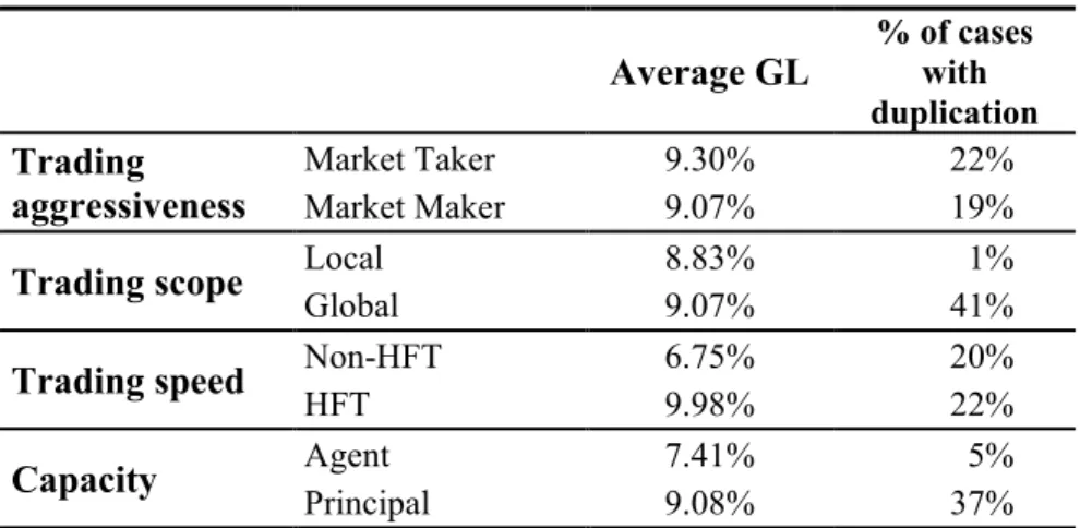
Finally, it is important to understand whether GL is mainly due to some categories of members. Table 5 decomposes average GL by members according to their trading scope (local trader and
global trader) and trading aggressiveness (market taker and market maker). We further distinguish
according to their trading speed (Non-HFT and HFT) and their capacity (Agent or Principal). The most interesting differences arise when comparing members acting as principal and those acting for their clients and when comparing HFTs and non-HFTs. As we would expect, the average GL for HFTs is larger than for non-HFTs and GL is typically higher when members are acting as principal rather than agent. Let us recall that the starting point of a GL calculation is a trade on a given venue. At the time of the trade, the passive counterpart may or may not have duplicated limit orders on the venue where GL is measured. For that reason, we also provide, in Table 5, the percentage of trades for which there is order duplication on the GL venue. By definition, this percentage is extremely low for local traders (1%), but in those seldom cases where they duplicate orders, the average value of their GL is similar to that of global traders. Another striking case is that of members trading as agent. They duplicate limit orders far less often than members trading as principal (5% vs. 37%), and when they do so, their level of GL is slightly lower.
The fact that on average GL differs across member categories suggests that it may be important to control for such categories in our multivariate analysis. We now turn to our empirical model and identification strategy.
6. Determinants of GL
In this section we study the empirical determinants of GL. Our left-hand side variable is the daily stock- and member-specific GL measure defined at Equation (2) and in our base model t = 10ms.
Our regression model is
. ; ; ; , , , , , 5 , 4 , 3 , 2 , 1 , , \ 2 , , \ 1 , 2 , 1 , , , 3 , 3 , 2 , 1 qv tv m d i d i d i d i d i d i Others m d i nonHFT Others m d i HFT qv tv qv tv m d i m i m i m i m i qv tv FRAG TICK PRICE VOLUME GL GL ALTtoPE PEtoALT TRADESIZE GLOBAL MM AGENT HFT m d i t GL (5)
t i d m
GLtvqv ; ; ; is the aggregated GL on venue qv resulting from a trade on venue tv, for
15
member characteristics. We further include trade, platform, other market member, and stock characteristics as well as different sets of fixed effects. Depending upon the model, the set of fixed effects include stock-fixed effects and/or day-fixed effects.
The market member characteristics consist of four dummy variables HFT, AGENT, MM, and
GLOBAL. They are equal to one when in that stock, a market member is an HFT, trading as agent,
market maker, or global trader respectively, and zero otherwise. As a trade characteristic we include TRADESIZE. The platform characteristics capture whether tv and qv are the primary exchange (PE) or one of the alternative venues (ALT). PEtoALT is one when trade venue tv is PE and the venue on which we measure GL (i.e., qv) is ALT, zero otherwise. ALTtoPE has a similar interpretation. The base case is where tv and qv are both ALT. We further control for the GL by other HFT members ( Others
m d i HFT
GL \, , ) and other non-HFT members ( Others m d i nonHFT
GL \, , ) excluding member
m (denoted by \m) on day d for stock i. Finally, we also include stock-day characteristics such as
the realized volatility (), the trading volume (VOLUME), the stock price (PRICE), the tick size (TICK) and the degree of fragmentation (FRAG). Realized volatility i,d is computed as the square root of the average squared five-minute logarithmic returns of stock i over day d.
d i
VOLUME , is the logarithm of the total euro volume traded in stock i on the four venues over day d. PRICEi,d is the last cross-venue midquote of day d for stock i, taken in logarithm. FRAGi,d
, the degree of fragmentation of stock i on day d, is the reciprocal of a Herfindhal-Hirschman index based on the market shares in volume of the four trading platforms.6
We employ a Tobit model as our dependent variable has truncations at zero and one, i.e., in many instances there is no withdrawal of liquidity, or all liquidity is withdrawn.
Table 6 about here
Table 6 displays the results for our empirical model employing different sets of fixed effects. Column (1) does not contain stock or day fixed effects. Columns (2) and (3) include day and stock fixed effects, respectively. Column (4) includes both day and stock fixed effects.
6 This type of measure is commonly used in the literature on market fragmentation (see Degryse et al. (2015) and
Gresse (2017)). In terms of interpretation, our FRAG index ranges from one to four, one indicating no fragmentation, or in other words, a consolidation of volumes on a single venue, and four indicating maximum fragmentation, that is volumes equally distributed across the four venues. A FRAG index of two would mean that the level of fragmentation is equivalent to the maximum level of fragmentation between two markets, i.e., 50% of the volumes on each.
16
We first examine the member characteristics – our key variables of interest. As results are qualitatively very similar across the (4) columns, we focus on column (4) that includes both day and stock fixed effects. HFTs lead to more GL than otherwise similar trades against non-HFTs. In particular, an HFT member withdraws 3.44*** percentage points more of its outstanding limit orders on venue qv following the execution of one of its limit orders on venue tv compared with a non-HFT member facing a similar situation. GL is also more pronounced when (i) a member is a market maker (0.89*** percentage points), (ii) a member is a global trader (12.4*** percentage points), and (iii) acts as principal (1.86*** percentage point, i.e., agent=0).
The next row investigates whether “trade characteristics” determine GL. GL is larger when the trade on trading venue tv is larger. Members have more incentives to cancel orders when trade size on the trading venue is larger. Column (4) shows that when trade size doubles, GL increases by 0.94** percent. Larger trades thus induce more GL.
The next rows in Table 6 show the results for the “platform characteristics”. Based on column (4), the PEtoALT coefficient shows that GL is 1.95*** percentage points less pronounced when the trade takes place on the primary exchange and the GL venue is another venue compared to the base case ALTtoALT. The coefficient on ALTtoPE is economically small and only significant when excluding stock-fixed effects. Put differently, it seems that GL is somewhat higher among the non-primary exchanges and from other venues to the non-primary exchange.
Our regression model controls for other members’ GL activity on that day for that stock. Based on column (4), GL by member m is 3.56*** and 6.61***percentage point larger when GL of other HFTs and non-HFTs increase by 100%, respectively.
Finally, we report the results on our stock characteristics. Across the various specifications with differing sets of fixed effects, the coefficients on trading volume and fragmentation are always significant and positive, implying that GL is greater for stocks that are traded more heavily and in a dispersed set of locations. Larger GL in times of greater volatility, lower price and higher relative tick size is found in some specifications, but the significance of these effects does not survive the inclusion of stock fixed effects.
All in all, our results reveal that members that are HFT, market makers, and are global exhibit a significantly higher GL than otherwise similar traders.
17 7. Conclusion
The objective of this paper is to assess the scale of Ghost Liquidity (GL) and the factors that drive it in fragmented markets. GL is related to limit order duplication across venues, with the intention of cancelling some of them immediately after one of them executes. Such liquidity provision strategies are built to maximize execution probabilities. On the one hand, they may benefit cross-market liquidity by improving execution probabilities, yet on the other hand, GL may mislead market participants in their perception of the true liquidity available in the marketplace. By drawing on a unique data set that covers the primary exchange and the three main alternative trading venues in Europe, i.e., Chi-X, BATS, and Turquoise, for 91 European stocks primary listed in nine countries, we find that, in the presence of duplicated limit orders, a substantial portion of the corresponding liquidity is GL: 9.12% on the primary exchange, 8.48% on Chi-X, and more than 7% on BATS and Turquoise. The level of GL differs across stocks and countries. Countries with the highest levels of GL are the Netherlands (13.88%) and France (10.38%), and countries with the lowest GL levels are Spain (3.75%), Italy (6.06%), and Portugal (6.21%). Across stocks, stocks pertaining to the tercile of the largest market values have the greatest GL while stocks with the lowest GL are those of the middle tercile. Further, GL increases with volatility, trading volume, and market fragmentation. Market participants who most contribute to GL are HFTs trading as principal and traders behaving as market makers on several trading venues.
18 References
Bouveret, Antoine, Guillaumie Cyrille, Aparicio Roqueiro, Carlos, Winkler, Christian, and Nauhaus, Steffen (2014). High-frequency trading activity in EU equity markets. ESMA Economic Report #2.
Brogaard, Jonathan (2010). High frequency trading and its impact on market quality. Northwestern University Kellogg School of Management Working Paper, 66.
Brogaard, Jonathan, Hendershott, Terrence J., and Riordan Ryan (2014). High-frequency trading and price discovery. Review of Financial Studies, 27(8), 2267-2306.
Carrion, Allen (2013). Very fast money: High-frequency trading on the NASDAQ. Journal of
Financial Markets, 16(4), 680-711.
Degryse, Hans, de Jong, Frank, and van Kervel, Vincent (2015). The impact of dark and visible fragmentation on market quality. Review of Finance, 19(4), 1587-1622.
Foucault, Thierry, and Menkveld, Albert (2008). Competition for order flow and smart order routing systems”, Journal of Finance, 63(1), 119-158.
Gresse, Carole (2017). Effects of lit and dark market fragmentation on liquidity. Journal of
Financial Markets, forthcoming.
Hasbrouck, Joël, and Saar, Gideon (2009). Technology and liquidity provision: The blurring of traditional definitions. Journal of financial Markets, 12(2), 143-172.
Hasbrouck, Joël, and Saar, Gideon (2013). Low-latency trading. Journal of Financial Markets, 16(4), 646-679.
Hendershott, Terrence J., Jones, Charles J., and Menkveld, Albert J. (2011). Does algorithmic trading improve liquidity?. Journal of Finance, 66(1), 1-33.
Jovanovic, Boyan and Menkveld, Albert J. (2016). Middlemen in limit order markets. Working Paper available at http://dx.doi.org/10.2139/ssrn.1624329.
Kirilenko, Andrei A., Kyle, Albert S., Samadi, Mehrdad, and Tuzun, Tugkan (2016). The flash crash: High frequency trading in an electronic market, Journal of Finance, forthcoming. Menkveld, Albert J. (2013). High frequency trading and the new market-makers”, Journal of
Financial Markets, 16(4), 712-740.
Menkveld, Albert J. (2016). The economics of high-frequency trading: Taking stock. Annual
19
O’Hara, Maureen, and Ye, Mao (2011). Is fragmentation harming market quality?”, Journal of
Financial Economics, 100(3), 459-474.
van Kervel, Vincent (2015). Competition for order flow with fast and slow traders. Review of
20 Table 1. Descriptive statistics on sampled stocks
Country Number of stocks Market value (EUR Mn) Value traded (EUR Mn) Cross-market bid-ask spread Market share of the primary exchange Belgium 6 Mean 24,327 2,012 0.0465% 72,13% Min. 843 86 0.0181% 62,44% Max. 118,942 8,134 0.0956% 88,78% France 15 Mean 7,957 1,632 0.0362,% 74,73% Min. 195 2 0.0063,% 62,35% Max. 55,979 12,658 0.1006,% 97,30% Germany 13 Mean 10,039 1,997 0.0962,% 74,80% Min. 242 10 0.0084,% 59,25% Max. 71,713 15,074 0.4480,% 95,63% Ireland 4 Mean 4,551 291 0.0450,% 86,20% Min. 1,599 46 0.0010,% 79,97% Max. 7,898 709 0.0951,% 93,07% Italy 11 Mean 6,495 1,454 0.0305,% 86,84% Min. 292 7 0.0015,% 79,01% Max. 27,628 6,234 0.1609,% 98,31% Portugal 4 Mean 6,035 944 0.0047,% 74,92% Min. 2,080 612 0.0010,% 63,14% Max. 10,857 1,090 0.0135,% 85,44% Spain 12 Mean 9,650 1,884 0.0098,% 85,02% Min. 801 299 0.0024,% 78,77% Max. 40,712 10,613 0.0238,% 92,35% The,Netherlands 11 Mean 7,747 1,771 0.0181,% 75,43% Min. 383 54 0.0014,% 64,80% Max. 50,233 9,036 0.0607,% 87,64% The,United,Kingdom 15 Mean 8,529 1,228 0.0189,% 65,27% Min. 395 16 0.0028,% 53,47% Max. 69,843 6,969 0.0480,% 79,80% Total 91 Mean 9,481 1,468 0.0340,% 77,26% Min. 195 2 0.0010,% 53,47% Max. 118,942 15,074 0.4480,% 98,31% This table reports the number of stocks sampled by country and, for each country, the average, the minimum, and the maximum values of the market value in million euros, the total traded value in May 2013 in million euros, the cross-market bid-ask spread, and the cross-market share of the primary exchange. Four cross-markets are considered: the primary exchange, Chi-X, Bats, and Turquoise.
21 Table 2. Member categories
Trading scope Trading aggressiveness Trading speed Capacity Number of member/stock combinations % in trading volume
Total exchange Primary BATS Chi-X Turquoise
Local trader Market taker Non-HFT A 3,259 15,80% 15,72% 0,01% 0,06% 0,01% P 1,241 4,88% 4,31% 0,02% 0,37% 0,18% HFT A 247 3,79% 3,78% 0,00% 0,01% 0,00% P 139 0,74% 0,50% 0,00% 0,19% 0,06% Market maker Non-HFT P 545 0,99% 0,81% 0,01% 0,10% 0,07% HFT P 183 0,98% 0,65% 0,02% 0,30% 0,02% Global trader Market taker Non-HFT A 527 3,23% 1,87% 0,24% 0,89% 0,22% P 817 20,22% 11,70% 1,13% 5,27% 2,12% HFT A 189 3,18% 1,82% 0,18% 0,63% 0,55% P 536 22,68% 12,53% 1,36% 5,69% 3,11% Market maker Non-HFT P 441 9,69% 5,73% 0,57% 2,42% 0,98% HFT P 444 13,81% 4,93% 1,40% 4,98% 2,49% Total 8,568 100% 64,35% 4,92% 20,91% 9,82%
This table displays the relative market size of each member category. Our member classification is established on a stock-by-stock basis and based on three criteria: local vs. global traders, market makers vs. market takers, and HFTs vs. non-HFTs. Flags for a given member on a given stock can also differ according to the member capacity (agent or principal). As a result, column “Number of member/stock combinations” displays numbers of member×capacity×stock combinations. The right-hand side of the table reports the percentages of each category in total trading volumes with a breakdown by exchanges.
22 Table 3. Average level of GL Panel A - By country
Belgium 9.79%
Germany 6.85%
Spain 3.75%
France 10.38%
The United Kingdom 8.71%
Ireland 9.17% Italy 6.06% The Netherlands 13.88% Portugal 6.21% Panel B - By platform Primary exchange 9.12% Chi-X 8.48% Turquoise 7.13% BATS 7.82%
Panel C - By pair of platforms
GL venue Trade venue
Primary exchange Chi-X 9.11%
BATS 8.70%
Turquoise 9.81%
Chi-X Primary exchange 8.61%
BATS 8.41%
Turquoise 8.08%
BATS Primary exchange 7.15%
Chi-X 8.12%
Turquoise 9.84%
Turquoise Primary exchange 6.90%
Chi-X 6.40%
BATS 7.40%
This table reports statistics on GL by country (Panel A), platform (Panel B), and pair of platforms (Panel C). GL is first estimated for each stock over the whole month of May 2013. Then, in each case, a cross-sectional equally-weighted mean is calculated. Those means reflect how much depth is cancelled by a given member on a given platform immediately after being executed on liquidity posted on another venue.
23
Table 4. Average level of GL per market value tercile Market value tercile Market value range
(EUR Mn) Average GL
1 195 to 1,833 9.32%
2 1,989 to 5,846 7.48%
3 6,152 to 118,942 8.26%
This table reports statistics on GL by market value tercile. GL is first estimated for each stock over the whole month of May 2013. Then, in each market size tercile, a cross-sectional equally-weighted mean is calculated. Those means reflect how much depth is cancelled by a given member on a given platform immediately after being executed on liquidity posted on another venue.
24
Table 5. Average GL by member category
Average GL % of cases with duplication Trading
aggressiveness
Market Taker 9.30% 22%
Market Maker 9.07% 19%
Trading scope Local 8.83% 1%
Global 9.07% 41%
Trading speed Non-HFT 6.75% 20%
HFT 9.98% 22%
Capacity Agent 7.41% 5%
Principal 9.08% 37%
This table reports statistics on GL by member category. GL is first estimated by stock and by member×capacity combination over the whole month of May 2013. Then, for each member category, a cross-sectional equally-weighted mean is calculated. Those means reflect how much depth is cancelled by a given member on a given platform immediately after being executed on liquidity posted on another venue. The last column reports the percentage of trades for which depth was actually duplicated before trading.
25 Table 6. Tobit regressions of GL
(1) (2) (3) (4) Member characteristics HFT 0.0332*** 0.0332*** 0.0344*** 0.0344*** Agent -0.0200*** -0.0199*** -0.0186*** -0.0186*** Market maker 0.0082*** 0.0082*** 0.0089*** 0.0089*** Global 0.1268*** 0.1268*** 0.1240*** 0.1240*** Trade characteristics Trade size 0.0089*** 0.0090*** 0.0093*** 0.0094*** Platform characteristics PE-to-alternative -0.0170*** -0.0170*** -0.0195*** -0.0195*** Alternative-to-PE 0.0005 0.0004 0.0016*** 0.0016***
Other market member GL
GL(others, HFT) 0.0537*** 0.0543*** 0.0355*** 0.0356*** GL(others, nonHFT) 0.0925*** 0.0926*** 0.0665*** 0.0661*** Stock characteristics Realized volatility 1.5560*** 1.6488*** -0.7582 0.1100 Volume 0.0066*** 0.0065*** 0.0106*** 0.0098*** Price -0.0032*** -0.0033*** 0.0113 0.0067 Tick 4.7879*** 4.6953*** -0.8673 -1.5480 Fragmentation 0.0180*** 0.0186*** 0.0066*** 0.0071*** Fixed effects
stock fixed effects NO NO YES YES
day fixed effects NO YES NO YES
Pseudo R² 21.28% 21.32% 22.19% 22.21%
This table reports the conditional marginal effects of Tobit regressions of daily measures of GL by member, stock, and pair of platform. Each pair of platforms consist of the trade venue, i.e., the venue where the member was passively executed, and the GL venue, i.e., the venue where the member liquidity is potentially withdrawn. Reported coefficients are the marginal effects on the positive observations of GL. The regressors include a measure of daily realized volatility, the total daily traded volume in logarithm, the closing price in logarithm, the relative tick size, the GL measured for other HFT members, the GL measured for other non-HFT members, a fragmentation index, the average size of the trades triggering the cancellation of GL, a HFT dummy equal to one for HFT members, an agent dummy equal to one for member trading as agent, a market-maker dummy equal to one for members identified as liquidity providers, a global dummy equal to one for cross-market members, a PE-to-MTF dummy equal to one when the trade venue is the primary exchange and the GL venue a MTF, and a PE-to-MTF dummy equal to one when the trade venue is the primary exchange and the GL venue a MTF. Tobit regressions are double-censored with a lower bound set to 0 and an upper bound set to 1. ***, **, * indicate statistical significance at the 1%, 5%, and 10% level respectively.