Science Arts & Métiers (SAM)
is an open access repository that collects the work of Arts et Métiers Institute of Technology researchers and makes it freely available over the web where possible.
This is an author-deposited version published in: https://sam.ensam.eu Handle ID: .http://hdl.handle.net/10985/9899
To cite this version :
Julien ARTOZOUL, Christophe LESCALIER, Daniel DUDZINSKI - Experimental and analytical combined thermal approach for local tribological understanding in metal cutting - Applied Thermal Engineering - Vol. 89, p.394–404 - 2015
EXPERIMENTAL AND ANALYTICAL COMBINED THERMAL APPROACH
FOR LOCAL TRIBOLOGICAL UNDERSTANDING IN METAL CUTTING
Julien Artozoul1,2, Christophe Lescalier1, Daniel Dudzinski2 Laboratoire d’Etudes des Microstructures et de Mécanique des Matériaux LEM3 - UMR CNRS 7239 - 4 rue Augustin Fresnel - 57070 Metz – France
(1) Arts et Métiers ParisTech (2) Université de Lorraine
Corresponding author : Daniel Dudzinski Phone number: (33) 3 87 37 42 86
E-mail address : [email protected]
Abstract
Metal cutting is a highly complex thermo-mechanical process. The knowledge of temperature in the chip forming zone is essential to understand it. Conventional experimental methods such as thermocouples only provide global information which is incompatible with the high stress and temperature gradients met in the chip forming zone. Field measurements are essential to understand the localized thermo-mechanical problem. An experimental protocol has been developed using advanced infrared imaging in order to measure temperature distribution in both the tool and the chip during an orthogonal or oblique cutting operation. It also provides several information on the chip formation process such as some geometrical characteristics (tool-chip contact length, chip thickness, primary shear angle) and thermo-mechanical information (heat flux dissipated in deformation zone, local interface heat partition ratio). A study is carried out on the effects of cutting conditions i.e. cutting speed, feed and depth of cut on the temperature distribution along the contact zone for an elementary operation. An analytical thermal model has been developed to process experimental data and access more information i.e. local stress or heat flux distribution.
Keywords:
tool-chip interface, temperature, infrared thermography, orthogonal cutting, analytical model, inverse method
1. INTRODUCTION
Temperature and heat generation in metal cutting have been intensively studied in the past. Measurement techniques as well as modeling have been and are still developed. Temperature has a major influence on machining performance such as tool life as well as workpiece surface integrity
and then machined parts resistance. Bacci da Silva and Wallbank [1] and Abukhshim et al. [2] review critically the main previous works focused on the development of experimental, analytical and numerical approaches devoted to the thermal problem of metal cutting.
Analytical models are extensively reviewed by Komanduri and Hou, [3][4]; the main comments related to the analytical works are given in the following. These models are usually based on simplifying assumptions; they generally focus on a two-dimensional and steady state orthogonal cutting operation with simplified tool geometry. The cutting edge is assumed to be perfectly sharp and the rake face is flat. Tool or chip or workpiece are regarded as semi-infinite or infinite media. The material on each side of the primary shear zone is often supposed as two separate bodies in sliding contact; only few works assume it as the same body, [3] [5]. Both primary shear zone and secondary shear zone are considered as planes; tool-chip and tool-workpiece contact zones are currently supposed thermally perfect. Courbon et al. [6] propose an original approach for the tool-chip interface; this one is thermally perfect only for the sticking part of the contact zone whereas a thermal contact resistance is introduced for the sliding part. Generally the plastic deformation in the chip is neglected and the chip is supposed to move as a rigid body. Both tool and chip and workpiece free surfaces are generally regarded as adiabatic or rarely as convective heat transfer. Temperature distributions are currently predicted using Jaeger moving heat sources model [7].
The complete thermo-mechanical problem of cutting can be solved using finite element method. This numerical approach includes large deformation formulation; requires relevant friction laws and thermo-viscoplastic material behavior relations available at high strain rate and high temperature, [2]. The obtained models have to solve the tool-chip contact, and to manage the generation of a new surface by considering a separation criterion. As pointed out by Filice et al. [8] and Umbrello et al. [9], a large number of elements are necessary with refinement and remeshing processes to achieve an accurate description of local variables such as deformation and temperature; and due to the calculation time only a limited cutting length may be simulated; thus the steady-state may not be easily reached.
However, with the assumption of a single sliding zone at the tool-chip interface, the proposed model overestimates the interface temperatures. Bahi et al. [12] introduce a more complex friction law considering both sticking and sliding contacts and propose a pioneering hybrid analytical-numerical approach. Karpat et al. [13] or Li et al. [14] finally implement the tertiary shear zone i.e. the tool-workpiece contact zone.
This paper proposes an analytical model to determine the temperature distribution in the tool and the work material during an orthogonal cutting process. The assumptions are very similar to those proposed by Komanduri and Hou [3], [4] and [15]. In addition, a parametric model is proposed for the heat source representing the secondary shear zone; it considers both sticking and sliding regions. Temperature distribution is then predicted in the whole cutting zone. Moreover orthogonal cutting experiments are performed; transient temperature distributions are collected using infrared thermography technique. In cuttingprocess, the tool-chip interface is the most critical zone with high stresses and high temperatures values; results are focused on this area. Predicted and measured temperatures at tool-chip interface are thus correlated to provide some significant information about heat flux and heat partition ratio, the normal and shear stresses distributions are extracted then and discussed.
2. EXPERIMENTAL PROCEDURE
Orthogonal cutting tests were carried with a Sandvik Coromant turning tool using a TPUN 160308 GC235 coated carbide insert and a CTFPR 2525 M16 tool holder. Rake angle and relief angle are respectively equal to 6° and 5°. The tested cutting conditions are given in Table 1.
Cutting speed VC (m/min) 50 100 150 250 Feed f or undeformed chip thickness t1 (mm/rev) 0.3
Width of cut w (mm) 2
Table 1 - Cutting conditions
The work material was an AISI 1055 medium carbon steel. It is provided as 50 mm diameter hot rolled rods. Table 2 summarizes its main mechanical characteristics.
Yield stress (MPa) Tensile strength (MPa) Hardness HV30
370 700 200
Table 2 – Work material mechanical characteristics
Cutting forces were measured using a dynamometric table Kistler 9257A. Temperature distributions were measured using a FLIR SC7000 camera equipped with a G3 lens. The spatial resolution of the
images provided is about 15 µm x 15 µm per pixel. Further information should be found in Artozoul et al. [16]. Analytical calculations are based on assumed thermo physical values for both steel and carbide given in Table 3.
AISI 1055 Tool
Symbol Value Symbol Value Density (kg/m3)
w 7,850 tool 11,100
Thermal conductivity (W/m.K) w 55 tool 37.7
Heat capacity (J/kg.K) cw 460 ctool 276
Table 3 – Material thermo physical properties
3. MODELING AND INVERSE APPROACH
For an orthogonal cutting process, the tool cutting edge is parallel to the work surface and normal to the cutting direction. The feed f or undeformed chip thickness t1 is small compared to the width of cut w, and then the chip is formed under approximately plane strain conditions. The tool is perfectly
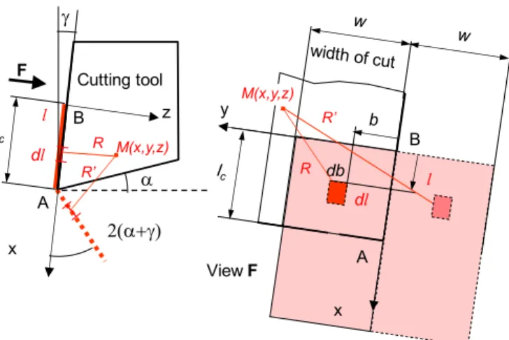
sharp and assumed to be a rigid body; its width is larger than the width of cut w. The chip is formed by shearing in a narrow zone, the so-called Primary Shear Zone (i.e. PSZ). PSZ is reduced to a plane, of length L, according to the Merchant theory [17]; and its inclination in relation to the cutting direction is defined by the shear angle . Beyond this Primary Shear Zone, the chip is sliding on the tool rake face and is deformed in a Secondary Shear Zone (i.e. SSZ). This zone is assumed to be a plane of length lc, the tool-chip contact length, and width w, the width of cut. The two main heat sources are these two shear zones, Figure 1; they are due to plastic deformation and additionally to friction in the SSZ zone. The Tertiary Shear Zone at tool-workpiece contact is ignored.
width of cut
w
Adiabatic boundaries
Chip Velocity VChip
Cutting tool Cutting tool
to PSZ and SSZ. The tool-chip contact is regarded as thermally perfect. A local heat partition ratio is introduced and values are calculated along the tool-chip contact zone to meet this assumption. All the free surfaces are considered as adiabatic boundaries which is acceptable assumption when dry cutting.
3.1 - Primary shear zone
Following Komanduri and Hou [3], the shear plane can be considered as a band heat source moving continuously and obliquely in the surface layer of the workpiece (the layer under the workpiece free surface of thickness t1 equal to the feed f ) with the cutting velocity VC, see Figure 2a. In the same
way, the shear heat band is assumed to be moving continuously and obliquely in the chip with the chip flow velocity VChip , see Figure 2b.
The workpiece and the chip are assumed to be semi-infinite bodies. The frame (X,z) is always associated to the heat source; the X-axis is along the heat source velocity direction. The heat velocity
V is the velocity relative to the workpiece (V =VC ), Figure 2a, or to the chip (V =VChip ), Figure 2b.
(a) (b)
Figure 2 - Primary Shear Zone PSZ assumed to be a band heat source moving continuously and obliquely
(a) in the workpiece with the cutting velocity VC , and (b) in the chip with the chip flow velocity VChip,. The length of the PSZ in the (z,X) is L. The coordinate system (X,Y,Z) is associated to the moving source. Surfaces aOe, for the workpiece, and bOg for the chip are assumed to be adiabatic. The method of image sources will help in working out temperature distribution as described in appendix. In Figure 2, the image sources are represented with dashed lines. Increase in temperature in the workpiece and in the chip is worked out using formula (A-11) for a heat source moving obliquely in a semi-infinite medium with an adiabatic boundary surface, they are given by the following expressions:
f VC X z 2 f t1= f O a e R’ dl l M(X,z) R X z
f t2 VChip O g f R R’ M(X,z) dl b l
sin 2 0 0 0,
'
2
2
2
C w L X l V a workpiece PSZ C C PSZ w w wq
V
V
T
X z
e
K
R
K
R
dl
a
a
(1)
sin 0 0 2 02
2
'
,
2
w chip X l chip chip chip PSZ w w L V a PSZ wV
V
q
K
R
K
R
a
a
T
X z
e
dl
(2)With
R
X l
sin
2
z l
cos
2 andR
'
X l
sin
2
z l
cos
2which R and R' are respectively the distances of a point M(X,z) of the workpiece (or of the chip) from an element dlof the band heat source and of the its corresponding image, figure 2. a is the thermal w
diffusivity of the workpiece; qPSZ is the heat flux generated in the primary shear zone and flowing into both the chip and the workpiece. It can be calculated using the following formula:
1
sin
S S S S PSZV F
V F
q
wL
w t
f
(3)It is assumed that all shear energy is converted into heat. V and S F are respectively the shear velocity S
and the shear force component:
cos cos S C V
Vf
FS FCcosfFFsinf (4) CF and F are the measured cutting and feed force components, F
f
is the shear angle determined experimentally, see Figure 3. The temperature distributions on the imaginary sides are not valid and hence are not taken into consideration.It must be noted that in this approach no heat partition coefficient is necessary and that a single body is considered to model the material in each side of the primary shearing zone. The temperature distributions below and beyond the shear band are determined with the same heat flux qPSZ.
Figure 3 - Cutting forces and hodograph for orthogonal cutting.
3.2 Secondary shear zone
3.2.1 Increase in temperature
For the chip
As previously mentioned, the Secondary Shear Zone (SSZ) may be considered as a band heat source moving obliquely ( with
2) along the tool-chip interface, with a velocity equal to the chip velocity VChip, see Figure 4. The chip is assumed to be a semi-infinite medium (X>0), with anadiabatic boundary surface at z t . Once more, an image heat source is added; it is located at a 2 distance of 2t2 from the tool-chip interface.
The increase of temperature at a point M(X,z) of the chip due to the SSZ is then determined using the expression (A-10). Following here Trigger and Chao [18], it is multiplied by two to consider the case of a semi-infinite medium. It is then integrated along the contact zone (for l = 0 to lC), and finally an
image heat source is introduced due to the adiabatic surface boundary:
2 0 0 01
,
'
2
2
lC VChip X l aw Chip Chipchip chip SSZ SSZ W w w
V
V
T
X z
q
e
K
R
K
R
dl
a
a
(5) WithR
X l
2
z
2 andR
'
X l
2
2
t
2
z
2 . chip SSZq is the heat flux due to the secondary shear and frictional zone and transmitted to the chip; it is a fraction of the heat flux qSSZemitted at the secondary shear and frictional zone, defined in the following. Chip Cutting tool f f FC FF R FS NS f VChip VC VS Shear velocity FN R’ FT
Figure 4 - Secondary shear zone SSZ. The chip is assumed to be a semi-infinite medium X>0, with an adiabatic
boundary surface z t 2. The heat source is a band moving along the tool-chip interface.
For the tool
The tool is considered as a semi-infinite medium z>0 and the secondary shear and frictional zone at the tool-chip interface is assumed to be a rectangular heat source. The length of the heat source corresponds to the tool-chip contact length lc and its width w is equal to the width of cut, Figure 5. In appendix, the solution for a continuous point heat source is presented, formula (A-5). It may be used for an elementary surface
dl db
of the SSZ and increased twofold to get the elementary rise in temperature for the semi-infinite medium z>0:2 tool tool SSZ SSZ tool q dl db dT R (6)
To take into account of the adiabatic tool clearance face, an image source is added. It is represented by the dashed line in Figure 5. The elementary rise in temperature of the tool is thus given by:
1
1
2
'
tool tool SSZ SSZ toolq
dT
dl db
R R
(7) lc VChip t2 t2 z X A B R’ dl l R M(X,z)Figure 5 - Secondary shear zone SSZ. The tool is considered as a semi-infinite medium z >0, the clearance
face is assumed adiabatic. The frame Bxyz is linked to the fixed heat source with respect to the tool.
The temperature rise at a point M x y z
, ,
of the tool is calculated by integrating the previous expression along the contact length (from l 0 to l ) and along the width equal to twice the lCwidth of cut (or for b w to b w) to consider a semi-infinite medium y>0 :
, ,
1 0 1 1 2 ' C l w tool tool SSZ w SSZ tool T x y z q dl db R R
(8) withR
x l
2
y b
2
z
2and
R
'
x l
C
l
C
l
cos 2
2
y b
2
z
l
C
l
sin 2
2tool SSZ
q is the heat flux due to the secondary shear and frictional zone and transmitted to the tool. In the following, this heat flux is considered as a function of the coordinate x.
3.2.2 Heat partition
It must be noted that
q
SSZtool corresponds to a fraction
1BSSZ
of local heat fluxq
SSZ produced atthe secondary shear and frictional zone evacuated by the tool, while the fraction BSSZis transferred into the chip:
; 1 chip tool SSZ SSZ SSZ SSZ SSZ SSZ q B q q B q (9)At tool-chip interface, where the velocity is VChipand the tangential force (also called friction force) is T
F , it is assumed that all the power VChip FT is converted into heat; thus per unit surface the mean heat flux is calculated using :
0 0 c l w SSZ Chip T q dl dw V F
(10) F z x 2 View F A B A B y x l b db dl M(x,y,z) R’ R M(x,y,z) R R’ dl lwith
sin
cos C Chip V Vf
f
and
FT FCsinFFcos according to Figure 3. (11) Heat flux is assumed to be uniformly distributed along the width-direction of tool-chip interface and variable along the direction of its length:
0 c l SSZ Chip T w q
l dl V F (12)with
qSSZ
l l c
0 (13)A mathematical expression for heat flux is proposed in the following, it describes the sticking and sliding contact involving in the tool-chip interface:
1 ( ) when 0 0,1 SSZ c q l q l k l and k (14) ( ) 2 ( ) ( n l lc 1) when 0 SSZ c c q l q e k l l l and n (15)Along the sticking zone the heat flux is assumed to be constant; this assumption is coherent with the fact that in this zone the shear stress is usually considered as constant. In the sliding zone, heat flux is assumed to decrease exponentially.
The boundary condition (13) is verified by the expression (14); thus the constants q1 and q2 may be found by using relation (12) and the continuity of heat flux qSSZ at the junction of the two zones (sticking and sliding zones). Only two coefficients have to be introduced: the constant k which defines the decomposition of the tool-chip contact length into sticking contact and sliding contact; and the coefficient n which characterizes heat flux decreasing in the sliding zone.
Equations (14) and (15) are able to describe a large range of distributions: uniform heat flux distribution when k = 1 (full sticking zone), or exponential one when k = 0 (full sliding zone), and various others between these two particular cases.
To illustrate the previous propositions, Figure 6 and Figure 7 present examples of calculation for the distributions of heat flux and of heat partition ratio BSSZ at the secondary shear zone, for three sets of
k and n parameters (k=0.1 n=3,000, k=0.3 n = 1,000, k=0.8 n = 300). It must be noted that the ratio
SSZ
B corresponds to the fraction of heat transmitted to the chip and it regularly decreases from the cutting edge to the end of the tool-chip contact.
Figure 6 – Examples of heat flux distributions along the tool-chip contact for
three values of k defining the repartition between sticking and sliding zones and three values of n characterizing the decreasing of heat flux in the sliding zone.
Figure 7 – Examples of distribution of the heat partition ratio BSSZ, along the tool-chip contact for various values of k and n.
Using the equations (5) and (8), the temperature rise at the tool-chip interface is determined for the three sets of coefficients k and n values and the corresponding distribution at the tool-chip interface are presented in Figure 7. It is interesting to note that the maximum temperature always appears in
0 400 800 1,200 1,600 2,000 0.00 0.20 0.40 0.60 0.80 1.00 H ea t flu x (W/ mm² )
position on tool-chip contact length (0 cutting edge - 1 end of tool-chip contact length)
k = 0.1 n = 3,000 k = 0.3 n = 1,000 k = 0.8 n = 300 0.60 0.80 1.00 1.20 1.40 1.60 0.00 0.20 0.40 0.60 0.80 1.00 H ea t p a rtiti o n r a tio BSSZ (l )
position on tool-chip contact length (0 cutting edge - 1 end of tool-chip contact length)
k = 0.1 n = 3,000 k = 0.3 n = 1,000 k = 0.8 n = 300
the sliding zone, just after the boundary between sticking and sliding area. With the experimental determination of the temperature repartition at the tool-chip interface and by using the presented modeling, it will be now possible to have an idea of the contact conditions at the tool-chip interface and more precisely to know the decomposition of this zone between sticking and sliding.
Figure 8 – Resulting temperature distributions along the tool-chip interface
for the three sets of k and n values.
The model equalizes temperatures on the both sides of the tool-chip interface and implicitly assumes a perfect thermal contact. Moreover it proposes a local heat partition ratio between tool and chip; and, the heat flux varies all along the tool-chip interface depending on the contact conditions.
3.3 Superposition
From the previous modeling, the temperature at any point M x y z
, ,
of the tool is, in a first step, obtained with the temperature rise tool
, ,
SSZ
T x y z
, Equation (8), due to the secondary shear zone:
, ,
0
, ,
tool
tool SSZ
T x y z T T x y z (17)
the temperature at any point M X z
,
of the workpiece is determined with the temperature rise 0 200 400 600 800 1,000 0.00 0.20 0.40 0.60 0.80 1.00 Te mp e ra tu re ( °C)position on tool-chip contact length
(0 cutting edge - 100% end of tool-chip contact length)
k = 0.1 n = 3,000 k = 0.3 n = 1,000 k = 0.8 n = 300
,
0
,
,
Chip Chip
Chip PSZ SSZ
T X z T T X z T X z (19)
In this first step of calculation, the influence of the secondary shear zone SSZ in the workpiece and of primary shear zone PSZ in the tool are not considered. The cutting speed is high enough to neglect heat conduction in the opposite direction to the cutting speed, due the secondary shear zone. On the contrary, the influence of PSZ in the tool has to be taken into account, and a fictitious heat source distribution qtoolPSZ is added at the tool-chip interface. This heat flux distribution qtoolPSZ is determined in such a way to obtain, at the tool-chip interface, the same temperature rise, due to the primary shear zone, in the chip and in the tool. The rise in temperature in the chip is calculated with Equation (2); and, the temperature rise in the tool is determined with Equation (8), where the heat flux qSSZtoolis replaced by the fictitious heat flux qPSZtool:
, ,
1 0 1 1 2 '
lC w tool tool PSZ w PSZ tool T x y z q dl db R R
(20)Finally, the temperature at any point of the tool, due to heat generation in both primary and secondary shear zones, is given by:
, ,
0
, ,
, ,
tool tool
tool SSZ PSZ
T x y z T T x y z T x y z (21)
It is now possible to combine the experimental and the modeling approaches to obtain information about the contact conditions at the tool-chip interface and to predict the temperature fields in the tool, the chip and the workpiece.
4. RESULTS AND DISCUSSION
Cutting forces are measured using a Kistler dynamometric table. Experimental values are given in the Table 4. Analysis of images provided by the IR camera provides chip thickness and then actual chip velocity Vchip based on mass flow conservation (see Equation (10)).
Cutting speed VC
(m/min) Chip velocity Vchip (m/min) Cutting force F(N) C Feed force F(N) F 50 100 150 250 40±5 85±15 125±25 220±35 1,300±40 1,190±60 1,150±80 1,090±50 640±30 480±40 430±70 380±70
A post-processing technique has been developed to locate, with accuracy and objectivity, the cutting tool contour on the camera recordings and then provide relevant estimation of shear angle f and tool chip contact length lc. Shear angle values are extracted for each cutting test repeated twice, and a
mean value and standard deviation are calculated.
is the friction angle determined from the experimental cutting and feed forces results through:
tan
tan
tan
C F T N C FF
F
F
F
F
F
(22)where is the apparent friction coefficient, and the rake angle.
Figure 9 gives all the experimental results: the cutting and feed forces F and C F measured with the F
dynamometric table; the evolution of the apparent friction angle µ calculated with relation (22); the shear angle f and the tool-chip contact length lc obtained from the camera recordings.
0 300 600 900 1,200 1,500 0 60 120 180 240 300 FC (N ) -FF (N )
cutting speed Vc (m/min)
Fc (N) Ff (N) 0.0 0.2 0.4 0.6 0.8 1.0 0 60 120 180 240 300 A p p ar e n t fr ic tion c oe ff ic ie n t µ
cutting speed Vc (m/min)
35 40 45 50 55 Sh e ar a n gle f (° ) 0.3 0.6 0.9 1.2 1.5 l c h ip c on ta ct l e n gt h lc ( mm )
Figure 10 - Temperature computed and measured with IR Camera,
for the three tested values of cutting speed and for a feed f=0.3 mm/rev.
Using temperature fields and tool-chip contact length experimental value, it is then possible to extract the temperature distribution along the tool-chip interface. Figure 10 gives the distribution for the three tested cutting speed values. The following operation consists in applying the thermal model to obtain a probable heat flux distribution by inverse model fitting. The coefficients k and n, introduced in equations (14) and (15), are adjusted to fit experimental temperature distributions with the model ones. This operation is done for all the cutting conditions and leads to estimated heat flux distributions, Figure 11. They correspond to k = 0 (total sliding zone), and a value of n of about 3200 m-1, for the three cutting tested conditions. As no sticking zone is found at the tool-chip interface, the chip is assumed to slide on the rake face with an uniform velocity Vchip ; and, from the knowledge of local heat flux qSSZ it is then possible to determine the shear stress from :
cos
sin
SSZ SSZ Chip Cq
q
V
V
f
f
(23)Based on the qSSZ distribution, it is then possible to process the shear stress distribution at the tool-chip interface. As it can be seen, Figure 11, the shear stress at the tool-tool-chip interface is maximal on the cutting edge and is decreasing to 0 at the end of the contact length. The obtained shear stress levels for the two lower cutting speeds (i.e. 50 and 150 m/min) appear very close and is much higher for the cutting speed of 250 m/min. It is interesting to note that using this method; it was possible to get information about stress distribution, which is usually very difficult to obtain by direct measurement. 200 300 400 500 600 700 0.00 0.20 0.40 0.60 0.80 1.00 Te mp er at u re ( °C)
position on tool-chip contact length (0 cutting edge - 1 end of tool-chip contact length)
Vc = 250 m/min Vc = 100 m/min Vc = 50 m/min
Figure 11 - Heat flux and shear stress distribution,
for the three tested values of cutting speed and for a feed f=0.3 mm/rev.
It has been pointed out that temperature fields in metal cutting can be properly measured using infrared thermography [1][2][19]; but the measurements are relevant only for the tool, because the tool is immobile relatively to the camera while the work material continuously flows. In the other hand, thermal modeling provides information on the full cutting area as well in the tool, the chip or even the workpiece. In Figure 12, only chip and tool temperature fields, due to primary and secondary shear zones, are plotted in order to compare them with experimental results (see Figure 10). As the cutting speed increases, temperature rise in the chip, due to secondary shear zones, appears more confined at the vicinity of the tool chip contact zone.
(a) (b) (c)
f =0.3 mm/rev ,
(a) Vc = 50, (b) Vc = 100 and (c) Vc = 250 m/min
Figure 12 - Temperature fields computed from modeling in both tool and chip.
0 750 1500 2250 3000 0.00 0.20 0.40 0.60 0.80 1.00 H ea t fl u x d en si ty qSSZ (W/ mm² )
position on tool-chip contact length (0 cutting edge - 1 end of tool-chip contact length)
Vc = 50 m/min Vc = 100 m/min Vc = 150 m/min Vc = 250 m/min 0 300 600 900 1200 0.00 0.20 0.40 0.60 0.80 1.00 Sh ea r st re ss (N/ mm² )
position on tool-chip contact length (0 cutting edge - 1 end of tool-chip contact length)
Vc = 50 m/min Vc = 100 m/min Vc = 150 m/min Vc = 250 m/min
cutting conditions. Values are pretty close despite the change in cutting conditions. Mean value and standard deviation are then computed. It tends to increase with regards to cutting speed. However values remain lower than 5 W/mm². A ratio of fictitious heat flux to secondary shear zone heat flux is also computed. The correction due to the primary shear zone remains negligible since ratio is systematically lower than 5%.
(a) (b)
Figure 13 – Typical fictitious heat source distribution – Evolution with regards to cutting speed
BSSZ values are computed in an unconstrained way for the whole cutting conditions (see Table 1). It means that BSSZ can take values outside the range [0, 1]; negative values as well as values greater than 1 could then appear. A value greater than 1 (see Figure 14-a) is currently related to heat sinks on the tool side; it is commonly seen in the vicinity of the cutting edge [18]. Once more BSSZ values are very close despite the changes in cutting conditions since cutting speed varies from 50 to 250 m/min. It is hard to get an overview of the heat partitioning trend based on BSSZ distributions. It may be easier to get it through
B
or mean value of BSSZ.B
is used to equalize the two mean temperatures at the tool-chip interface : the one computed on tool side and the other computed on chip side. Similar approach is proposed by Shaw [20] but with more basic assumptions about secondary shear zone heat rate.B
is then computed according to Shaw [20] in order to compare trends and values.BSSZ depends on the distance to the cutting edge. Numerical values of BSSZ are rather different along the tool-chip interface: from 0.7 to 1.4 for the lower cutting speed. A mean value of BSSZ is computed and compared to the different values of
B
. Trends as well as values are pretty similar: heat partition ratio tends to increase with the cutting speed regardless the criterion.0 3 6 9 12 15 0.00 0.20 0.40 0.60 0.80 1.00 qPSZ to o l(W/ mm² )
position on tool-chip contact length (0 cutting edge - 1 end of tool-chip contact length)
0% 2% 4% 6% 8% 10% 0.00 1.50 3.00 4.50 6.00 7.50 0 60 120 180 240 300 ra tio o f S qPSZ to o lto S qSSZ Mea n v al u e o f qPSZ to o l (W/ mm² )
cutting speed Vc (m/min)
(a) (b)
Figure 14 – Heat partition ratio distribution – Evolution with regards to cutting speed
5. CONCLUSIONS AND PERSEPECTIVES
This paper proposes an analytical thermal model of metal cutting based on the initial approach of Komanduri and Hou [3][4][15]. It follows the experimental work of Artozoul et al. [16]. Both modeling and experimental approaches are combined to analyze the thermo-mechanical aspects of the tool-chip contact.
The main results can be summarized as follows:
1. From the thermal images of the cutting zone recorded for different integration times and for various cutting speed values, it is possible to determine shear angle, tool-chip contact length as well as chip velocity. Temperature fields in the tool and then temperature distribution at the tool-chip interface are extracted.
2. From the measured temperature at the tool-chip interface, and from the experimental cutting forces, it is possible through inverse analysis to identify both heat flux distribution and heat partition ratio between tool and chip. Results agree with previous literature results.
3. The global heat partition ratio at the tool-chip interface can be processed from experimental data and compared with theoretical values processed from previous research works. Values
0.20 0.60 1.00 1.40 1.80 0.00 0.20 0.40 0.60 0.80 1.00 BSSZ (l )
position on tool-chip contact length (0 cutting edge - 1 end of tool-chip contact length)
Vc = 50 m/min Vc = 100 m/min Vc = 150 m/min Vc = 250 m/min 0.80 0.85 0.90 0.95 1.00 0 60 120 180 240 300 H e at p ar tition r at io for SS Z
6. REFERENCES
[1] M. Bacci da Silva, J. Wallbank, Cutting temperature: prediction and measurement methods—a review. Journal of Materials Processing Technology, 88(1-3) (1999) 195‑202.
[2] N.A. Abukhshim, P.T. Mativenga, M.A. Sheikh, Heat generation and temperature prediction in metal cutting: A review and implications for high speed machining, International Journal of Machine Tools and Manufacture 46(7-8) (2006) 782-800.
[3] R. Komanduri, Z.B. Hou, Thermal modeling of the metal cutting process -- Part I: Temperature rise distribution due to shear plane heat source. International Journal of Mechanical Sciences 42(9) (2000) 1715-1752.
[4] R. Komanduri, Z.B. Hou, Thermal modeling of the metal cutting process -- Part II: temperature rise distribution due to frictional heat source at the tool-chip interface. International Journal of Mechanical Sciences 43(1) (2001) 57-88.
[5] R.S. Hahn, On the temperature developed at the shear plane in the metal cutting process, Proceedings of First U.S. National Congress of Applied Mechanics, (1951) 661–666.
[6] C. Courbon, T. Mabrouki, J. Rech, D. Mazuyer, E. D’Eramo, On the existence of a thermal contact resistance at the tool-chip interface in dry cutting of AISI 1045: Formation mechanisms and influence on the cutting process, Applied Thermal Engineering , 50(1) (2013) 1311–1325
[7] J.C. Jaeger, Moving sources of heat and the temperature at sliding contacts, Proceedings Royal Society of NSW, 76 (1942) 203–224.
[8] L. Filice, D. Umbrello, S. Beccari, F. Micari, On the FE codes capability for tool temperature calculation in machining processes, Journal of Materials Processing Technology, 174 (2006) 286–292. [9] D. Umbrello, L. Filice, S. Rizzuti, F. Micari, L. Settineri, On the effectiveness of Finite Element
simulation of orthogonal cutting with particular reference to temperature prediction, Journal of Materials Processing Technology 189(1–3) (2007) 284-291.
[10] A. Moufki, A. Molinari, D. Dudzinski, Modeling of orthogonal cutting with a temperature dependent friction law, Journal of the Mechanics and Physics of Solids 46(10) (1998) 2103-2138.
[11] A. Moufki, A. Devillez, D. Dudzinski, A. Molinari, Thermomechanical modeling of oblique cutting and experimental validation, International Journal of Machine Tools and Manufacture 44(9) (2004) 971-989.
[12] S. Bahi, M. Nouari, A. Moufki, M. El Mansori, A. Molinari, A new friction law for sticking and sliding contacts in machining, Tribology International 44(7–8) (2011) 764-771.
[13] . ar at, . zel, Predictive Analytical and Thermal Modeling of Orthogonal Cutting Process— Part II: Effect of Tool Flank Wear on Tool Forces, Stresses, and Temperature Distributions, Journal of Manufacturing Science and Engineering, 128 (2006) 445-453
[14] L. Li, B. Li, K.F. Ehmann, X. Li, A thermo-mechanical model of dry orthogonal cutting and its experimental validation through embedded micro-scale thin film thermocouple arrays in PCBN tooling, International Journal of Machine Tools and Manufacture, 70 (2013) 70–87.
[15] R. Komanduri, Z.B. Hou, Thermal modeling of the metal cutting process -- Part III: temperature rise distribution due to the combined effects of shear plane heat source and the tool-chip interface frictional heat source. International Journal of Mechanical Sciences 43(1) (2001) 89-107.
[16] J. Artozoul, C. Lescalier, O. Bomont, D. Dudzinski, Extended infrared thermography applied to orthogonal cutting: Mechanical and thermal aspects, Applied Thermal Engineering 64 (1–2) (2014) 441-452.
[17] M. E. Merchant, Mechanics of the metal cutting process. I. Orthogonal cutting and a type 2 chip, Journal of Applied Physics 16(5) (1945) 267-271.
[18] K.J. Trigger, B.T. Chao, An analytical evaluation of metal cutting temperature, Transactions of ASME 73 (1951) 57-68.
[19] R. Komanduri, Z.B. Hou, A review of the experimental techniques for the measurement of heat and temperatures generated in some manufacturing processes and tribology, Tribology International 34 (2001) 653-682.
[20] M.C. Shaw, Metal cutting principles, Oxford University Press, New York, USA, 2005.
7. APPENDIX - ANALYTICAL THERMAL MODELING
The classical approach developed by Carslaw and Jaeger is used in this work; and in the following. Starting from the solution for an instantaneous point heat source to the one for a infinite band heat source moving obliquely used to determine the temperature field in the chip and workpiece, the necessary basic solutions for the proposed thermal problem are recalled [21]. For determining the temperature field in the tool, only the solution for a continuous fixed point heat source is necessary.
7.1 Instantaneous point heat source
Consider a fixed point heat source located at S (, , ) in the reference frame of an infinite media, the heat flux
Q
is instantaneously released at time t=0. The temperature rise at point M (x, y, z) is described by the heat equation:
,
22 22 22 T T T T M t a t x y z (A-1)where a is the thermal diffusivity a
c,
is the thermal conductivity,
is the material density, c is the specific heat capacity. The temperature rise distribution is given by:
24 1, , ,
3 28
R atQ
T x y z t
e
c a t
(A-2)where
R
x
2
y
2
x
2 represents the distance from the heat point source.7.2 Continuous fixed point heat source, steady state solution
If heat is liberated at the rate q t' '
per unit time from t’ = 0 to t at point S
, ,
, the temperature rise at M (x,y,z) is obtained by integrating relation (A-2):
24 ' 2 3 2 0 3 21
'
, , ,
' '
8
'
t R a t tdt
T x y z t
q t e
c a
t t
(A-3) withR
x
2
y
2
x
2 . If q t' '
is constant and equal toq
that leads to:
2 2 4 1 2 2, , ,
3 2 1on putting
'
8
4
4
R a tq
T x y z t
e
d
t t
c a
q
R
erfc
R
a t
(A-4)
2, ,
4
q
T x y z
R
(A-5)which is the steady rise temperature distribution for a constant supply of heat continually introduced at S
, ,
in an infinite solid.7.3 Moving point source
The heat initially at
0,0,0
is now emitted for times t > 0 at the rateq
per unit time, and moving along the x-axis with a velocityV . A coordinate system
X Y Z, ,
is associated to the moving source with X x Vt,Y
y
,andZ z
. From solution (A-2) the temperature rise at
X y z, ,
and time t is given by:
2 2 2 ' 4 ' 3 3 2 0 3 2 ' X, , , ' 8 with ' ' t X Vt y z a t q dt T y z t e t c a x V t t X Vt
(A-6)Whent , a steady state is established and the temperature is then:
2 3 X, , 4 V R X a q T y z e R
(A-7) With R X2y2z27.4 Moving infinite line heat source, steady solution
The heat is now emitted at the rate
q
per unit time along the Y-axis moving along the x-axis with a velocity V. The temperature rise in the steady state at point
X z,
is found by integration of relation (A-7).
2 '2 2
2
2 4 2 2 2 0 ' , 2 4 ' 2 V X y z X a VX a q dy q T X z e e K VR a X y z
(A-8)(a) (b)
Figure A1 - (a) Moving infinite (along y-axis) line heat source; (b) Infinite band heat source moving obliquely
7.5 Infinite band heat source moving obliquely, steady solution
Consider a band heat source moving obliquely at an angle
along the x-axis with a velocityV, figure A2. The temperature rise in the steady state at point
X z,
due to a moving infinite line along y-axis and extended to an elementary segment of length dl(element part of the band heat source), at the rateq
per unit time and unit surface along the inclined lineL
is found from the previous solution (A-8):
sin 2
5 , 0 2 2 V X l a q dl dT X z e K VR a
(A-9)With
R
X l
sin
2
z l
cos
2 ; The temperature rise at point
X z,
due to all the band is then obtained by integration of relation (A-9):
sin 2
5 , 0 0 2 2 L V X l a q T X z e K VR a dl
(A-10)7.6 Band heat source moving obliquely in an infinite medium with an adiabatic boundary surface
For application to metal cutting process, an infinite medium must be considered with an adiabatic boundary. Following Komanduri and Hou [3][4][15] in their study, the method of image sources is employed. With respect to the adiabatic boundary surface, an image heat source is added with the same heat flux, see figure A3. The temperature rise at point
X z,
is due to the combined effect of the primary and image heat sources:R
M(X,z)
V
z
X
S
R
M(X,z)
V
z
X
l
L
S
dl
sin 2
5 , 0 0 2 0 ' 2 2 L V X l a q T X z e K VR a K VR a dl
(A-11)With
R
X l
sin
2
z l
cos
2 andR
'
X l
sin
2
z l
cos
2Figure A2 - Method of image sources for a band heat source moving obliquely in an infinite medium with an adiabatic boundary surface