Three essays in international trade, agriculture and the environment

(1)

THREE ESSAYS IN INTERNATIONAL TRADE,

AGRICULTURE AND THE ENVIRONMENT

Thèse

ESKANDAR ELMARZOUGUI

Doctorat en économique

Philosophiae Doctor (Ph. D.)

Québec, Canada

© Eskandar Elmarzougui, 2013

(2)

(3)

Résumé

Cette thèse étudie les conséquences de l'ouverture économique internationale sur la qualité de l‘environnement et l‘impact des préoccupations environnementales croissantes sur la stabilité des marchés agricoles.

Le premier essai étudie l'impact de l'ouverture au niveau agrégé. L'hypothèse de havre de pollution (HHP) est supportée pour les principaux gaz à effet de serre et pour la demande biologique de l‘eau en oxygène, mais pas pour les polluants locaux, pour lesquels l'hypothèse de ‗pollution halo‘ ne peut pas être rejetée. On montre que la délocalisation des multinationales augmente le niveau de pollution de l‘eau des pays en développement (PED) et réduit l‘émission des polluants locaux des PED et des pays développés. La ratification des accords environnementaux réduit plus les émissions des pays développés que celles des PED et l'ouverture commerciale réduit l‘émission de la plupart des polluants.

Le deuxième essai étudie l'impact de l'ouverture au niveau régional. L‘HHP est supportée pour le CO2 en Afrique, en Amérique du Sud, au MENA, et aux pays de l'Ex URSS et l‘Europe de l'Est. L'hypothèse de ‗pollution halo‘ ne peut être rejetée pour l'Asie. L‘HHP est également confirmée pour les émissions de SO2 en Amérique du Sud tandis que celle de ‗pollution halo‘ est confirmée pour les émissions de SO2 en Afrique. Nous montrons que l'investissement local contribue de manière significative à l'augmentation des émissions de CO2 et SO2 dans la plupart des régions, alors que l'ouverture commerciale n'a d'effet que dans deux régions.

Le troisième essai identifie trois changements structurels dans la relation entre le prix du maïs et celui du pétrole. On montre que la relation entre le prix du maïs et celui du pétrole a tendance à être plus forte lors des périodes de haute volatilité de prix du pétrole et lorsque les politiques agricoles créent moins de distorsions. Le développement spectaculaire de l‘industrie de l‘éthanol a renforcé la relation entre

(4)

iv

le prix du maïs et celui du pétrole qui sont cointégrés seulement durant le quatrième régime. Les fonctions de réaction aux impulsions confirment que les prix du maïs répondent systématiquement aux chocs des prix du pétrole, mais l'inverse n'est pas vrai.

(5)

Abstract

This thesis focusses on the consequences of international economic (investment and trade) openness on the environment and on the potential impacts of growing environmental concerns on the stability of agricultural markets (corn prices in the international market).

The first essay studies the impact of trade and investment openness on the environment at the aggregate level. We find that the pollution haven hypothesis is supported for major greenhouse gases (CO2, HFC, PFC and SF6) and biochemical oxygen demand (BOD), but not for local pollutants (NO2 and SO2), for which the pollution halo hypothesis could not be rejected. We show that the relocation of multinational corporations has harmful environmental effects in developing countries, while foreign direct investment reduces local pollutants emission in both developed and developing countries. Ratification of environmental agreements is found to have a stronger mitigating impact in developed countries than in developing ones and trade openness has a significantly negative impact on the emission of most pollutants.

The second essay studies the impact of openness on the environment at the regional level. We find support for the pollution haven hypothesis for CO2 emissions in Africa, the Middle East and North Africa, the former United Socialist Soviet Republic and Eastern Europe, and South America, but not in Asia, for which the pollution halo hypothesis could not be rejected. The pollution haven hypothesis is also supported for SO2 emissions in South America while the pollution halo holds for SO2 emissions in Africa. We show that local investment is contributing significantly to both CO2 and SO2 emissions increase in most regions while trade openness matters only in two regions.

The third essay identifies three structural breaks in the relationship between corn and oil prices. We show that the relationship between corn and oil prices

(6)

vi

tends to be stronger when oil prices are highly volatile and when agricultural policies create less distortion. The ethanol boom strengthened the relation between corn and oil prices which are cointegrated only in the fourth regime. Impulse response functions confirm that corn prices systematically respond to oil price shocks, but the converse is not observed.

(7)

(8)

(9)

Acknowledgements

I make a point of thanking all the people who encouraged and supported me during the period for research of this thesis. Especially, I am indebted to Bruno Larue and Lota D. Tamini who accepted to act as my thesis supervisors.

I want to thank my supervisor Bruno Larue for his precious help, guidance and financial support during the preparation of the thesis. I would like also to think my friend and co-supervisor Lota D. Tamini for his academic and scientific support along all this period. It is real pleasure to interact and work with both of them. Their scientific rigor throughout this research and their experience has leaded this thesis to its current form. May they find in these words a little acknowledgement of all I have learned from them.

I gratefully acknowledge financial support from: The Canadian Research Chair in International Agri-food Trade (held by Bruno Larue), the Centre for Research on the economics of the Environment, Agri-food, Transports and Energy (CREATE), the Structure and Performance of Agriculture and Agri-products Network (SPAA) and the agricultural institute of Canada (AIC).

I am sincerely and particularly grateful to my family who provided me with a high level of moral unlimited support. Finally, I wish to thank all my professors, friends and colleagues, Ph.D. students at the department of Economics and the department of agri-food and consumer studies at Laval University, for their kind collaboration.

(10)

(11)

Avant-propos

Les chapitres de la présente thèse constituent des articles soumis ou à soumettre à des revues scientifiques avec comité de lecture.

Le deuxième chapitre est un article réalisé avec mon directeur de thèse, Bruno Larue, et mon co-directeur, Lota D. Tamini. Je suis le principal auteur de cet article et il a été soumis pour évaluation à une revue scientifique avec comité de lecture.

Le troisième chapitre est un article réalisé avec Bruno Larue et Lota D. Tamini. Il fait l'objet de quelques mises au point pour être soumis à une revue scientifique avec comité de lecture. Je suis le principal auteur de cet article.

Le quatrième chapitre est un article ayant comme co-auteur mon directeur de thèse, Bruno Larue. Je suis le principal auteur de cet article et il a été publié dans une revue scientifique avec comité de lecture : Agribusiness, an international journal.

Preface

The chapters of this dissertation are papers that are either submitted to peer-reviewed academic journals, or are being prepared to be submitted to journals. The paper in Chapter 2 was co-authored with my supervisor, Bruno Larue and my co-supervisor, Lota D. Tamini. I am the principal author of this paper and it has been submitted to peer-reviewed journal.

The paper in Chapter 3 was co-authored with Bruno Larue and Lota D. Tamini. It will be submitted to a peer-reviewed journal as soon as it goes through some final editing. I am the principal author of this paper.

The paper in Chapter 4 was co-authored with my supervisor, Bruno Larue. I am the principal author of this paper and it has been published in a peer-reviewed journal: Agribusiness, an international journal.

(12)

(13)

List of tables

Table 2.1. Descriptive Statistics for the whole sample…..………...37

Table 2.2. Trade Openness Gravity Equation………..……….38

Table 2.3. Probit Estimation of the Ratification of International Environmental Agreements………..………...39

Table 2.4. Per Capita Income equation………..40

Table 2.5. Per Capita FDI equation………..………...41

Table 2.6.1. Per capita CO2 Emission Equation………...42

Table 2.6.2. Per Capita NO2 Emission Equation………..43

Table 2.6.3. Per Capita BOD Equation………...44

Table 2.7. Short and long run elasticity of CO2 emission, NO2 emission and BOD with respect to trade and FDI………...45

Table 2.8.1. Emission Equations for Other Global Pollutants……….46

Table 2.8.2. Emission Equations for Other Local Pollutants………..47

Table 2.9.1. Per Capita CO2 Emission Equation by Level of Development……48

Table 2.9.2. Per Capita HFC-PFC-SF6 Emission Equation by Level of Development…..……….49

Table 2.9.3. Per Capita NO2 Emission Equation by Level of Development……50

Table 2.9.4. Per Capita SO2 Emission Equation by Level of Development……51

Table 2.9.5. Per Capita BOD by Level of Development………..52

Table 3.1. Descriptive statistics………78

Table 3.2.1. Long run effects of economic growth, domestic and foreign investment and trade openness on CO2 emissions……….80

Table 3.2.2. Short run adjustment coefficients for CO2 emissions………81

Table 3.3.1. Long run effects of economic growth, domestic and foreign investments and trade openness on SO2 emissions………82

Table 3.3.2. Short run adjustment coefficients for SO2 emissions……….83

Table 3.4. Largest CO2 and SO2 average emitting countries by region………..84

Table 4.5. Largest average investors and foreign direct investment host countries by region………..………85

Table 3.6. Testing the equality of domestic and foreign direct investment coefficients………..86

Table 4.1. Stochastic properties of prices over the whole sample………...115

Table 4.2. The BP procedure……….115

Table 4.3. Tests about the stochastic properties of the data within each regime………116

Table 4.4. The Johansen likelihood cointegration test………..116

Table 4.5. Corn and oil price variance in different regimes……….……….116

Table 4.6. Estimation of a the linear VECM for the three pair of prices……….117

(16)

(17)

List of figures

Figure 1. Corn and oil price evolution over the whole sample and identified

regimes ... 118

Figure 2. Impulse response functions for the first regime ... 118

Figure 3. Impulse response functions for the second regime ... 119

Figure 4. Impulse responses functions for the third regime ... 119

Figure 5. Oil, ethanol and corn prices evolution over the period August 1999- June 2012 ... 120

(18)

(19)

1. Introduction

The creation of the WTO has brought under one roof agreements on trade in merchandise, trade in services and intellectual property. The WTO is also involved in reviewing and monitoring trade policies of its member countries and provides a trade dispute settlement mechanism. However, even though the WTO is encouraging the protection and preservation of the environment, environmental concerns are not strongly reflected in WTO rules. The absence of a specific agreement dealing with the environment has spurred a heated debate between environmentalists and trade policy makers about how to insure that trade liberalisation will not have adverse consequences on the environment, which can in its turn have impacts on trade and other markets stability (agricultural markets, among others).

Even though the WTO recognises a country‘s right to protect its environment as it appears from alinea b and g of Article XX of the WTO‘s General Agreement on Tariffs and Trade 19941 or from its preamble where the importance of sustainable development, environmental protection and optimal use of world resources is mentioned, there are no specific constraining regulation that can be invoked to resolve an environmental dispute. In contrast, there are agreements on agriculture, textile and clothing, and sanitary and phytosanitary measures. Some would like the WTO to deal more directly with environmental issues.

In this context, trade liberalisation has reignited fears about multinationals investing in developing countries to circumvent stricter environmental regulations. According to the pollution haven hypothesis (PHH), increasing openness induces shift of polluting economic activities toward countries with looser environmental standards. Developing countries attracting foreign investors because of high growth rates and cheap labour may also attract polluters with looser environmental standards. Dirty industries such as petrochemicals, aluminum,

(20)

2

cement, steel, paper and glass may be more prone to relocate from developed to developing countries to avoid taxes on dirty production.2_{This phenomenon is}

known as the leakage effect. Environmental regulation differences may play an important role in multinational firms‘ location decisions and turn developing countries into pollution havens. However, openness can also ease the transfer of technological and managerial innovations from countries with high standards to countries with low standards, thus inducing an international ―ratcheting‖ of environmental standards (Vogel, 1995; and Braithwaite and Drahos 2000) leading to improvements in environmental quality. This is known as the pollution halo hypothesis. In the first paper of this thesis, we seek to shed some light on the effect of trade and investment liberalisation on the environment through the study on the effect of openness on the emission of a set of most popular air pollutants and water biochemical oxygen demand (BOD). Our interest is focused on the pollution haven/pollution halo hypothesis which may arise from an increasing openness of national economies to trade and growing flows of foreign direct investment.

However, Harbaugh, Levinshon, and Wilson (2002) found that air pollution estimates are sensitive to geographic locations. In addition, Hoffman et al. (2005) have shown that the causality relationship from foreign direct investment (FDI) to pollution (CO2 and SO2 emissions) depends on the host country‘s level of development. Then, in the second paper, the impact of growth, local investment, foreign direct investment (FDI) and trade openness on the environment by region is studied. Seven groups of countries are distinguished: Africa, Asia, Central America and the Caribbean, former United Socialist Soviet Republic and Eastern Europe countries, the Middle East and North Africa (MENA), South America and OECD countries. Our main innovation is the decomposition of investment into domestic and foreign components to gauge the extent by which their respective effect on the environment differs. The only study that makes difference between

(21)

both kinds of investment at the best of our knowledge is that conducted by Yang, Brosig and Chen (2013) on Chinese provinces over the period 1992-2008.

In the third paper, the price dynamics between corn and crude oil is analysed. The expanding drought, the degradation of the ozone layer and the increasing threat of global warming has in fact led many countries to ratify the United Nation Framework Convention on Climate Change (UNFCCC) and to set targets to reduce their emission pollution levels by moving from the use of combustible fuel to cleaner energy such as biofuels. The President of the United States announced in 2009 that America hopes to satisfy 80 % of its total energy consumption from clean energy use by 2036. In our paper, we analyze the evolving relationship between corn and oil prices and the impact of the rapid growth of ethanol industry on this relation.

(22)

(23)

2. Foreign Direct Investment and

the Environment: An Investigation

of the Pollution Haven and

(24)

6

Abstract

This paper aims to study the impact of trade and investment openness on the environment at the aggregate level. We find that the pollution haven hypothesis is supported for major greenhouse gases (CO2, HFC, PFC and SF6) and biochemical oxygen demand (BOD), but not for local pollutants (NO2 and SO2), for which the pollution halo hypothesis could not be rejected. We show that the relocation of multinational corporations emitting global pollutants and water waste has harmful environmental effects in developing countries, but not in developed countries, while foreign direct investment reduces local pollutants emission in both developed and developing countries. Ratification of environmental agreements is found to have a stronger mitigating impact in developed countries than in developing ones and trade openness has a significantly negative impact on the emission of most pollutants.

Résumé

Ce papier étudie l'impact de l'ouverture au commerce international et à l'investissement direct étranger sur l‘environnement au niveau agrégé. L'hypothèse de havre de pollution (HHP) est supportée pour les principaux gaz à effet de serre (CO2, HFC, PFC et SF6) et pour la demande biologique de l‘eau en oxygène(BOD), mais pas pour les polluants locaux (NO2 and SO2), pour lesquels l'hypothèse de ‗pollution halo‘ ne peut pas être rejetée. On montre que la délocalisation des multinationales augmente le niveau de pollution de l‘eau dans les pays en développement, mais pas dans les pays développés, et qu‘elle réduit le niveau d‘émission des polluants locaux dans les pays développés et ceux en développement. On trouve que la ratification des accords environnementaux contribue davantage à réduire les émissions des pays développés que celles des pays en développement et que l'ouverture au commerce réduit significativement les émissions de la plupart des polluants.

(25)

2.1. Introduction

In this paper, we seek to contribute to the debate on the effects of trade and investment liberalization on the environment. Much effort has been invested to boost international trade and facilitate foreign direct investment since the mid-1980s, but environmental issues are typically excluded from these negotiations. There are fears that some multinationals might be investing in developing countries to circumvent stricter environmental regulations. According to the pollution haven hypothesis (PHH), increasing openness induces polluting economic activities to move to countries with looser environmental standards. The PHH was introduced by Tobey (1990), but Copeland (1994) developed its theoretical foundation. Developing countries attracting foreign investors because of high growth rates and cheap labour may also attract polluters with looser environmental standards. Dirty industries such as petrochemicals, aluminum, cement, steel, paper and glass may be more prone to relocate from developed to developing countries to avoid taxes on dirty production.3 This phenomenon is known as the leakage effect. Environmental regulation differences may play an important role in multinational firms‘ location decisions and turn developing countries into pollution havens.

Contrary to popular wisdom, earlier studies have not found strong evidence in support of PHH and the debate regarding the linkages between international trade, foreign direct investment (FDI) and the environment remains unresolved (Cole and Elliott, 2005; and Levinson and Taylor, 2008). Empirical analyses about the pollution haven and halo hypotheses have relied on different types of data, estimators and specifications. Some have relied on cross section analysis and ignored the heterogeneity bias (Tobey, 1990; Van Beers and Van der Bergh, 1997; Grossman and Krueger, 1993; and Lamla, 2009). Others have accounted for heterogeneity, but have ignored the simultaneity bias (Antweiler, Copeland and Taylor, 2001), or have corrected for simultaneity, but ignored heterogeneity

(26)

8

and/or the dynamics of the pollution process (Frankel and Rose, 2005). Some did not consider heterogeneity nor simultaneity (Kim and Adilov, 2012).

In this study, we assess the impacts of international trade, FDI and economic growth on the environment and the robustness of the estimated impacts to the introduction of dynamics and correction for the endogeneity of income, trade, FDI and the selection of countries participating in international environmental agreements. Economic activity impacts on environmental quality (Coondoo and Dinda, 2002). As countries grow and citizens get richer, they want higher environmental quality and their willingness to pay increases with per capita income. In the presence of democratic institutions, a stronger demand for environmental quality should bring about stricter environmental regulations which in turn should impact on real income. For instance, output growth cannot be sustained indefinitely if environmental degradation exhibits irreversibility (Arrow et al, 1995). As such, one would expect national income and environmental quality to be determined simultaneously (Tahvonen and Kuuluvainen, 1993; Van Ewiijk and Van Wijnbergen, 1995; and Stern, Common, and Barbier, 1996). The so-called race to the bottom hypothesis posits that countries that are more open to international trade and FDI adopt looser environmental standards as a mean to boost their competitiveness. However, openness can also ease the transfer of technological and managerial innovations from countries with high standards to countries with low standards, thus inducing an international ―ratcheting‖ of environmental standards (Vogel, 1995; and Braithwaite and Drahos 2000) leading to improvements in environmental quality. This is known as the pollution halo hypothesis. The Porter hypothesis (Porter and Van der Linde, 1995) focuses on a different causal direction between trade and the environment by pointing out that the tightening of environmental standards can stimulate technological innovations enough to improve the competitiveness of high-standard countries and increase their volume of trade and investment with the

(27)

rest of the world. Clearly, trade and FDI cannot be treated as exogenous variables.

For many countries, income and environmental quality series display persistence over time. Thus, the specification of the model must allow for rich dynamic adjustment and accumulation processes. Finally, the issue of aggregation bias with respect to the level of development is addressed by analyzing FDI effects on the full sample and on sub-samples of developed and developing countries. More specifically, we test whether FDI incite countries to lower their standards, and whether FDI flows toward developing countries with looser standards.

We show that the magnitude of FDI effects on pollution is not robust across econometric specifications and estimators (dynamic versus dynamic with instrumental variables versus static), the nature of the pollutants being considered (global versus local pollutants; air versus water pollutants) and the level of development of the economy. As such, our study makes an important contribution to the empirical debate about the impacts of FDI, trade and income on environmental outcomes. Allowing for the endogeneity of FDI, trade and income in a dynamic setting sheds new light on the pollution haven and pollution halo hypotheses. The next section provides a review of the empirical literature. Then in section 3, we discuss the specification of our empirical model before describing our estimation strategy and data sources in section 4. The fifth section focuses on the interpretation of the results and the last section concludes.

2.2. The Empirical Evidence about the Pollution Haven and Halo

Hypotheses

Markusen, Morey and Olewiler (1993), Motta and Thisse (1994) and Copeland and Taylor (1994) have provided a solid theoretical foundation for the pollution haven hypothesis, but the empirical literature has produced mixed evidence. Early studies have not provided much evidence in support of the PHH. Tobey (1990) relied on an empirical Hecksher-Ohlin-Vanek (HOV) model and found that differences in environmental stringency across countries did not affect the

(28)

10

location of dirty industries. Grossman and Krueger (1993) found that pollution abatement costs in the United States did not have a significant effect on Mexico‘s production and trade patterns and concluded that US regulatory costs could not explain the pattern of ―maquiladora‖ activities in Mexico. Wheeler (2001) relied on a descriptive analysis to shed some light on the ―race to the bottom‖ hypothesis and argued that globalization does not erode environmental standards. Eskeland and Harrison (2003) used time series data about the Ivory Coast, Morocco, Mexico and Venezuela to show that foreign investment is skewed toward industries with high level of air pollution and that foreign firms are more efficient than domestic ones. As such, their results are more supportive of the pollution halo hypothesis.

Van Beers and Van der Bergh (1997) used a narrow environmental stringency index as an explanatory variable in a cross section gravity model. They found that countries with stricter environmental regulations tend to export less dirty non-resource based commodities. However, they did not find evidence regarding regulation-induced increases in imports. Mani and Wheeler (1998) reported evidence favoring the pollution haven. They showed that the output share of pollution intensive industries in total manufacturing increased (decreased) in developing (OECD) countries over the 1960-1995 period and that fast increases in dirty net exports from developing countries coincided with rapid increases in abatement costs in developing countries. However, because the consumption-production ratio in dirty sectors is fairly constant in several developing countries, it could be conjectured that the expansion of dirty industries is driven more by domestic factors than by global ones. Keller and Levinson (2002) tested the effect of a change in environmental regulations on the patterns of international investment in US states using a panel approach. They found that pollution abatement costs have a moderate deterrence effect on foreign direct investment inflow in the US especially in pollution intensive industries and a negative effect on the number of new planned foreign facilities.

(29)

Recent studies have addressed several econometric problems, like unobserved heterogeneity4_{and endogeneity. In the process, they found stronger evidence}

linking environmental policy, the location of firms producing dirty goods and the level of production of dirty goods. The importance of heterogeneity was revealed by Ederington, Levinson and Minier (2005) who exploited a rich panel dataset featuring 382 industries and covering several years (1978-1992). Accounting for unobserved state characteristics uncovered a strong and positive relation between domestic abatement costs and imports from non-OCDE countries with low environmental standards in relatively ―footloose‖ industries. Akbostanci, Tunç and Asik (2007) also used a panel data approach to control for unobserved heterogeneity among Turkish industries over the 1994-1997 period. They found that the level of Turkish exports was higher in dirtier manufacturing industries, an outcome consistent with pollution haven effects.

Ederington and Minier (2003) endogenized environmental policy and as a result uncovered a stronger relation between environmental policy and net import levels. Levinshon and Taylor (2008), using data on US regulations and trade with Canada and Mexico for 130 manufacturing sectors over the 1977-1986 period, found that pollution abatement operating costs (PAOC) exert a significant positive effect on net US imports from Canada and Mexico. They too found a stronger effect when correcting for endogeneity. For all sectors, the increase in net imports due to an increase in abatement costs represents an important fraction of the increase in imports over the period. Kellemberg (2009) used survey data to estimate the effect of environmental policy on the output of US multinational firms in different countries and in different sectors. His OLS policy coefficient estimates were not statistically significant, unlike their counterparts estimated with instrumental variables. Based on the endogeneity-corrected results, one could conclude that stricter environmental policy led to large output

4_{Heterogeneity applies at different levels. For example, comparative advantage, proximity to markets, the}

presence of natural harbours and business climate generate heterogeneity at the country level. Low transport costs and geographical mobility are examples of industries heterogeneity.

(30)

12

reductions for US multinational enterprises. In contrast, Frankel and Rose (2005) controlled for the endogeneity of trade and income in testing the impact of trade openness on the environmental damage caused by various kinds of pollutants and did not find support for the pollution haven hypothesis.5

In this paper, we extend the Frankel and Rose (2005) framework by introducing econometric refinements to improve the precision of the estimation and the interpretation of the results. We consider a panel data rather than a cross section analysis and a dynamic rather than a static framework. Panel data make it easier to tackle unobserved heterogeneity and allowing for dynamics simply acknowledges the fact that environmental and income variables do not adjust instantly. Naturally, the interpretation of the results distinguishes short run from long run effects. We introduce and endogenize an environmental agreement participation variable to capture differences in institutional responses to environmental externalities. The role of this variable is akin to the role of the polity variable in Frankel and Rose (2005).

2.3. The Model Specification

Our empirical framework is centered on an environmental quality equation in which trade, income, FDI and environmental agreement ratification are endogenized.

2.3.1. The environmental quality equation

In the spirit of Frankel and Rose (2005), the empirical equation that we use to examine the effect of FDI on environmental quality is specified as follows:

2 0 1 1 2 3 4 5 6 1 ( / ) ( / ) ( / ) kit k kit it it it it it it it i it

EnvDam EnvDam y pop y pop

T FDI pop EnvAGR

                      (2.1)

5_{This outcome can perhaps be attributed to the cross section nature of their data. Their results may be}

vulnerable to the problem of unobserved country heterogeneity. Regression residuals end up being correlated with both environmental regulations and economic activity.

(31)

where kit refers to pollutant k in country i at time t. Environmental damage (EnvDam) is proxied by per capita emissions for various pollutants, except for dissolved oxygen which is measured as per capita Biochemical Oxygen demand, known as BOD (Table 2.1). Our specification posits that environmental damage

kit

EnvDam , is conditioned by its past realization EnvDam_kit_₁, per capita real gross domestic product ( /y pop), trade openness intensity

 

T , per capita foreign direct investment (FDI pop/ )_{and country participation in environmental} agreements



EnvAGR as a proxy for the quality of environmental institutions in



the country.6 The introduction of ( /y pop)_{is intended to capture the scale effect} as income plays an important role in the determination of environmental outcomes. Its squared value (y/pop)2 is considered to allow for non-linearities which may arise from non-homotheticities in production or consumption that define the environmental Kuznets curve (EKC) (Cole and Elliott, 2003). The EKC is an inverted U-shaped relation between per capita income and an environmental quality indicator. The origin of the concept goes back World Bank (1992), Selden and Song (1994) and Grossman and Krueger (1993, 1995). The EKC hypothesis predicts that the coefficient on the per capita income is positive and that on the squared per capita income is negative, the inverted U shape. Perman and Stern (2003) have found a long run relationship between real income, its squared value and various indicators for environmental degradation. Let specification (I) be the expression defined by equation (2.1). Specification (I) is a dynamic EKC. T is defined in equation (2.1) as the ratio of the sum of _it exports and imports to GDP (trade openness intensity). (FDI pop represents / )_it per capita net productive foreign direct investment for country i at time t.

it

EnvAGR is a dummy variable that refers to a specific environmental agreement.

6_{Kalamova and Johnstone (2011) use an index of environmental policy stringency to proxy the quality of}

environmental institutions. Because our dataset spans more countries (162 versus 100) and more years (20 versus 7) than their index coverage, we could not use it.

(32)

14

It takes the value one if the country has ratified the Protocol at or before year t and zero otherwise. EnvAGR refers to the Kyoto protocol in the case of CO2, the _it Sofia protocol in the case of NO2, the protocol on Water and Health in the case of BOD, the Oslo protocol in the case of SO2 and the Long-range Transboundary Air Pollution (LRTAP) Protocol in the case of CO and SPM. The Kyoto protocol is considered as the most relevant for other global pollutants (HFC-PFC-SF6, NO2 and CH4).  is an error term consisting of an individual country effect_it _itand an idiosyncratic measurement error  , _it  represents the omitted impact of other _it causes. We use country fixed effects to control for any country specific effect that may affect pollutant emissions differently across countries. Differences in environmental regulation for example or in abatement cost technologies are captured by country fixed effects.

2.3.2. Trade openness intensity equation

The trade endogeneity problem is well documented (Helpman, 1988; Rodrik, 1995; and Nooguer and Siscart, 2005). Following Frankel and Rose (2005), Magee (2008) and Helpman, Melitz and Rubinstein (2008), a gravity model of bilateral trade is specified. The gravity model predicts that bilateral trade flows are positively influenced by country size (GDP and population among other proxies) and negatively influenced by bilateral distance between countries. Typically, ―shifters‖ are introduced to account for historical, ethnic, cultural and institutional factors. We used the following specification7:

0 1 2 3 4 5 , , , , , / ln ij i ij i t j t ij t ij t ij ij t

Trade GDP Dist Comlang Colony Comleg

Contig                        (2.2)

7_{This specification was proposed for the first time by Frankel and Romer (1999) and has the advantage not}

to include GDP on the right hand side of the equation. GDP is in fact considered as an endogenous variable in this framework and, contrary to the standard specification of the trade gravity equation, it cannot be included on the right hand side of the equation and used as an instrument. However, time varying fixed effects will control for GDPj, population and any other time varying fixed effect for each partner.

(33)

where Trade_ijis the sum of bilateral trade flows between country i and country j, lnDist is the logarithm of the physical distance between country i and country j, _ij

,

i t

 and  are time varying countries fixed effects. The latter capture the _{j t}_, countries‘ gross domestic product, their population and land area among other factors. The dummy variables indicate whether countries i and j have a common language (comlang), common colonial history (colony), common legal system (Comleg) and share a common border or no (Contig).  is an error term and _{ij t}_, consists of a bilateral fixed effect _ij and a random disturbance _{ij t}_, . We follow Santos Silva and Teneyro (2006) in using the Poisson pseudo-maximum likelihood (PPML) approach to estimate the multiplicative form of the gravity equation8. They showed that the PPML procedure yields consistent estimates in the presence of heteroskedasticity. Results are presented in the Table 2.2. The predicted trade openness intensity is obtained by summing across bilateral trading partners the exponential of the fitted trade openness intensities:

ˆ _exp ₍ _/ ₎

i j ij i

T 



_ _Fitted Trade GDP __.

2.3.3. Income equation

Following the endogenous growth literature (Mankiw et al., 1992; Frankel and Romer, 1996; Frankel and Romer, 1999; Frankel and Rose 2002), we use instrumental variables for per capita income, namely lagged income values (as per the conditional convergence hypothesis), population size, trade openness, the investment share of GDP and a human capital formation proxy:

0 1 1 2 3 4 5 ln( / ) ln( / ) ln ln ln ln it it it it it it it it i it

y pop y pop Pop T Inv

Edu                     (2.3) where Pop stands for population, Inv is the rate of investment and Edu represents human capital formation based on total per capita expenses on

8_{Anderson et Youtov (2010) has adopted a similar approach to estimate the incidence of bilateral trade}

(34)

16

education (i.e., primary, secondary and tertiary levels included). _itis the residual impact of other orthogonal emissions causes. _it consists of an individual country effect  and a random disturbance _i _it. The other variables are defined as previously.

2.3.4. Foreign direct investment equation

To instrumentalize per capita FDI flow, we use lagged per capita FDI, the host country per capita income (a purchasing power proxy) and the average effective applied tariff rate. FDI is expected to be positively correlated with the host country purchasing power and positively correlated with the effective applied tariff rate.9

We consider the purchasing power of the receiver country because, in their delocalization, multinationals try to be closer to larger markets with higher purchasing power. This helps them to save on transport costs. Multinationals delocalization is sometimes motivated also by tariff jumping. Higher tariff and non-tariff barriers can induce foreign firms to give up exporting and to build plants and facilities in markets previously supplied by exports10_{. The FDI equation is}

specified as:

0 1 1 2 3

( / )_it ( / )_it ( / )_it _it _it

it i it

FDI pop   FDI pop  y pop  Tariff 

  



    

  (2.4)

9_{A corruption perception index (CPI) obtained from Transparency International was tested as a potential}

proxy about the quality of the institutions in various countries. Because its coefficient was not significant, it was excluded from the final specification.

10_{In Brainard’s (1997) model, firms face a trade-off between achieving proximity to foreign markets}

(reducing trade costs through FDI) and concentrating production in space to exploit economies of scale in production. This is referred to as the proximity-concentration trade off, a characteristic of horizontal FDI. Accordingly, high trade costs encourage production abroad or FDI, while low trade costs favor exploitation of scale economies at the plant level. Trade liberalization should thus decrease firms’ incentives to establish production facilities in foreign countries. Markusen and Venables’s (2000) and Markusen’s (2002) knowledge-capital model states that a higher trade cost increases horizontal FDI but it reduces vertical FDI. Helpman et al.’s (2004) allow for productivity differences and argue that the more productive firms substitute exports for FDI. In these standard models of proximity-concentration trade-off, FDI must fall with trade costs. In a recent study, Oberhofer and Pfaffermayr (2012) provide empirical evidence that supports the main results of Helpman et al. (2004), but also show that the optimal mode of serving markets (exporting versus FDI) differs across host countries.

(35)

where _itis an error term that combines an individual country effect and a _i random disturbance ._it 11

2.3.5. The environmental agreement treatment

A country‘s decision to ratify or not an international environmental agreement (IEA) is likely to be influenced by its general economic conditions, participation in other international agreements and the degree of information asymmetry between governments since an IEA can be used as a signalling devise (Rose and Spiegel, 2010). To address the self-selection bias problem, we estimate the probability of ratification using a probit model as did Beron, Murdoch, and Vijverberg (2003), Murdoch (2003) and Managi, Hibiki and Tsurumi (2009). The dependent variable is defined as:

1 if the country i ratified at year or before 0 otherwise

it

t EnvAGR _{ }



where EnvAGR is the dependent dummy variable. _it

We assume that a country‘s decision to ratify a protocol is influenced by its per capita gross national product (GNP pop/ ) and the cost of compliance proxied by lagged levels of emissions. We expect the level of income to exert a positive effect on the probability of ratification since environmental quality is a normal good. Lagged emission levels are intended to proxy compliance costs. We presume that the higher the level of emission of a country, the more costly its compliance and the lower its probability of ratification. The corresponding coefficient is, as expected, found to be negative (Table 2.3).

Finally, specification (II) is obtained by substituting in specification (I)‘s real per capita income, trade openness intensity, per capita FDI and the dummy variable

it

EnvAGR by their predicted values obtained from the gravity equation (2.3), the

11_{For both the income and FDI equations, we introduced fixed effects as opposed to random effects. The}

former was supported by the Haussmann test. Any residual heteroskedasticity is corrected through the GMM estimation procedure.

(36)

18

FDI equation (2.4) and the environmental agreement ratification probit model. Specification (III) is the static version of specification (II).

2.4. Estimation Strategy and Data

2.4.1. Estimation strategy

Following Managi, Hibiki and Tsurumi (2009) we rely on a dynamic model specification. This allows us to compare short and long run adjustments in environmental quality indices in response to FDI and trade shocks. The adjustments are likely to vary across pollutants. Earlier studies were static for the most part and this might have biased findings in favor of weak causal relations. Endogeneity can potentially be tackled with the two-stage least squares (2SLS) estimator proposed by Baltagi and Li (1992), but this estimator is appropriate only for static models. The least squares dummy variable (LSDV) estimator used by Kiviet (1995), Hansen (2001) and Bruno (2005) allows for dynamics and performs well in small samples, but its bias is important when the time dimension of the panel is small.12 For this reason, it is not appropriate for our purpose. The presence of lagged dependent variables as covariates to internalize dynamics makes standard estimators inconsistent. Fortunately, the dynamic generalized method of moments (GMM) proposed by Arellano and Bond (1991) corrects for serial correlation. The procedure admits both stationary and non-stationary data and it performs well on large panel data (i.e., when the number of countries is large relative to the number of years).13 We applied it to the FDI, the income and the environmental quality equations. The international environmental agreement (IEA) equations were estimated with a simple probit model. Bilateral trade data is notorious for having a high proportion of zeros and for its heteroskedasticity.

12_{The LSDV bias is of order (1/T) (Nikel, 1981; and Bun and Kiviet, 2003).}

13_{We also used the estimation procedure proposed by Pesaran, Shin, and Smith (1999). The results were}

similar. The procedure advocated in Pesaran, Shin, and Smith (1999) was developed mainly for asymptotic cases with large T or T larger than N. However, the number of periods in our samples is much smaller than N, the number of countries. We also implemented Kiviet’s bias corrected LSDV with bootstrapped standards errors, as in Bruno (2005). The results were similar too to the GMM results. Consequently, we rely on the GMM results.

(37)

We address these issues by implementing a Poisson pseudo-maximum likelihood (PPML) estimation (Santos Silva and Teneyro, 2006).

2.4.2. Data

Unless stated otherwise14, our data series begin in 1988 and end in 2007, the most recent date for which data on pollutants are available. Data on Carbone dioxide (CO2) emission, Biochemical oxygen demand (BOD) and Suspended particular matter (SPM) are annual and were obtained from the World development indicators (WDI) database developed and updated by the World Bank‘s Development Research Group. Data on CO2 cover 162 countries over 1988-2007; those on BOD cover 92 over 1990-2007 and those on SPM cover 155 over 1988-2007 (Table 2.1). Data on nitrous oxide (N2O), Methane (CH4), Per fluorocarbons (PFCs), Hydro fluorocarbons (HFC) and Sulphur hexafluoride (SF6) are four five-yearly observed for each country, cover 119 countries over

1990-2005 and were obtained from the Fuel Combustion Statistics database of the International Energy Agency Emissions (Table 2.1).

Data on Nitrogen oxides (NO2) and Carbone monoxide (CO) are annual and are obtained from the Co-operative Programme for Monitoring and Evaluation of the Long-range Transmission of Air Pollutants in Europe (EMEP). They cover 40 countries over 1990-2007. The data on sulphur dioxide (SO2) are obtained from Stern (2005) and Stern (2006) and for more recent years from the Ace-Asia and Trace-P Modelling and Emission Support System emission database. They cover 144 countries over 1988-2007.

Data on GNP, population and investment rate come from the Penn World table 7.0. Data on GDP, GDP per capita and FDI are obtained from the WDI database (Table 2.1). Data on total per capita expenditure in education are obtained from the United Nations Educational, Scientific and cultural organization Institute of

14_{All our data start in 1998 and end in 2007, except those on BOD, CO and NO2 emissions which start in}

(38)

20

Statistics data base. The lists of countries that have ratified the Kyoto protocol, the Oslo protocol, the Sofia protocol, the protocol on Water and Health and the Long-range Transboundary Air Pollution (LRTAP) Protocol, and the dates at which these protocols were signed and ratified by various countries are available on the United Nations Framework Convention on Climate Change (UNFCCC) website.

Data on trade come from the United Nations COMTRADE statistics database. Tariffs were obtained from the United Nation Conference on Trade and Development TRAINS database and completed when necessary from the World Trade Organization database. Bilateral physical distance between countries and dummy variables indicating linguistic links, common colonial history and regional trade agreement were provided by the Center for International Prospective Studies.

2.5. Results

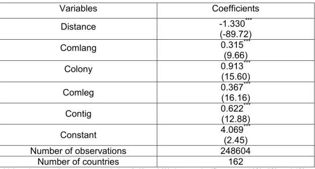
2.5.1. Trade openness, income and FDI equations

All coefficients in the trade gravity equation are highly significant and have the expected sign (Table 2.2).15 Distance has a large and negative impact on bilateral trade. The estimated elasticity of trade openness with respect to distance is slightly higher than one in absolute value. This is not unusual. For example, Feenstra‘s (2004, p.150) distance coefficients/elasticities for trade between US states and Canadian provinces range from -0.79 to -1.42. Finally, sharing the same language, the same colonial history, or having a common legal

15

Trade as well as income and FDI equations are all estimated over the period 1988-2007. A Heckit two-step procedure estimation of the trade equation is used for robustness check and its results are closely similar to their Poisson regression pairs except coefficients on the common colonial dummies which do not have the expected sign. So we rely in what follows on the pseudo maximum likelihood Poisson regression estimation. The PPML procedure is known to yield consistent estimates in the presence of heteroskedasticity.

(39)

system or a common border increase the intensity of trade between two trading partners which is consistent with our priors.

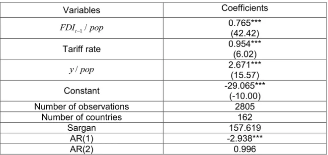
The income and FDI equations are both estimated by GMM. The Sargan test for over-identifying restrictions and the hypothesis of no second-order autocorrelation confirm the validity of the instruments used in the GMM estimation and the absence of serial correlation in the error terms.

As for the trade equation, all estimated coefficients in the income equation are highly significant and have the expected sign (Table 2.4). The estimated coefficient on lagged income (0.90) is strongly significant and reveals a high level of conditional convergence. The estimated coefficient on trade (0.18) means that each 1% increase in trade openness increases income by 0.18 % in the short run and by 1.8 % in the long run.16 The effect of population is negative as predicted by the neoclassical model and, unlike in Frankel and Rose (2005), it is strongly significant. The effects of investment and human capital formation are both positive and the impact of trade and investment on income seems to be of similar magnitude.

The estimated effect of the lagged value of per capita FDI and per capita income are positive and highly significant in the per capita FDI equation (Table 2.5). The effect of the average effective applied tariff is positive and strongly significant which lends support to the tariff-jumping hypothesis. An instantaneous increase of 1% in per capita FDI increases its value by 0.76% after one year and by 3.16 % in the long run.

16 3 0 1 ˆ ln( / ) 0.18 =1.8. ˆ _{1- 0.90} 1 it i y pop T    _ _

  This value is not unusual and is very close to those

(40)

22

2.5.2. The environmental quality equation

We consider three measures of pollution, a global pollutant, CO2, a local pollutant, NO2, and a water pollutant, Biochemical Oxygen Demand (BOD).

2.5.2.1. CO2, NO2 and BOD

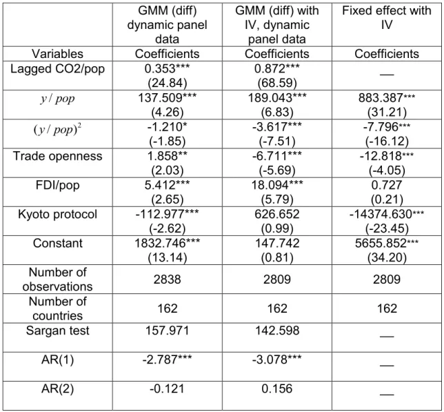
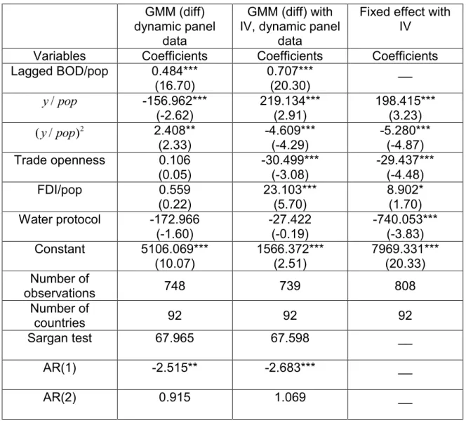
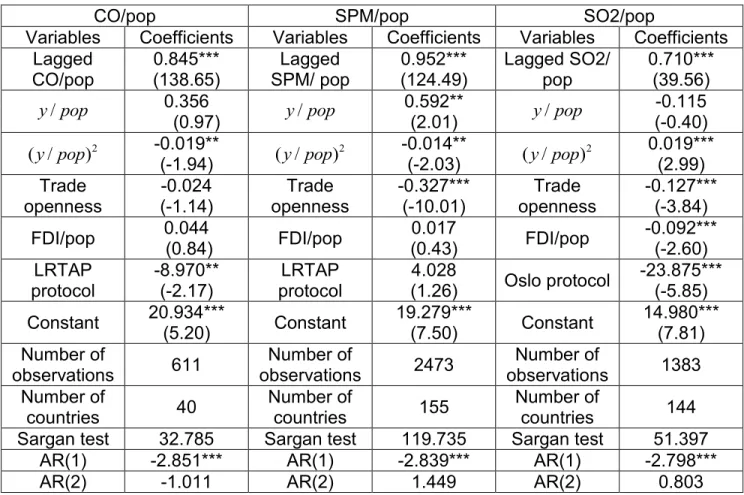
We estimated equation (1) for each pollutant with three different estimators. Tables 2.6.1, 2.6.2 and 2.6.3 respectively present results for CO2, NO2 and BOD. In each table, the first set of result pertains to an estimator that addresses dynamics, but not endogeneity (GMM). The ―middle‖ estimator addresses both dynamics and endogeneity (GMM with IV) while the third set of results are from an estimator (fixed effects) that corrects for endogeneity, but does not allow for dynamics. The Sargan test for over-identifying restrictions and the hypothesis of no second-order autocorrelation confirm the validity of the instruments used in the GMM estimation and the absence of serial correlation in the error terms of all environmental equations.

Starting with our first estimator which allows for dynamics, but does not address endogeneity issues, we notice that the estimated coefficients for per capita income and squared per capita income are respectively positive and negative and hence provide support for the EKC hypothesis for CO2 (table 2.6.1). Increases in per capita income starting from a low level of per capita income tend to increase emissions until a critical per capita income level is reached. Beyond this critical level estimated at $56821, additional increases in per capita income induce decreases in emissions. The estimated coefficients of per capita income are negative in the NO2 equation, indicating that growth is good for the environment. The per capita income coefficients are negative and positive in the BOD equation, signalling the existence of a U-shaped relation between per capita GDP and BOD. This result means that economic growth induces improvements in water quality when the level of per capita income is relatively low and the inverse holds at high levels of per capita income ($32591). The

(41)

estimated coefficient on trade openness is positive in all equations  moderately significant for CO2 and insignificant for both NO2 and BOD pollutants  indicating that trade openness is either bad or of no consequence for the environment. Our central interest is on the coefficient of FDI which is significantly positive in the CO2 and NO2 equations, but not significant in the water pollutant (BOD) equation, when we restrict our attention to specification (I). These findings are generally consistent with the pollution haven hypothesis. The coefficient on the environmental agreement is negative and significantly so for CO2, but not significant for the other two pollutants.

We now assess whether the above results are robust when we use an estimator (GMM with IV) that accounts for dynamics and the endogeneity of real per capita income, per capita FDI, trade openness intensity and the decision to ratify an IEA. For the CO2 equation (2nd column, Table 2.6.1), the coefficients for linear and squared per capita income are still consistent with the existence of an EKC. The income critical levels are estimated at $26182 and $23818 for CO2 and BOD respectively and are so both lower than their non-instrumented counterpart levels. For the BOD equation (Table 2.6.2), the per capita income coefficient is positive and significant when dynamics and endogeneity are accounted for while the squared per capita income remains negative. This supports the existence of EKC curve for BOD. Only the per capita income coefficient is significant in the NO2 equation (Table 2.6.3). We can infer that economic growth causes increases in NO2 emissions, which contrasts with the result from our first estimator.

The pollution haven hypothesis is supported for the global pollutant, as per capita FDI is found to cause increases in CO2 emissions. Carbon dioxide is a global externality and in the absence of international cooperation, countries have less incentive to reduce their emissions through stricter national regulations. Similarly, the impact of FDI on BOD is strongly positive, yielding support for the pollution

(42)

24

haven hypothesis.17_{This result contrasts with the negative impact of FDI on NO2}

emissions, which favors the pollution halo hypothesis. These results suggest that the environmental incidence of FDI varies across pollutants.

Comparing results from the first two estimators in Tables 2.6.1-2.6.3 allows us to gauge the magnitude of the endogeneity biases in estimated coefficients. For CO2, the respective effects of trade openness and Kyoto change from being detrimental and positive to being positive and insignificant. These results are more in line with the theoretical arguments developed by McCausland and Millimet (2012) as to why international trade is easier on the envirionment than intranational trade. For NO2, the effect of trade openness changes from being insignificant to being positive. Frankel and Rose (2005) found a very small impact in the case of NO2 and no impact in the case of CO2 which suggests that the length of our panel matters. In the case of NO2, a sign reversal is observed for FDI. Once endogeneity is corrected, FDI actually reduces emissions. For BOD, FDI and trade openness had no impact according to our first estimator, but the second estimator suggests that trade (FDI) is a friend (enemy) of the environment. The Water protocol does not have an incidence on BOD whether endogeneity is corrected for or not.

We now gauge the importance of dynamics by comparing results of columns 2 and 318 in Tables 2.6.1-2.6.3. Qualitatively, the results for BOD are similar except for the effect of the Water protocol which has no (a significant negative) effect on emission when dynamics are (not) accounted for. The results for NO2 are also similar except for the effect of the Sofia protocol which has a significant negative (no) effect on emission and income coefficients when dynamics are (not) accounted for. The CO2 equation is more problematic for the static estimator because the inference about FDI, trade openness and Kyoto is misleading. The

17_{In many instances, water pollution can easily spread from one country to another, BOD can be}

considered as a global pollutant even though it has also local effects.

18_{Column 3 report the results of specification III, that’s the static version of specification II as cited above,}

(43)

importance of incorporating dynamics is most obvious and this might explain why Frankel and Rose (2005), who worked with a cross-section, have not found evidence supporting the pollution haven hypothesis in any of their instrumented equations.

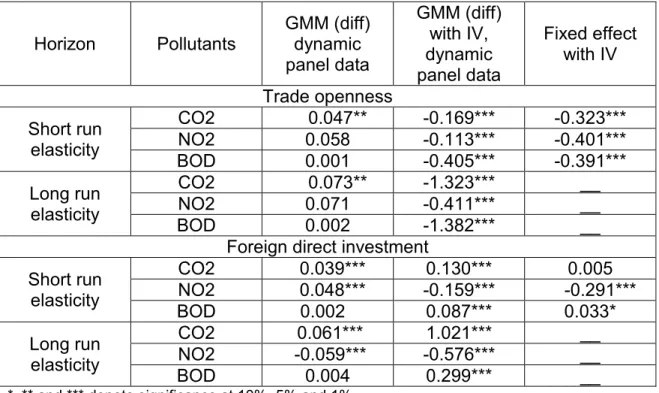
Trade openness being a fraction, its quasi-elasticity, which measures the percentage change in emissions of type j following a 1% increase in trade openness can be computed as: T 100

j

y



 , where _T is the regression coefficient and y is the mean level of emissions of type j. A 1% increase of trade openness _j will in such case increases CO2 emissions by 0.047 % in the short run and by 0.073 % in the long run if endogeneity is not addressed (Table 2.2.7). A 1% increase in trade openness will however decreases CO2 emissions, NO2 emissions and BOD by 0.169 %, 0.113 % and 0.405 % in the short run and by 1.323 %, 0.411 % and 1.382 % in the long run, respectively, when both persistence and endogeneity are considered. Considering only endogeneity will however yield an elasticity of 0.323 %, 0.401 % and 0.391 % of CO2 emissions, NO2 emissions and BOD with respect to trade openness.

Similarly, if we do not address endogeneity, an increase of 1% in FDI increases CO2 and NO2 emissions by 0.039 % and 0.048% in the short run and by 0.061 % and 0.059 % in the long run, respectively; but do not have any effect on BOD (Table 2.7). If we do not consider persistence, an increase of 1% in FDI increases NO2 emissions and BOD by 0.291 % and 0.033 % respectively, but do not have any effects on CO2 emissions. When we address both endogeneity and persistence, an increase of 1% in FDI increases CO2 emissions, NO2 emissions and BOD by 0.130 %, 0.159% and 0.087 % in the short run and by 1.021 %, 0.576 % and 0.299 % in the long run, respectively. We conclude as such that omitting endogeneity under estimated CO2 emissions, NO2 emissions and BOD elasticity with respect to FDI flows. We conclude that omitting endogeneity under estimated both the short and the long run FDI and trade absolute value effects on

(44)

26

CO2 emissions, NO2 emissions and BOD. Omitting persistence make impossible to distinguish between short run and long run effects of FDI and trade openness and underestimated the long run effects of FDI and trade on CO2 emissions, NO2 emissions and BOD. In what follows, we will discuss only from the results obtained with the GMM IV estimator.

From Tables 2.6.1-2.6.3, the long run effect of FDI on CO2 emissions is 7.812 times higher (141.360=18.094/(1-0.872)) than the short run effect (18.094). This implies that a $10 increase in per capita FDI causes per capita CO2 emissions to increase by 180.94 grams in the short run and by 1.413 kg in the long run. On the other hand, the long run effect of FDI on NO2 emissions is 3.610 times (0.512=0.142/(1-0.723)) higher than its short run effect (0.142). This means that a $10 increase in per capita FDI inflows boosts per capita emissions of NO2 by 1.42 gram in the short run and by 5.12 grams in the long run. Finally, the long run effect of per capita FDI on BOD is 3.412 times higher (78.84=23.103/(1-0.707)) than its short run effect (23.103). This means that a $10 increase in per capita FDI inflows increases per capita per day Biochemical Oxygen Demand by 231.03 grams in the short run and 788.4 grams in the long run.

2.5.2.2. Other pollutants

In this subsection, we investigate the impact of trade openness on foreign investment for other global pollutants, HFC-PFC-SF6, Methane and N2O, and three other local pollutants, CO, SPM and SO2. The estimated coefficients reported in Tables 2.8.1 and 2.8.2 for per capita income and its square provide support for the EKC hypothesis for HFC- PFC-SF6, CH4 and SPM. However, we found a linear negative relation for CO and a positive relation for SO2 while N2O emissions do not seem to be affected by growth. The ratification of IEAs has had the desired reducing effect on emissions only for CO and SO2. IEAs do not significantly influence emissions of other pollutants.

(45)

Our results indicate also that trade reduces HFC-PFC-SF6, N2O, SPM and SO2 emissions and decreases the emissions of CH4. FDI tends to increase the emissions of HFC-PFC-SF6, decreases the emissions of SO2 and has no effect on the emissions of other pollutants. These results support the pollution haven hypothesis for global pollutants and the pollution halo hypothesis for local pollutants. Thus it appears that multinational firms introduce technologies in host countries that lead to reduced emissions of local pollutants, but that they cannot prevent global pollutant emissions from growing. The same is true also for water polluting firms. Techniques to increase the quantity of oxygen in water exist, but efficient technologies to reduce the quantity of waste rejected in water itself are lacking. In the absence of international cooperation in dealing with global externalities, it is probably more profitable to promote R&D in local pollutants emitting industries.

2.5.2.3. Trade, growth and FDI effects on pollution by level of development

The results reported in Hoffman et al., (2005) and Hosseini and Kaneko (2012) suggest that the impacts of FDI on pollution can be sensitive to the characteristics of host countries and their level of development. To examine this hypothesis, we divided our sample into developed and developing countries19 and implemented a Wald test to determine whether GMM-IV coefficients differ across subsamples. Results presented in Tables 2.9.1-2.9.5 are for pollutants for which the FDI impact differs across subsamples/level of development. Thus, the pollutants considered are CO2, HFC-PFC-SF6, NO2, BOD and SO2 because the estimated coefficients for ―other pollutants‖ in developed and developing countries were not statistically different. The EKC hypothesis is supported for the CO2 and HFC- PFC-SF6 equations for both developed and developing countries. The critical income levels are evaluated at 27602 $ and 26050 $ in developed and developing countries for CO2, and at 48886 $ and 22457 $ in developed and developing countries for HFC-PFC-SF6. The critical levels are lower in