UNIVERSITÉ DU QUÉBEC À MONTRÉAL
COEXISTENCE ET SYLVICULTURE DE L'ÉRABLE À SUCRE ET DU HÊTRE À GRANDES FEUILLES DANS UN CONTEXTE DE CHANGEMENTS
GLOBAUX
THÈSE PRÉSENTÉE
COMME EXIGENCE PARTIELLE DU DOCTORAT EN BIOLOGIE
PAR
PHILIPPE NOLET
Service des bibliothèques
Avertissement
La diffusion de cette thèse se fait dans le respect des droits de son auteur, qui a signé le formulaire Autorisation de reproduire et de diffuser un travail de recherche de cycles supérieurs (SDU-522 - Rév.0?-2011 ). Cette autorisation stipule que «conformément à l'article 11 du Règlement no 8 des études de cycles supérieurs, [l'auteur] concède à l'Université du Québec à Montréal une licence non exclusive d'utilisation et de publication de la totalité ou d'une partie importante de [son] travail de recherche pour des fins pédagogiques et non commerciales. Plus précisément, [l'auteur] autorise l'Université du Québec à Montréal à reproduire, diffuser, prêter, distribuer ou vendre des copies de [son] travail de recherche à des fins non commerciales sur quelque support que ce soit, y compris l'Internet. Cette licence et cette autorisation n'entraînent pas une renonciation de [la] part [de l'auteur] à [ses] droits moraux ni à [ses] droits de propriété intellectuelle. Sauf entente contraire, [l'auteur] conserve la liberté de diffuser et de commercialiser ou non ce travail dont [il] possède un exemplaire."
REMERCIEMENTS
En tout premier lieu, je désire remercier mon directeur de thèse, Dan Kneeshaw pour ses commentaires et conseils toujours pertinents et constructifs. Côtoyer Dan - un être hors du commun, à la fois grand et simple - au cours des dernières années fut un immense privilège. Je tiens aussi à remercier tous mes collègues à l'ISFORT pour leur soutien et leur encouragement de même que la direction de l'UQO qui m'a permis de compléter ce doctorat dans des conditions plus que favorables. Merci à mes amis et amies qui rn' ont soutenu et surout qui ne rn' ont pas renié malgré le peu de temps que j'avais à leur disposer dans les dernières années. Je veux soulginer l'importance de ma famille, Paule, Danoé et Léry dans cette aventure. Votre présence et votre amour rn' ont permis, malgré la tâche de ce que représente un doctorat, de retrouver chaque jour un hâvre de paix et de rester en contact avec ce qu'il y a de plus important dans la vie.
Enfin, merci à toi, maman, pour la merveilleuse mère que tu as été et pour tout l'amour que tu nous portes encore aujourd'hui à mes frères et moi. Merci à toi papa, fragile et fort dans l'adversité et dont la grandeur du cœur n'a d'égal que celle de ton humilité.
LISTE DES FIGURES ... VI LISTE DES TABLEAUX ... X RÉSUMÉ ... Xll
INTRODUCTION GÉNÉRALE ... 1
CHAPITRE I LIMING HAS A UMITED EFFECT ON SUGAR MAPLE-AMERICAN BEECH DYNAMICS COMPARED TO BEECH SAPLING ELIMINATION AND CANOPY OPENING ... 8 1.1 Abstract ... 9 1.2 Introduction ... , ... 10 1 .3 Methods ... 13 1.3.1 Studyarea ... l4 1.3 .2 Experimental design ... 14 1.3.3 Treatments ... 15 1.3 .4 Field measurements ... 16 1.3.5 Laboratory analyses ... 20 1.3.6 Data analyses ... 20 1.4 Results ... 22
1.4.1 Direct effects of treatments on light environ ment and soit chemistry ... 22
1.4.2 Mature tree radial growth ... 24
1.4.3 Sapling basal area and radial growth ... 26
1.4.4 Seedling abundance and tallest height ... 29
Il
1.5.1 The light-soil interaction hypothesis ... 34
1.5.2 Liming and silvicultural implications ... 36
1.6 Conclusion ... 38
1.7 Acknowledgements ... 39
CHAPITRE II EXTREME EVENTS AND SUBTLE ECOLOGICAL EFFECTS: LESSONS FROM A SUGAR MAPLE-AMERICAN BEECH CASE 2.1 Abstract ... 41
2.2 Significance ... 41
2.3 Introduction ... 42
2.4 Results and discussion ... 44
2.4.1 Growth decline ... 44
2.4.2 Possible causes ... : ... 44
2.4.3 Consequences of the 1986-1989 growth drop ... .4 7 2.4.4 General discussion ... 50
2.5 Methods ... 53
2.5.1 Study area ... 53
2.5.2 Tree sampling ... 53
2.5.3 Data analysis ... 54
CHAPITRE III: COMPARING THE EFFECTS OF EVEN- AND UNEVEN-AGED SILVTCULTURE ON ECOLOGICAL DTVERSJTY AND PROCESSES: A REVIEW 3.1 Abstract ... 59
3.2 lnt::roduction ... 59
3.3 Literature review ... 63
3.3.1 Approach and rationale ... 63
3.3.2 Generalities ... 66
3.3.3 Flora ... 66
3.3.5 Carbon and nutrients ... 70 3.4 Discussion ... 71 3.4.1 Management implications ... 75 3.5 Conclusion ... 79 3.6 Acknowledgements ... 80 CHAPITRE IV CONCLUSION GÉNÉRALE ... 81 APPENDICE A SUPPLEMENT AR Y MA TERJAL TO CHAPTER I ... 88
APPENDICE B SUPPLEMENT AR Y MA TERJAL TO CHAPTER II ... 94
APPENDICE C SUPPLEMENT AR Y MA TERI ALTO CHAPTER Ill ... 102 LISTE DES RÉFÉRENCES ... 121
Figure Page Figure 1.1 Sampling and treatment design used in each treatment unit. ... 15 Figure 1.2 Light availability as a function of canopy opening and beech sapling
elimination treatments. The limits ofthe box are the 25 and 75 percentiles, the separating line between the two shades of grey is the median, the lower and upper limits ofthe whiskers are the lOth and 90th percentiles, and points are beyond 1.5 x the interquantile range (25t11-751h percentiles) ... 23 Figure 1.3 Effect of liming on Ca and Mg concentrations and on pH. Details of the
box plots are included in Figure 1.2 ... 24 Figure 1.4 Mature tree radial growth change between pre and post treatment periods
for sugar maple (SM) and American beech (AB) according to the canopy opening and liming treatments. Percentages related to L, B, CO represent their respective cunmlative probabilities to be included in the best model (see Methodology and Table 1.3 for details). The percentage associated with the intercept is provided for comparison. Details of the box plots are included in Figure 1.2 ... 25 Figure 1.5 Sapling radial growth change between pre- and post-treatment periods
for sugar maple (SM) and American beech (AB) according to the canopy opening and liming treatments. Percentages related to L, B, CO represent the cumulative probabilities that liming, sapling beech elimination, and canopy opening treatments would be respectively included in the best model that was tested for a species (see Methods and Table 1.3 for details). The percentage associated with the in terce pt is provided for comparison. Details of the box plots are included in Figure 1.2 ... 28 Figure 1.6 Difference in seedling density before and after treatment according to the
various treatments for sugar maple (SM) and American beech (AB). Au: Autumn; Su: late-summer. Percentages related to L, B, CO represent the cumulative probabilities that liming, sapling beech elimination, and canopy
Vll
opening treatments would be respectively included in the best mode! that was tested for a species (see Methods and Table 1.3 for details). The percentage associated with the intercept is provided for comparison. Details of the box plots are included in Figure 1.2 ... 30 Figure 1.7 Mean height ofthe tallest seedling in each subplot for the various
treatments for sugar maple (SM) and American beech (AB). The fitted values refer to the predicted values at the plot leve!, after taking into account the random effect. Percentages related to L, B, CO represent the cumulative probabilities that liming, sapling beech elimination, and canopy opening treatments would be respectively included in the best mode! that was tested for a species (see Methods and Table 1.3 for details). The percentage associated with the intercept is provided for comparison. Details of the box plots are included in Figure 1.2 ... 31 Figure 1.8 Percentage of each species having the dominant individual seedling in
subplots according to the various treatments. SM: sugar maple; AB:
American beech OS: Other species. Percentages related to L, B, CO represent the cumulative probabilities that liming, sapling beech elimination, and canopy opening treatments would be respectively included in the best mode! that was tested for a species (see Methods and Table 1.4 for details). n = 85, 70 and 75 respectively for controls, selection cuts and clear-cuts ... 33 Figure 2.1 Radial growth comparison between sugar maple and American beech
over a 60-year period. A): absolute values B) relative values, a negative value signifies a lower growth for sugar maple; the grey boxes indicate confidence intervals at 95%. C) Mean sugar maple and American beech radial growth by DBH class. Black and blue arrows (panel A) respectively indicate drought and thaw-freeze events as indicated by daily meteorological data (see methods and supplementary information). Red lines (panel A) show
documented forest tent caterpillar outbreaks (see methods) ... 46 Figure 2.2 Sugar maple and American beech detrended growth indices as a function
of mean June temperature and June-July precipitation. R2 are provided for simple regressions while adjusted R2 are provided for multiple regressions. None of the multiple regression analyses for American beech are shown as they did not explain any further variation in growth. Trend lin es show significant (p < 0.05) simple linear relationships. Climate variables are presented in Figure B.4 ... 49 Figure 2.3 Relative radial sugar maple growth drop in 2006-2007 as a function of
show significant (p < 0.05) simple linear relationships. See methods for details on relative growth radial calculations ... 50 Figure 3.1 Schematic representation ofthe difference in the landscape structure
between A) even-aged and B) uneven-aged silviculture. In even-aged silviculture, trees in each stand are surrounded by trees with similar ages and heights while in uneven-aged silviculture, trees are surrounded by trees of varying ages and heights. In both cases, smaller trees are expected to replace larger trees once the latter are harvested ... 62 Figure 3.2 Approximate location and species composition of the reviewed studies in
relation to forest biomes. The term "various" means that studies were
conducted in more than one forest composition ... 66 Figure 3.3 Simulated landscape scale ecologicallong-term impact ofEAS and UAS
(C) based on hypothetical short-term impacts ofUAS as 80% ofthat ofEAS hypothetical short-term impacts (A) and recovery rates (B). A) shows that short-term impacts (hypothetical variable) differ strongly at the landscape level between EAS and UAS because more surface is affected by forestry operations to harvest the san1e wood volume each year when UAS is used. B) Recovery rates: for UAS the theoretical recovery rate shown is such that at the end of a 20-year cutting cycle, the hypothetical variable recovered to its pre-harvest state; for EAS, two recovery rates are provided: 'li and ~ the recovery rates ofUAS ... 74 Figure 4.1 Liens entre les chapitres de la thèse à travers certains résultats
importants ... 86 Figure 4.2 L'intervention ou l'abstention sylvicole face aux changements globaux
régentée selon quatre principes ... 87 Figure A.1 Study site and treatment units localisation ... 89 Figure A.2 Modified leaf blower. We added a two-entry conduct to the original
tube of the blower. The lime was incorporated in the 45° angle entry and then blown in the forest stand ... 91 Figure A.3 Boxplots of sugar maple (SM) and American beech (AB) sapling basal
area development according to the various treatments. Au: Auturnn; Sp: Spring; Su: late-surnmer. Percentages related to L, B, CO represent the cumulative probabilities that the liming, sapling beech elimination, and canopy opening treatments be respectively included in the best model (see Methodology and Table 1.3 for details). The percentage associated to the
lX
intercept is provided for comparison. Details of the box plots are included in Figure 1.2 ... 92 Figure A.4 Evolution of seedling density for sugar maple (SM) and American beech
(AB). Only data without liming and AB sapling elimination are presented. Au: Auturnn; Sp: Spring; Su: late-surnmer. ... 93 Figure B.1 Mean diameter and mean radial growth of 34 dominant sugar maple
(DBH >44 cm in 2012) trees on a 60-year period. Trees were sampled in the same stands than th ose of Figure 2.1. Radial growth of these sugar maples when they had 40 cm in DBH (~ 1972) was about 2.2 mm*year-1, which is much higher than the growth oftrees ofthe same size nowadays (Figure 2.1C) ... 95 Figure B.2 Y ear of establishment for 40 sugar maple sampled in 2001 ... 96 Figure B.3 Detrended growth indices for sugar maple (orange) and American beech
(green) for the 1948-2007 period ... 97 Figure B .4 Climate variables from 1948 to 2007. Only the climate variables used in
Figure 2.2 and Table B.1 are shawn ... 99 Figure B.5 Daily precipitation during the months of May to July for drought years
between 1948 and 2007 according to the Mont-Laurier weather station. The grey line indicates mean daily precipitation over the period. Arrows show the periods of drought. See methodology for definition of a drought year ... 100 Figure B.6 Thaw-freeze events described by thaw length and subsequent
temperature drop, each point representing a precise date between 1950 and 2007 for the months of January and February ... 101
Tableau Page Table 1.1 Number oftreatment units (n) and mean pre-harvest basal area in sugar
maple (SM) and American beech (AB) by treatment combinations ... 18 Table 1.2 Chronology of treatments and data collected during the present study ... 19 Table 1.3 Mode! comparison for mature tree growth, sapling basal area, sapling
radial growth, seedling density and seedling height and for each species .... 27 Table 1.4 Model comparison for the multinomiallogistic regressions used to predict the species with the dominant seedling at the subplot lev el. ... 32 Table 3.1 Literature comparing even- and uneven-aged silviculture for tree species
diversity ... 65 Tableau 3.2 Questions for guiding the use of even- and uneven-aged silviculture in
a given region ... 79 Table A.1 Mode! comparison for light, Ca, Mg and pH ... 90 Tableau B.1 Correlation between climate variables and growth indices for sugar
maple and American beech. Only months where correlations> 0.33 for the 1950-1985 period are shown. Correlations were performed using the climate variables from both the growth year ( current) and the year prededing the growth (-1) ... 98 Table C.l Literature comparing even-and uneven-aged silviculture for herbs and
shrubs ... 103 Table C.2 Literature comparing even- and uneven-aged silviculture for structural
elements ... 1 06 Table C.3 Literature comparing even-and uneven-aged silviculture for mycorhizae,
Table C.4 Literature comparing even- and uneven-aged silviculture for marnmals 109
Xl
Table COS Literature comparing even- and uneven-aged silviculture for birds 0 0 0 0 0 111 Table Co6 Literature comparing even-and uneven-aged silviculture for herpsooooo 113 Table Co7 Literature comparing even- and uneven-aged silviculture for invertebrates
115
Table Co8 Literature comparing even- and uneven-aged silviculture for respiration and carbon sequestration 0 0 0 0 0 0 0 0 0 0 0 0 0 0 0 0 0 0 0 0 0 0 0 0 0 0 0 0 0 0 0 0 0 0 0 0 0 0 0 0 0 0 0 0 0 0 0 0 0 0 0 0 0 0 0 0 0 0 0 0 0 0 0 0 0 0 0 0 0 0 0 0 0 0 0 0 0 117 Table Co9 Literature comparing even- and uneven-aged silviculture for soil water
La présente étude visait à mieux comprendre la dynamique de la coexistence entre l'érable à sucre (Acer saccharum Marsh.) et le hêtre à grandes feuilles (Fagus grandifolia Ehrh.) dans un contexte de changements globaux et à évaluer des pratiques sylvicoles pouvant être adaptées à cet écosystème dans ce contexte en perpétuel changement. Dans le premier chapitre, nous nous sommes intéressés à l'effet de la fertilisation sur la croissance et la régénération de ces deux espèces dans un contexte où plusiems autems émettent l'hypothèse d'une baisse de fertilité des sols- en raison des précipitations acides-qui défavoriserait l'érable aux par rapport au hêtre à grandes feuilles. Les données provenant d'une dispositif de fertilisation (chaulage) ne montrent que des effets négligeables de ce traitement sur la dynamique entre les deux essences, alors que des traitements de récolte et d'élimination des gaules de hêtre ont des effets beaucoup plus marqués. Nos résultats ne semblent pas démontrer que la richesse des sols est un facteur limitant la croissance et la régénération de l'érable à sucre dans la région à l'étude.
Dans le deuxième chapitre, nous nous sommes penchés sur l'évolution comparée de la croissance de l'érable à sucre et du hêtre sur une période d'environ 60 ans par dendrochronologie. Nos résultats démontrent clairement une chute abrupte de la croissance de 1' érable par rapport au hêtre à partir de 1986. Sans pouvoir 1' affirmer avec certitude, nous émettons l'hypothèse que cette baisse de croissance serait due à un événement de redoux suivi d'un gel sévère en janvier 1986, puis suivi par une sécheresse en 1988. Non seulement l'érable à sucre n'a pas recouvré sa croissance 20 ans plus tard, mais il semble avoir été affecté de nouveau par un autre événement extrême. Comme les événements extrêmes sont appelés à être de plus en plus fréquents, mais qu'ils peuvent avoir des effets en apparence subtils, nous prônons le développement d'approches de modélisation novatrices qui permettront de prendre en compte les effets de tels événements.
Dans le troisième chapitre, nous nous sommes intéressés à l'aménagement équienne comme outil potentiel pour l'adaptation aux changements globaux puisque ce mode d'aménagement est presqu'inutilisé dans les érablières du Québec. L'aménagement
Xlll
équiem1e présente 1 'avantage de favoriser une grande diversité - tant à 1' échelle du peuplement que du paysage - qui est souvent vue comme un élément important de la résilience des forêts face aux changements globaux. Malgré l'absence de littérature sur le sujet, il existe une forte croyance à l'effet que l'aménagement inéquienne est préférable à l'aménagement équienne pour favoriser la résilience des forêts. Nous avons ainsi procédé à une revue de littérature recensant les articles scientifiques à travers le monde qui comparent les deux modes d'aménagement au niveau écologique. Il ressort de cette revue qu'aucune des deux approches ne semble supérieure à l'autre du point de vue écologique, chacune ayant ses avantages et inconvénients. Comme les réponses obervées sur les effets de 1 'aménagement équierme et inéquienne sont très spécifiques aux espèces, cette revue supporte qu'une diversité d'approches sylvicoles sont nécessaires pour maintenir une diversité d'habitats. Par le fait même, notre étude ouvre la voie pour les aménagistes à l'utilisation d'un outil sylvicole supplémentaire-l'aménagement équienne, qui était quasiment proscrit dans certains types de forêts (ex. : les forêts de feuillus nobles)- pour faire face aux changements globaux.
Pris dans leur ensemble, les résultats des chapitres de la thèse supportent 1 'utilisation mesurée de 1 'aménagement équienne dans les érablières pour, entre autres, favoriser l'érable à sucre aux dépens du hêtre et la résilience de cet écosystème dans son ensemble. Enfin, nous jetons les bases d'une approche permettant de doser le niveau d'interventionnisme de l'humain dans sa volonté de faciliter l'adaptation des écosystèmes forestiers aux changements globaux.
La coexistence des espèces intrigue les écologistes depuis des décennies (ex. (Whittaker, 1965); elle a été étudié dans plusieurs milieux (ex. Christie and Armesto, 2003; Lusk and Smith, 1998; Wright, 2002; Yamamoto et al., 1995), et pour plusieurs taxa (ex. Martin, 1988; Novotny et al., 2002; Pfennig et al., 2006). Aussi, la coexistence des espèces est un çhamp de recherche en lui-même. Par exemple, Zobel (1992) identifie sept concepts (complémentaires ou exclusifs) permettant d'expliquer la coexistence d'espèces. Dans les dernières années, la théorie du modèle neutre (Hubbell, 1997) est certes celle qui a attiré le plus d'attention (Grave! et al., 2006). Cette théorie est à 1 'opposé de celle des niches et considère les espèces comme équivalentes au niveau fonctionnel et elle prend en compte les dynamiques aux échelles de la population locale et. de la métacommunauté. Toutefois pour qu'une coexistence s'installe, une stabilité est requise dans les forces qui structurent les commw1autés (Clark et al 2007). Or, cette stabilité, spécialement avec les changements globaux, est fortement remise en question.
Depuis plusieurs décennies, les scientifiques tentent d'expliquer la coexistence de l'érable à sucre et du hêtre à grandes feuilles (CEEH) dans les forêts tempérées du nord-est américain. On parle de coexistence plus que de succession (e.g. Forcier, 1975) parce que les deux essences sont très tolérantes à l'ombre et qu'aucune ne semble dominer au point de marginaliser l'autre tant à l'échelle du peuplement que du paysage, et ce sur une longue période (plusieurs siècles). C'est la définition que nous retiendrons pour cette thèse. Poulson et Platt (1996) ont proposé un modèle de coexistence allogénique, dépendant de la grandeur et de la fréquence des trouées. Ce
2
modèle se situe dans le même courant que celui des études de Runkle (1981) et Canham (1988, 1989) qui ont aussi étudié le succès de la régénération de ces deux essences en fonction de diverses caractéristiques des trouées. Bien que les résultats de ces études ne soient pas toujours concordants, ils tendent généralement à démontrer que le hêtre a une meilleure capacité à survivre sous couvert et que l'érable à sucre a une meilleure capacité à augmenter sa croissance en hauteur en présence d'une trouée. Par contre, Beaudet et al. (2007) n'observent pas de changements marqués de la performance de la régénération des deux essences selon un gradient de lumière après une importante ouverture créée par un verglas. Ce résultat est en contradiction avec celui de Canharri (1989) qui a observé une meilleure réponse de la part de l'érable à des petites trouées que de la part du hêtre. Nolet et al. (2008) observent un plus grand succès pour l'érable à sucre après coupe totale qu'après coupe partielle et émettent l'hypothèse qu'il existe un seuil de lumière à partir duquel l'érable à sucre est plus performant que le hêtre à grandes feuilles. Ce seuil serait toutefois beaucoup plus élevé que celui proposé par Poulson et Platt (1996). (Grave! et al., 2011) observent un changement sur 40 ans dans le succès relatif de l'établissement des deux essences, passant d'un avantage pour l'érable à un avantage pour le hêtre à grandes feuilles sans toutefois pouvoir en expliquer les causes. Arii et Lechowicz (2002) ont quant à eux démontré que les conditions de sol avaient aussi un effet important sur le succès de régénération des deux essences, le hêtre évitant les sites les plus secs et l'érable évitant les sites plus pauvres (pH acide et teneur en calcium plus faibles) sous la canopée de hêtre. Ce dernier résultat, l'effet de la canopée du hêtre sur les caractéristiques des sols, va dans le sens d'une coexistence autogénique et est donc en contradiction avec le modèle de Poulson et Platt. D'autres auteurs ont aussi vu des relations entre les caractéristiques de sol et le succès relatif des deux essences en régénération (Duchesne et al., 2005; Nolet et al., 2008) alors que d'autres n'en ont pas observées (Grave! et al., 2011).
Parallèlement aux études sur la CEEH, de très nombreuses études se sont penchées sur le dépérissement de la cime ou le déclin de la croissance de l'érable à sucre observé à différentes périodes dans le nord-est américain et au Canada depuis quelques décennies (Millers et al., 1989). Il n'est pas toujours facile de dissocier les phénomènes de dépérissement et déclin puisqu'ils sont intimement liés (Houston, 1999). La quantification de ces phénomènes prend différentes formes. Par exemple, sur le plateau des Appalaches, les érables morts peuvent représenter de 25 à 30% de la surface tenière en érable sur les certains sites les plus susceptibles (Hallett et al., 2006). Bauce and Allen (1991) observent une diminution de croissance en surface terrière de l'érable dans l'état de New York de l'ordre d'environ 40% entre 1962 et 1987. Duchesne et al. (2002) ont aussi observé de telles chutes de croissance dans certains sites du Réseau d'étude et de surveillance des écosystèmes forestiers (RESEF) du Québec. Kolb et McCormick (1993) montrent une baisse de croissance en surface terrière d'environ 75% sur 20 ans dans des érablières de la Pennsylvanie. Ce ne sont pas toutes les régions qui sont touchées par le déclin/dépérissement; par exemple, Lane et Reed (1993) n'observent aucun signe de déclin à long terme pour l'érable dans le nord des États-Unis. Dans l'ouest du Québec, des données récentes semblent indiquer que la croissance en diamètre de l'érable à sucre est toujours en déclin (Labrecque et al., 2006).
Ce déclin/dépérissement a été associé à de nombreux facteurs, tels la défoliation par l~s insectes (Cooke and Lorenzetti, 2006), les maladies (Houston, 1999), les facteurs climatiques (Auclair et al., 1996; Payette et al., 1996), les dépôts acides (Adams, 1999), la densité des peuplements (Bauce and Allen, 1991), l'âge des peuplements (Auclair et al., 1996) et la colonisation par l'érable de sites qui lui sont peu propices (Horsley et al., 2000). Il demeure que les chercheurs semblent s'accorder sur le fait qu'il n'y a pas qu'une seule cause liée au déclin de l'érable à sucre. Toutefois, c'est sur 1' importance relative de ces facteurs ou leur caractère (facteur prédisposant,
initiateur, aggravant (Manion, 1981) que les opinions divergent. Les facteurs liés aux peuplements (densité, âge et qualité de site) sont considérés comme des facteurs prédisposant en ce sens qu'ils ne sont pas à l'origine du dépérissement, mais le favorisent. Les défoliations par les insectes (Gavin et al., 2008) ont des effets marqués sur la croissance de l'érable, mais je n'ai trouvé aucune étude qui présentait cette cause comme étant la principale cause du déclin/dépérissement de l'érable à sucre. Les défoliations par les insectes semblent souvent agir en concomitance avec
des événements climatiques extrêmes. Pour plusieurs auteurs, les événements
climatiques extrêmes seraient la cause principale des déclins observés (Auclair et al., 1997; Bauce and Allen, 1991; Gavin et al., 2008); les sécheresses et les événements de gel-dégel sont les phénomènes les plus souvent cités. Enfin pour plusieurs autres chercheurs, les dépôts acides, en diminuant la quantité d'éléments nutritifs disponibles dans le sol pour la végétation, seraient la principale cause de dépérissement des érablières (Adams, 1999; Moore et al., 2012; Sharpe et al., 2002). Le débat sur 1' importance des dépôts acides sur la santé et la dynamique des érablières a d'ailleurs donné lieu à des échanges virulents dans la littérature scientifique (Messier et al., 2011; Sharpe et al., 2002).
En général, les corpus de littérature sur la CEEH et le dépérissement des érablières sont très indépendants, peu d'auteurs faisant le lien entre les deux sujets (voir toutefois Duchesne et al., 2005 et ~olet et al., 2008). Cela s'explique probablement par le fait que les études traitant de la CEEH ont en commun qu'elles ne regardent que le succès relatif de la régénération (semis et gaules) d'une essence par rapport à l'autre. Bien qu'il soit extrêmement pertinent de s'intéresser à la régénération pour connaître comment évolue la dominance entre les deux essences, il est surprenant que peu d'études (voir Runkle, 2013) se soient penchées sur la performance relative des deux essences à des stades J?lus avancés (DHP de 10 cm et plus). Cette performance à des stades plus avancés, certes influencée par le dépérissement, est
susceptible d'influencer la composition en essences dans la canopée, qui, à son tour, peut avoir une influence sur le succès de régénération des deux essences.
Afin de mieux comprendre l'évolution de la CEEH dans un contexte de changements globaux, la présente étude vise à préciser l'effet des variables climatiques et du statut nutritionnel, appelés à évoluer avec les changements climatiques et les dépôts acides (deux des éléments les plus importants des changements globaux), sur la CEEH, et ce, à différents stades de développement des individus, pas seulement au stade de la régénération. La prise en compte de différentes classes de taille des individus dans l'étude de la CEEH apparaît importante pour deux raisons distinctes. Premièrement, les individus dominants de la canopée ne sont pas soumis aux mêmes conditions de croissance que les individus sous la canopée que ce soit en termes de radiation, de température, de pression atmosphérique ou de vitesse de vent (ex. Baldocchi et al., 2002). N'étant pas soumis aux mêmes conditions, les individus de différentes tailles ne réagiront pas nécessairement de la même façon à des changements de conditions (ex.: disponibilité en eau - Mérian and Lebourgeois, 2011 - ou en éléments nutritifs). Deuxièmement, le stade de développement ontogénique peut avoir un effet marqué sur l'allocation des ressources (Delagrange et al., 2004). Il est donc logique de croire que des individus de tailles différentes ne sont pas nécessairement influencés de la même façon par des changements de conditions de croissance. Par exemple, des jeunes tiges en plein développement pourraient avoir des besoins en éléments nutritifs du sol plus grands que des arbres dominants qui, en grande partie, recyclent les éléments nutritifs (Vadeboncoeur, 2010). Autre exemple, des plus petits individus ayant des systèmes racinaires moins bien développés pourraient avoir plus de difficultés à tolérer un déficit en eau.
Par ailleurs, les changements globaux ne sont pas les seuls facteurs à influencer la CEEH puisque d'autres facteurs, tels les épidémies d'insectes (Cooke and
Lorenzetti, 2006), le broutage par les chevreuils (Sage et al., 2003), et l'aménagement forestier (Nolet et al., 2008), peuvent aussi influencer cette coexistence, et ce, de façon indépendante ou non des changements globaux. L'aménagement forestier, et plus spécifiquement la sylviculture, peut toutefois constituer une opportunité pour rendre les forêts plus résilientes face aux changements globaux. Toutefois dans la très grande majorité des juridictions qui couvrent l'aire de distribution de 1 'érable à sucre et du hêtre à grandes feuilles, la sylviculture est peu diversifiée puisque l'aménagement inéquienne (coupe de jardinage) y est fortement recommandé, sinon obligatoire, ne laissant que très peu de place à l'aménagement équienne. Pourtant, l'an1énagement équienne, spécialement s'il est bien agencé avec d'autres formes d'aménagement, semble présenter certains avantages en termes de résilience des peuplements forestiers, car il favorise souvent une diversité en essences forestières et permet de ré-initialiser un peuplement forestier à partir de jeunes tiges vigoureuses. Dan un contexte de changements globaux, une diversification de la sylviculture favoriserait probablement la résilience des écosystèmes présentement dominés par ces deux essences. Or, l'aménagement équienne se bute à des préjugés quant à ses impacts écologiques-peut-être parce qu'utilisé de façon trop dominante dans cet1aines régions. Si ces préjugés sont fondés ou demeurent des préjugés, il sera difficile d'entrevoir l'aménagement équienne comme une option valable pour favoriser la résilience des forêts
Ainsi, dans le Chapitre 1, j'étudierai la comment la CEEH est influencée par des changements dans le statut nutritionnel du sol en relation avec la taille des individus. Dans le Chapitre 2 de ma thèse, je me pencherai sur les effets du climat sur la CEEH en fonction de la taille des individus étudiés (contrairement à Gravel et al. (20 11) par exemple qui s'étaient concentrés sur les gaules). Finalement, dans le Chapitre 3, j'évaluerai, à partir d'une revue de littérature, comment l'aménagement équienne et inéquienne se comparent quant à letirs impacts écologiques dans les forêts du monde
entier.
Mes hypothèses générales sont dont les suivantes:
• Comme de nombreuses études tendent à démontrer un effet positif important de la fertilité des sols sur 1' érable à sucre, la fertilisation devrait favoriser la croissance et la régénération de l'érable à sucre aux dépens du hêtre à grandes feuilles.
• Comme de nombreuses études ont relaté une baisse de croissance de 1' érable
à sucre, et ce un peu partout sur son aire de distribution, un moment charnière relié au début de cette baisse devrait être observé;
• Comme 1 'aménagement équienne est perçu de façon négative au Québec (en forêt feuillue noble plus particulièrement) et dans plusieurs autres juridictions, une revue de littérature exhaustive comparant les effets écologiques de l'aménagement équienne et inéquienne devrait démontrer des effets écologiques beaucoup plus négatifs pour l'aménagement équienne.
CHAPITRE I
LIMING HAS A LIMITED EFFECT ON SUGAR MAPLE-AMERICAN BEECH DYNAMICS COMPARED TO BEECH SAPLING ELIMINATION AND CANOPY
OPENING.1
1 Ce chapitre a été accepté, tel que présenté, dans la Revue canadienne de la Recherche forestière. Les co-auteurs sont : Sylvain Delagrange, Kim Bannon, Christian Messier et Daniel Kneeshaw.
1.1 Abstract
Sugar maple (SM, Acer saccharum Marsh.)-dominated forests of North America are increasingly affected by many human-induced modifications in environmental conditions. As a remedy, adapted silvicultural treatments are needed. Even though it is generally accepted that SM health is related to soil fertility and that there is an extensive literature on SM-American beech (AB, Pagus grandifolia Ehrh.) regeneration stand dynamics related to light availability, the interaction between these two factors bas rarely been studied. Our main objective was thus to verify the possible role of a light-soil interaction on SM-AB stand dynamics. We used a factorial design with three factors (harvest intensity, liming and beech sapling elimination) to test this interaction. Our results showed that the radial growth of SM and AB tree and sap ling growth was positively affected by canopy opening but not by liming. Liming did not favour AB seedlings while it favoured SM in specifie canopy opening situations confirming, albeit partially, the light-soil interaction hypothesis. Overall, liming bad very limited effects on SM-AB stand dynamics compared to canopy opening and AB sapling elimination treatments. We do not advocate the extensive use of liming as other silvicultural strategies tested provided more promising results to favour SM over AB.
10
1.2 Introduction
For decades, forest ecologists have attempted to understand the mechanisms that drive changes in forest composition in order to predict future conditions. This understanding is crucial in an era of global change, given that silvicultural treatments
can either help forests to adapt to novel ecological conditions (e.g. West et al., 2009)
or decrease forest resilience when improper actions are taken. The forests of northeastern North America that are dominated by sugar maple (SM, Acer
saccharum Marsh.) represent an example of an ecosystem that requires both deeper
understanding and adapted silviculture, as evidence shows that this ecosystem bas already been affected by changes in environmental conditions (e.g. Auclair et al.,
1996; Driscoll et al., 2003). Despite many studies that have been carried out on the
dynamics of sugar maple-dominated ecosystems in the last few decades, limited links have been made between two major research perspectives: the first one, driven main! y by abiotic factors ( e.g. soi! fertility ), focuses on sugar maple decline and the
second one driven, main! y by biotic factors, focuses on sugar maple-American beech
(AB, Fagus grandifolia Ehrh.) coexistence.
SM decline has been reported in many studies over recent decades. This decline,
which is closely linked to SM dieback (Houston, 1999), has affected SM stands in
many parts of its distribution. For example, Hallett et al. (2006) reported that dead
SM represent about 25% to 30% of SM basal area on the Allegheny Plateau of the
northeastern USA. Moreover, mahy studies have reported decreases in basal areal
increment in recent decades: a decrease of approximately 30% in the state of New York (Bauce and Allen, 1991) and in the province of Québec (Duchesne et al., 2002),
While it is generally accepted that SM decline is due to many concomitant factors -insect defoliation (Cooke and Lorenzetti, 2006), diseases (Houston 1999), climatic
events (Auclair et al., 1996; Payette et al., 1996), soil fertility depletion is the factor
that has received the most attention. Many studies (Duchesne et al., 2002; Hallett et al., 2006; Kolb and McCormick, 1993) have shown a relationship between sugar
maple decline and current soil nutrient status (mainly with Mg and Ca). However, these studies could not determine a causal relationship because they did not directly link SM decline to any change in soil nutrient status. To overcome this problem, many studies have tested whether fertilization would increase SM performance. In
a meta-analysis, Vadeboncoeur (2010) showed that fertilization with Ca (alone or in
combinations with other elements) generally has a positive effect on SM performance. However, results were highly variable as sorne authors observed marked positive effects (Long et al., 2011; Moore and Ouimet, 2006; Wilmot et al., 1996), others observed no effects (Fyles et al., 1994; Gasser et al., 2010), and still others noted negative effects (Côté et al., 1995). In another recent meta-analysis, Reid and Watmough (2014) also observed strong variation in the effects of liming
and ash fertilization on hardwood growth.
On the biotic side, many studies published since the early 1980's focused on
SM-AB coexistence. While sorne divergent results have been reported, a consensus seems to emerge- especially among studies focussing on the regeneration dynamics between the two species, that a slight increase in the frequency and size of gaps favours SM over AB. For example, Runkle (1981) showed that the SM-AB dynamics differed among sites given that species self-replacement occurred on sorne sites while reciprocal replacement of SM by AB regeneration occurred on others. Canham (1988) observed a stronger growth response of SM than AB to small canopy gaps, which he attributed to a greater increase in leaf area and better leaf display for
12
sugar maple in gaps compared to those beneath closed canopies. He subsequently
showed that beech saplings are better able to withstand canopy competition
(Canham, 1990). Brisson et al. (1994) predicted that in an old-growth SM dominated
stand, AB abundance would strongly increase if the high proportion of AB that was
observed in the sapling layer persists. The authors further suggested that light was a possible limiting factor for SM seedling survival. Poulson and Platt (1996) observed that an increase in the number of gap openings and available vertical light in the recent decades shifted SM-AB dynamics, leading to an advantage of SM over AB.
In subsequent decades, a number of studies arrived at different conclusions. Beaudet
et al. (2007), who worked on the.same site as Brisson et al. (1994), noticed no
significant changes in the relative performance of SM and AB seedlings after large openings were created by a severe ice storm. Nolet et al. (2008) showed openings that were much larger than those described by Poulson and Platt (1996) or Canham (1988) were required to favour SM over AB in the sapling stage. Nelson and Wagner (2014) observed that shelterwood harvests are not sufficient to favour SM over AB
at the seedling stage unless a silvicultural treatment is applied to eliminate the AB
sapling layer. To understand how SM can be promoted at the expense of AB is
actually an important issue because SM has a much greater economie value.
Studying the combined effect of stand disturbance history and soi! nutrient status on current SM and AB regeneration, Nolet et al. (2008) put forward a hypothesis that would help to reconcile differences in findings from studies that were related to SM-AB dynamics with those that were related to the effect of soil fertility on SM decline. Their hypothesis considers a light-soil interaction and is two-fold. First, as light increases, SM performance relative to that of AB improves and, beyond a certain threshold, SM even exceeds AB growth. While other authors had found similar
results, Nolet et al. (2008) add that this threshold is much higher than previously found and that large openings are required for SM to outperform AB. The second part of the light-soil interaction hypothesis predicts that the light threshold is higher on less fertile sites, meaning that on poorer soils, SM will require more light to outperform AB. This second part is in agreement with many findings showing SM to be more sensitive to changes in soil fertility than AB (Kobe et al., 2002; Long et al., 1997). This hypothesis is supported physiologivally as nutrients (e.g calcium) are involved in several leaf mechanisms including stomata opening and synthesis of membanes and cell walls (McLaughlin and Wimmer, 1999). ·Furthermore, Nolet et al. (2008) were not explicit about how their hypothesis might apply to various stages of stem development. However, the consideration of stem size in the study of SM-AB dynamics appears to be important for two distinct reasons. First, dominant individuals in the canopy are not subject to the same growth conditions as individuals under the canopy (poles, saplings and seedlings) in terms of radiation, temperature, air pressure or wind speed (e.g., Baldocchi et al. 2002). Second, the stage of development of the individual (or size) can have a marked effect on resource allocation (Delagrange et al., 2004). It is therefore logical to assume that individuals of different sizes are not necessarily influenced in the same way by changes in growth conditions (Mérian and Lebourgeois, 2011). A better understanding of how the response of the various stages of stem development to canopy opening and fertilization differ is crucial to develop sound silvicultural treatments.
Using an experimental design that was established in 2006, our objectives were i) to test the light-soil interaction hypothesis advanced by Nolet et al. (2008) and ii) to propose adapted silvicultural treatments to favour SM at the expense of AB.
14
1.3.1 Study area
The study area is located northeast of Duhamel (Quebec, Canada) close to Gagnon Lake (46°07'40" N, 75°09'24" W.), which is in the eastern portion of the Simon Lake
landscape unit in the western sugar maple-yellow birch (Betula alleghaniensis Britton)
bioclimatic region (Saucier et al., 2009).The landscape contains numerous hills with
elevations rarely exceeding 350 rn asl (Robitaille and Saucier, 1998). Mean annual
temperature is 3.7 °C, the mean annual precipitation is about 1000 mm (including 250
mm as snow), and the number of degree-da ys above 0 °C is 2716 (Environment Canada, 2014). Surface geology of the study area is characterized by thin to moderately thin
glacial till, which is composed of metamorphic rocks, such as gneiss. The parent
material is topped by sandy Dystric Brunisols (Soil Landscapes of Canada Working
Group (SLCWG), 2010). The forest canopy is dominated by sugar maple in association with yellow birch, American beech, American basswood (Tilia americana L.),
ironwood or American hop-hornbeam (Ostrya virginiana (Miller) K. Koch), eastern
hemlock (Tsuga canadensis (L.) Carrière), and balsam fir (Abies balsamea (L.) Miller).
The region is recognized for its relatively low pH and Ca levels (Bannon et al., 2015)
and Nolet et al. (2008) showed that higher Ca levels were associated with higher SM
performance over AB in this region. 1.3.2 Experimental design
We used a complete factorial design with three crossed factors: harvest intensity (to affect light), timing (to increase soil fertility), and an AB cleaning treatment (to control competition). Three levels of harvest intensity (control, selection eut, and clear-cut), two levels of liming (no treatment, liming), and two levels of cleaning treatment (no treatment, beech sapling elimination) were tested. Each treatment combination was
replicated 4 times, leading to 48 treatment units, which were randomly assigned to a
site covered an area of 320 ha though most of the treatment units were concentrated in a 120-ha section. We localized the central point within each treatment unit using a steel pin and used it as the centre of the first plot (of five) in the treatment unit (Figure 1.1). The four other plot centres were located 10 rn from the first plot centre and oriented in the four cardinal directions. We used these five plots mainly to describe the tree and sapling strata (see Field measurement section). Moreover, two 4 m2 subplots were located 2 rn north and south of each plot centre to describe the seedling layer (see Field measurement section).
Prism sweep centre point (factor 2) for basal a rea (n=S) Sapling plot
(r =3.09 m, n= 5)
Seedling subplot
(r =1.13 m, n =10)
Beech saplingtreatment
(r= 6 ma round each centre point)
Li ming treatment (r = 10 ma round
each centre point leanding to a
r min= 14.14 m from first centre point)
Figure 1.1 Sampling and treatment design used in each treatment unit. 1.3.3 Treatments
Canopy harvesting treatments were implemented in the autumn 2006. Most of the study area was treated using selection cutting (30 % basal area removal distributed over ali diameter classes) according to Québec standards for provincial lands (Majcen et al., 1990). Clear-cuts and controls were implemented within this matrix of selection cuts.
16
Clear-cuts were performed without special care for advance regeneration and varied in
size from 0.6 ha (80 rn* 80 rn) to 1 ha (100 rn *100 rn). Controls (no canopy harvesting) were 1 ha in area. After harvesting, 1 clear-cut treatment unit was destroyed by raad construction, 1 selection eut could not be precisely located, and another selection eut did not end up being harvested and, thus, was considered as another control. These
changes left us with 15 clear-cuts, 14 selection cuts and 17 controls (Table 1.1). In May
2007 at the beginning of leaf out, half of the treatment units (i.e., 23) were fertilized with the equivalent of 3 t ha-1 of dolomitic lime (29% in calcium and 6% in
magnesium), leading to a fertilization of 870 kg ha-1 in calcium and 180 kg ha-1 in magnesium). As a comparison, Moore and Ouimet (2006) observed positive effect with the addition 1 t ha-1 of dolomitic lime. The treatment was equally applied, within a 10 rn-radius of each of the five centres in each treatment unit (Figure 1.1), using a modified leaf blower (Stihl BG85, Figure A.2, supplementary material). For half of the treatment
units (almost equally distributed according to the canopy harvesting and liming
treatments), we eliminated beech saplings within a 6 rn-radius of each plot centres (Figure 1.1), using manual cutters for smaller saplings (1-5 cm DBH, diameter at 1.3 rn above ground level) and motor-manual brushsaws for bigger saplings (5 to 9 cm in
DBH) in June 2007.
1.3.4 Field measurements
Data collection was performed from autumn 2006 (pre-harvest) to late summer 2013, as detailed in Table 1.2. For each treatment unit, a factor 2 (metric) prism sweep was performed at each of the five plot centres in which species of ali trees ~ 9.1 cm in DBH was recorded. ln autumn 2011, ail sugar maple and beech trees within a 13 rn radius
around the first plots of each treatment unit (partial cuts and controls) were cored with an increment borer at DBH. This radius was selected to ensure that the sampled trees had potentially been affected by liming (Figure 1.1). The number of SM and AB
saplings was recorded by DBH classes (1.1-3 cm; 3.-5 cm; 5.1-7 cm; 7.1-9 cm) at each plot centre, within a 3.09 rn radius (30 m2). In 2013, one sapling of both species and
each DBH class (when present) in partial cuts and controls was eut at DBH and a disk was brought back to the laboratory. for further radial growth analysis. Sugar maple, beech and other species (mainly yellow birch, ironwood and trembling aspen (Populus
tremuloides Michx.)) seedlings ( < 1.1 cm at DBH) were counted within each 4 m2 circular subplot centre (1.13 rn radius) 4 times during the 8-year period of investigation. Further, the height of the tallest seedling for each species in each plot was recorded in August 2013.
Table
1.1
Canopy opening Control Selection eut Clearcut
1 8 Number of treatment units (n) and mean pre -harvest basal area in sugar maple (SM) and American beech (AB) by treatment combinations. Treatments n Pre -harvest basal area (m2 * ha -1 ) AB sapling Mean Mean Mean summer Li ming SM AB radiation elimination elevation slope ( % ) (m) (MJ)l no 4 9.6 7 . 8 304 . 0 5.3 2 303 no y es 4 10 . 2 6 . 8 271.8 6 . 4 2 292 no 4 11 . 9 7.6 298 . 8 7.2 2 263 y es 5 11.0 7 . 2 290.2 3.1 2 307 y es no 4 6 . 9 10 . 1 272.5 6.5 2 292 no y es 4 6 . 5 8.5 285.0 7.2 2 288 no 4 10 . 7 8.9 295 . 0 8 . 3 2 248 y es 2 6.6 13.4 271.0 7.3 2 270 y es no 3 9 . 1 8 . 0 290 . 7 7.2 2 302 no y es 4 11 . 7 6.4 265 . 3 10.6 2174 no 4 12 . 3 6 . 2 282 . 0 4.5 2 299 y es 4 8 . 8 8 . 0 286.8 4.4 2 292 y es 1 Calculated with the function Solar rad i ation of Arc Toolbox in ArcGIS (v.10 . 2)
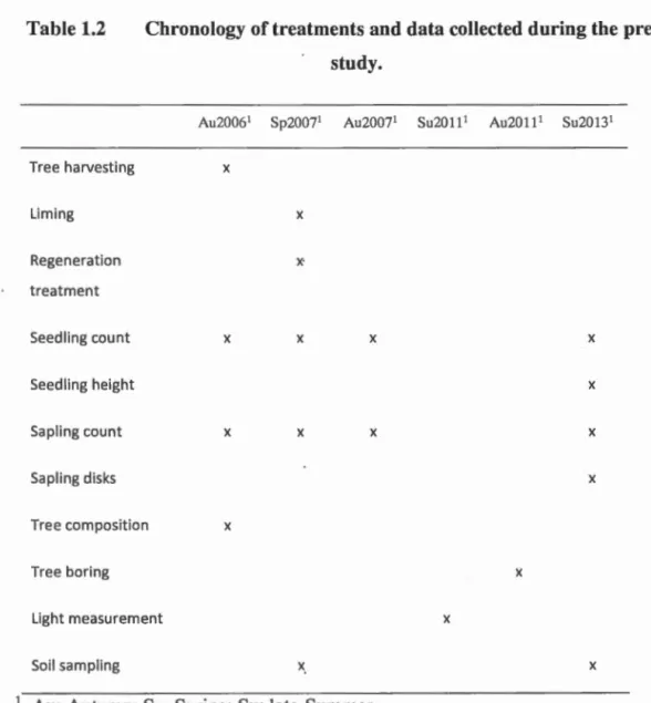
Table 1.2 Chronology of treatments and data collected during the present study. Tree harvesting Li ming Regeneration treatment Seedling cou nt Seedling height Sapling count Sapling disks Tree composition Tree boring
Light measurement
Soil sampling
Au20061 Sp20071 Au20071 Su20111 Au20111 Su20131 x x x· x x x x x x x x x x x x x x. x
1 Au: Autumn; Sp: Spring; Su: late-Summer
To quantify the light environment created by each canopy opening and beech regeneration treatment, we took hemispherical photographs (at 0.5 rn in height) at the centre of each treatment unit at the end of summer 2009. For each treatment unit, 5 soil
20
sam pies (one at each plot centre) were taken from the B-horizon in spring 2007 prior to liming and in summer 2013, and later composited to estima te average soi! conditions.
1.3.5 Laboratory analyses
The ring-widths of 12 years (1998-2009) for the tree cores, and 15 years (1998-2013) for the sapling disks were measured to the nearest 0.01 mm using a 40X magnification
scope and a sliding measurement stage (Velmex Inc., Bloomfield, NY, USA), which
was coupled to a digital meter. For light measurements, each hemispheric photograph was converted to black and white format and analyzed with GLA (Gap Light Analyzer; Fraser 1999). Finally, soils samples were air dried for severa! weeks and sieved to pass a 2 mm-mesh screen prior to analysis. Bulk pH of 2:1 (soil:deionized water) slurries was measured with a glass electrode-calomel probe (pHM82, Standard pH Meter; Radiometer Copenhagen, Bmnsh0j, Denmark). Exchangeable soil cations were
extracted with unbuffered 0.1 mol*L-1 BaCh solution (Hendershot et al. 1993). Cation
(Ca, Mg) concentrations were determined by atomic absorption spectrometry (PerkinElmer lnc., Wellesley, MA).
1.3.6 Data analyses
AJI of our statistical analyses followed the mode! comparison approach that was based
on the Kullback-Leibler information quantity, as presented by Anderson et al. (2000):
this approach is different from the classical nul! hypothesis testing approach as the goal is to identify the best mode! of a set of models rather than to test an alternative hypothesis vs a nul! hypothesis. For each response variable (indicator), we compared the performance of a full mode! to simpler models using the three factors (harvest intensity, liming and cleaning treatment) of our experimental design as predictor
variables. This approach allowed us to test various plausible hypotheses regarding the
effect of our predictor variables on the response variables in two ways. First, by
comparing the corrected Akaike information criterion (AICc) obtained by each mode!, it is possible to calcula te the weight ( m) of a specifie mode!, which can be interpreted
as the probability that this mode! is the best among ail tested models. Second, since a
predictor variable may appear in more than one mode!, it is also possible to sum up the
weight of the models in which a predictor variable appears. This cumulative weight
can be interpreted as the probability that a specifie predictor variable be part of the best tested mode! (in contrast with p values used in null mode! testing). Ali analyses were performed in R (version 3.1.0; R Development Core Team 2013) and were run
separately for SM and AB because the degrees-of-freedom for testing a four-way
interaction (with species as a factor) were too few.
For adult trees, we verified the effect of treatments on mean radial growth between the
post-harvest period (2007-2011) and the pre-harvest period (2002-2006) using a
mixed-effects mode!, with treatment unit as the random variable (lmer function of package lme4 in R). For saplings, the response to treatments was evaluated based on the difference in basal area between 2007 and 2013, summed by treatment unit, using
the lm function in R. We did not use 2006 data for saplings because we were more
interested in testing the treatment effects on post-harvest dynamics than in evaluating
direct harvesting effects. For the same reason, we used autumn 2007 data for AB (after destructive AB treatment), while we were able to use spring 2007 data for SM as they
were not destroyed during AB treatment. For saplings, we also verified the response in
mean sapling radial growth between the post-harvest period (2008-2013) and the pre-harvest period (2002-2006) using a mixed mode! in the same manner as we did for tree
growth. For seedlings, we first verified the treatment effects that were based on the
difference in the density (stems*ha-1
_1-22
treatment unit with the glm.nb function (MASS package in R). Second, we averaged the height of the tallest individual by species for each subplot and evaluated the effect of treatments using a mixed madel in the same manner as we did for tree growth. Finally, we compared the capacity of the 3 treatments to predict the species (response variable) that had the tallest seedling in subplots (in 2013) with a multinomiallogistic regression using treatment unit as a random variable; this analysis was performed with the polytomous package in R.
1.4 Results
1.4.1 Direct effects of treatments on light environment and sail chemistry
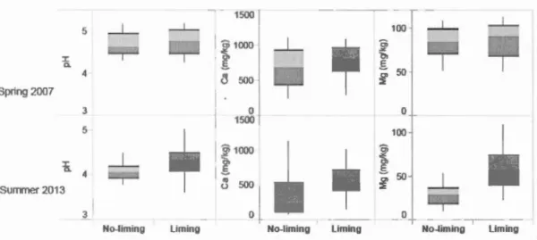
Clear-cutting greatly increased light availability compared to contrais and, to a lesser extent, to partial cuts (Figure 1.2). Beech sapling elimination also increased light availability, but not as much as clear-cutting. Madel comparisons showed that the additive madel including canopy opening alone or in combination with the beech elimination treatment bad respectively 73% and 27% probability of being the best madel to explain light availability when compared to the intercept madel (Table A.1). Seven (7) years after treatment, limed treatment units had higher Ca and Mg concentrations and slightly higher pH, while there were no marked differences in sail chemistry before treatment (Figure 1.3). For Ca and Mg, the madel using liming alone had more than a 99% probability of being better than the madel using the intercept alone while this probability dropped·to 75% for pH (Table A.1). Soil parameter values were generally higher, with or without liming, in 2006 than in 2013. We attribute this result to the season of sampling. In 2006, soil samples were taken in the early springbefore leaf emergence, while they were taken in late summer in 2013.
control selection eut clear-cut 70
1
60 501
~ ~ :ô 40 ro 'ai > ro :ë .2' 30 _J 2.0l_
10_j_
_ L _ r -0no beectl bee ch no lleech bee ch no beech bee ch
treatment treatment trealment treatment treatment treatment
Figm·e 1.2 Light availability as a function of canopy opening and beech sapling
elimination treatments. The limits of the box are the 25 and 75 percentiles, the
separa ting line between the two shades of grey is the median, the lower and
upper limits of the whiskers are the lOth and 90th percentiles, and points are
L 24 1500 5 _ j _ _ _ j _ 100 ; l1000 _L _ j _ 'ôi .>C :;:
"'
"'
a. .5..s
4a
Cl 50 500 :::E Spring 2007 3 0 0 1500 5_L
100~
_j_ ~ 10001
_L
î
~ 0, Cl 4 .5..s
50_j_
.,
Ol Summer 2013 u 500 :::E 3 0a
l
No-liming Liming No-limîng Li ming No-limîng Limîng
Figure 1.3 Effect of li ming on Ca and Mg concentrations and on pH.
Details of the box plots are included in Figure 1.2.
1.4.2 Mature tree radial growth
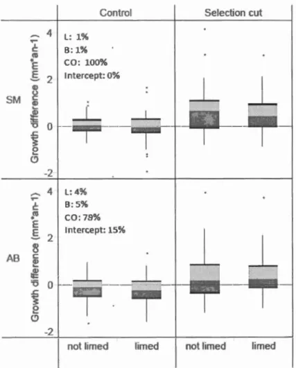
Mature tree radial growth of bath species increased from pre-treatment (2001-2006) to post-treatment period (2007-2011). Bath species reacted positively to selection cutting with canopy opening (CO) respective! y having 97% and 75% for SM and AB of being the best mode! that was tested (as indicated by w, Table 1.3). Since w is higher for SM than for AB, it means that the effect of the canopy opening treatment is statistically stronger for SM than for AB. However, since the intercept mode! is higher than 10 % (15%) for AB, it should not be complete! y rejected, meaning that there is still a reasonably high probability that none of our treatments (canopy opening, liming and
beech treatments) had an effect on
AB
tree radial growth (Figure 1.4, Table 1.3). WhileSM growth remained stable in contrais between the two periods, AB growth decreased. We attribute this decrease in tree growth to the sudden introduction of beech bark disease (nectria fungal infection caused by feeding injury from the exotic beech scale insect Cryptococcus fagisuga, e.g. Houston, 1975) into the area.
Control Selection eut ~ ,... 4 L: 1%
t
B: 1% ('Q È CO: lOO%g
2 lntercept: O% ID u SM c ID.!?
~_L
j_
"0 0 .s:::. ~ 0 .._ (.') -2 ,.... 4 L:4% ,... t B:S% ('Q C0:78%..
E lntercept: 15%s
2:s
AB c ID ...._l_
~ '5 0 .s:::. ~ 0 .._ (.') -2 1not limed limed
1
not limed limed
Figure 1.4 Mature tree radial growth change between pre and post treatment periods for sugar maple (SM) and American beech (AB) according to the canopy opening and timing ti·eatments. Percentages related to L, B, CO represent their
respective cumulative probabilities to be included in the best model (see
Methodology and Table 1.3 for details). The percentage associated with the intercept is provided fot· comparison. Details of the box plots are included in
26
1.4.3 Sapling basal area and radial growth
Basal area of sugar maple saplings (BAsM) decreased immediately following treatments because of the negative effects imposed by harvesting operations -for bath selection eut and clear-cut treatments -on sapling understory caver (Figure A.3). Post-treatment (2007 to 2013), none of the treatment had a clear effect on SM and AB sapling basal area (Table 1.3, Figure A.3). As was the case with mature tree radial growth, sapling growth of bath species increased after treatments (Figure 1.5). Again, it appeared that only opening the canopy (selection eut) had a positive effect on radial growth ( ro
=
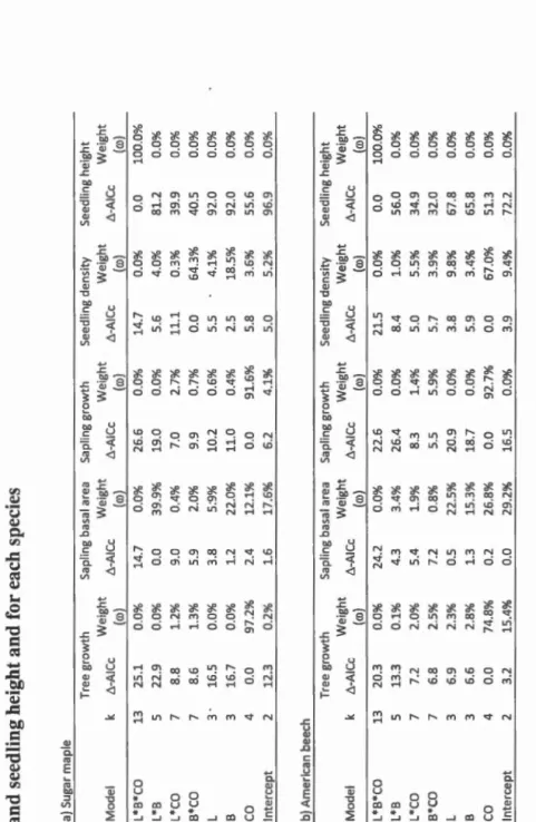
92 % for SM and 93 % for AB) and that liming had no effect ( ro < 1%, Table 1.3), even though growth variation among saplings appeared lower with liming. Further, the effect of canopy opening lasted longer for AB than for SM, given that six years after treatment AB sapling growth was still greater than its pre-treatment levet, white SM sapling growth returned to its pre-treatment level (results not shawn).Table 1.3 Model comparison for mature tree growth, sapling basal area, sapling radial growth, seedling density and seedling height and for each species a) Sugar ma p ie Tree growth Sapling ba s al a rea Sapling growth Seedl i ng den si ty Seedling height Mode! k t.-AICc Weight t.-AICc We ig ht t.-AICc We i ght 1'.-AICc Weight -Al Cc We ig ht ( w) ( w ) ( w ) ( w ) ( w ) L *B*CO 13 25 . 1 0 . 0 % 14 . 7 0 . 0 % 26 . 6 0 . 0% 14.7 0.0 % 0 . 0 100.0 % L *B 5 22.9 0 . 0 % 0 . 0 39 . 9 % 19 . 0 0 . 0 % 5 . 6 4.0 % 81.2 0 . 0% L*CO 7 8 . 8 1.2 % 9.0 0.4 % 7.0 2.7 % 11.1 0.3 % 39 . 9 0 . 0 % B * CO 7 8 . 6 1 . 3 % 5 .9 2 . 0 % 9 . 9 0.7 % 0 . 0 64.3 % 40.5 0 . 0 % L 3 • 16 . 5 0.0 % 3.8 5 : 9% 10.2 0 . 6 % 5.5 4.1 % 92 . 0 0 . 0 % B 3 16 . 7 0 . 0 % 1.2 22 . 0 % 11.0 0 . 4 % 2.5 18 . 5 % 92 . 0 0 . 0 % co 4 0 . 0 97.2 % 2 .4 12.1 % 0 . 0 91.6 % 5 . 8 3.6 % 55 . 6 0.0 % lntercept 2 12 . 3 0 . 2 % 1 . 6 17 . 6% 6 . 2 4 . 1 % 5.0 5.2 % 96 . 9 0 . 0% b) American beech Tree growth Sapling basal a rea Sap ling growth Seedling density Seedl i ng height Mode! 1'. -AICc Weight L'l-AI Cc Weight L'l-AI Cc Weight L'l-AI Cc We i ght L'l -AI Cc We i ght ( w ) ( w ) ( w ) ( w ) ( w ) L*B*CO 13 20 . 3 0 . 0 % 24 . 2 0 . 0 % 22 . 6 0 . 0 % 21.5 0 . 0% 0 . 0 100 . 0% L*B 5 13 . 3 0 . 1 % 4 . 3 3.4 % 26.4 0.0% 8.4 1.0% 56.0 0.0% L*CO 7 7 . 2 2 . 0% 5.4 1 . 9% 8 . 3 1.4% 5.0 5.5% 34 . 9 0 . 0% B*CO 7 6.8 2 . 5 % 7.2 0.8 % 5 . 5 5 . 9% 5 . 7 3 . 9% 32.0 0 . 0% L 3 6 . 9 2 . 3 % 0 . 5 22 . 5 % 20.9 0 . 0 % 3.8 9.8 % 67.8 0 . 0% B 3 6.6 2 . 8 % 1.3 15 . 3 % 18 . 7 0 . 0% 5.9 3.4 % 65.8 0 . 0% co 4 0.0 74.8 % 0 . 2 26 . 8 % 0 . 0 92 . 7 % 0.0 67 . 0% 51.3 0 . 0% lntercept 2 3 . 2 15 . 4 % 0 . 0 29.2 % 16.5 0 . 0 % 3 . 9 9.4 % 72.2 0 . 0% L: Liming; B : Beech sapling elimination treatment; CO: Canopy opening treatment ; k: number of parameters in the mod e l. t. -AIC c: Diff erence c o rr e ct e d Akaik e inform at i o n criteria compared wit h the b es t mode! ; w: m o d e ! weight.
2
8
Control Selection eut
2-L:3% ~ 8:1% ~ CO: 95%
1
'E 1-lnterœpt: 4%s
Q)o-
-
~
--
-.
_j_
~
-
rL.
1 0 SM c (!! _ _j ~ :0 .s:: ~ -1 -0 2-1
&! L: 1% .s:: 8: o%.
E 1- CO: lOO% _L_ .§. 1 ntercept: 0% el..J_
AB c 0--~ --Q)J:!
!>= '0 .s:: je
-1 -C>not limed lirned not limed limed
Figure 1.5 Sapling radial growth change between pre- and post-treatment
periods for sugat· maple (SM) and American beech (AB) according to the canopy opening and liming treatments. Percentages related to L, B, CO represent the
cumulative probabilities that liming, sapling beech elimination, and canopy opening treatments would be respectively included in the best model that was
tested for a species (see Methods and Table 1.3 for details). The percentage
associated with the intercept is provided for comparison. Details of the box plots
are included in Figure 1.2.
1.4.4 Seedling abundance and tallest height
The interaction between the beech control treatrnent and the canopy opening treatment provided the best madel ( ro
=
64%
,
Table 1.3) for explaining the development of sugarmaple seedling densities (DsM) from 2006 to 2013 (Figure 1.6). With a ro
=
19%,
the beech control treatment alone cannat be discarded, but liming and the canopy opening treatments, both with ro < 4 %, cannat be considered as appropriate models. More precisely, a clear increase in DsM was observed when the AB control treatment wasimposed, combined with no openings in the canopy. Otherwise, DsM was quite stable. The best madel for explaining AB density (DAs) development between 2006-2013 was clearly the one that included the canopy opening treatment alone (ro
=
67%
).
No other madel performed better than having a 10 % probability of being the best madel. Regardless of liming or beech control treatments, selection cuts led to an increase inDAB (Figure 1.6), while DAs did not change much for other canopy opening treatments.
For the tallest seedling indicator, the interaction between canopy opening, liming and
beech elimination treatments was the best mo del ( ro
=
100%,
Table 1.3) for bathspecies. The canopy opening treat~ent, as shawn by corrected Akaike information
criteria (AlCc) (in Table 1.3 and Figure 1.7), was the treatment that had the most
important effect on dominant seedling height. In the contrais, AB was clearly the
species with the dominant seedlings, even though dominant AB seedling height was
lower when there was an AB sapling elimination treatment. In selection cuts, AB was still the dominant species, even though dominant seedling height of SM was greater
Control SM Selection CUl Cl~ar-cut Control AB SelectJon eut Clear-cut OK
f
20K w-"~ a>' ~ g_ 10K .5l ~ 10K c w -"~ ,§ g_ SK ~ U) OK Figure 1.6 No Llmlng-No AB treatment ·1· l: 8% Llmlng Au-2006j_
6:87% co, 68% tntercept: 5% l =I
_L
_ L Su-2013 1 Au-2006 30l--
AB treatment Llmlng and AB treatmentDifference in seedling density before and after treatment according to the various treatments for sugar maple (SM) and American beech
(AB). Au: Autumn; Su: late-summer. Percentages related to L, B, CO represent
the cumulative probabilities that liming, sapling beech elimination, and canopy opening treatments would be respectively included in the best model that was
tested for a species (see Methods and Table 1.3 for details). The percentage
associated with the intercept is provided for comparison. Details of the box plots are included in Figure 1.2.
In clear-cuts, the height of dominant SM seedlings is very similar to that of AB dominant seedlings. The effects of liming and beech control treatments appeared to be