Science Arts & Métiers (SAM)
is an open access repository that collects the work of Arts et Métiers Institute of Technology researchers and makes it freely available over the web where possible.
This is an author-deposited version published in: https://sam.ensam.eu Handle ID: .http://hdl.handle.net/10985/14535
To cite this version :
Quentin COSSART, Frédéric COLAS, Xavier KESTELYN - Simplified converters models for the analysis and simulation of large transmission systems using 100% power electronics - In: 2018 20th European Conference on Power Electronics and Applications (EPE'18 ECCE Europe), Lettonie, 2018 - 2018 20th European Conference on Power Electronics and Applications (EPE'18 ECCE Europe) - 2018
Any correspondence concerning this service should be sent to the repository Administrator : [email protected]
Simplified converters models for the analysis and simulation of large
transmission systems using 100% power electronics
Quentin COSSART, Frédéric COLAS, Xavier KESTELYN
Univ. Lille, Arts et Metiers ParisTech, Centrale Lille, HEI, EA 2697-L2EP-Laboratoire d’Electrotechnique et d’Electronique de Puissance,
F-59000 Lille, France
E-Mail: [email protected]
Acknowledgements
This project has received funding from the European Union’s Horizon 2020 research and innovation programme under grant agreement No 691800. This paper reflects only the authors’ views and the European Commission is not responsible for any use that may be made of the information it contains.
Keywords
«Simulation», «Modelling», «Voltage Source Converter (VSC)», «Power transmission».
Abstract
In this paper, a model order reduction method is proposed, to simplify power electronics converters and allow simulating large transmission systems using 100% power electronics. Unlike existing methods it keeps the system’s physical structure, thus making the simulation and the analysis more flexible. This method is validated on a two-converter system and proves to be both conservative and accurate.
Introduction
The development of wind and solar photovoltaic power plants, as well as the multiplication of high voltage direct current links, increases the Power Electronics (PE) penetration in the transmission system.
As PE devices and Synchronous Generators (SG) have very different physical behaviors, the conditions to ensure the system stability are changing [1]. To cope with that, new converters controls need to be developed [2]. These controls have to be tested with numerical simulations as real-size experiments on transmission systems are impossible [3].
PE converters are complex systems, with many equations, variables and parameters. The aim of this work is to simulate and analyze large transmission systems with 100% PE [4]. In that case, using detailed converters models would lead to a high computation time and an arduous analysis. It is thus necessary to simplify the models of the converters [5]. This is called Model Order Reduction (MOR) in the literature.
Many MOR methods exist [6]. But despite being very accurate, most of them have an important drawback: by doing basis changes and truncations, they change the variables, the poles and the physical structure of the system, which is not flexible, as the stability analysis is not feasible anymore. In this paper, a structure-preserving MOR method, based on state residualization and modal analysis, is proposed and applied to a converter example. The obtained reduced model is then validated on a two-converter system to check if the important interactions between the converters are kept, even though the converters are reduced separately, and to verify that the reduced model is conservative. The first part of this paper describes the chosen converter, while the second one applies the MOR method to it and the third one is dedicated to the test case with two converters.
Grid Forming Converter model
General structure
In the case of a transmission system using 100% PE, the converters need to form the voltage waveform, just like would SG do. Theses converters are called grid forming converters [7].
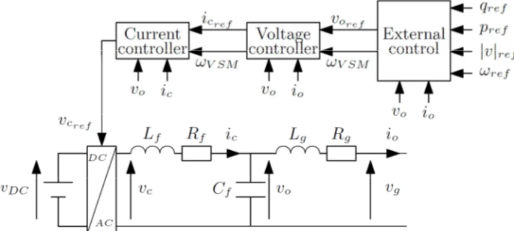
An example of grid forming converter is studied in this paper and then reduced. Its physical part is composed of the DC/AC converter itself connected to the infinite grid through an RLC filter and an RL line/transformer. Its control is made of an external loop, a voltage loop and a current loop.
The general structure of the converter is given in figure 1 but more details can be found in [8]. The different parts of the system are described in the next subsections.
Fig. 1 : General structure of the chosen grid forming converter External control
The external control is made of a Virtual Synchronous Machine (VSM) that mimics the behavior of a SG and a reactive power droop that gives the voltage reference for the voltage controller.
Their structures are given in figure 2 and 3, and their equations in (1)-(4).
Virtual synchronous machine
Fig. 2: Structure of the Virtual Synchronous Machine (VSM)
(1) !
"#$ (2)
In the rest of the paper, all the equations will be given in the dq reference frame of the VSM angle θVSM.
Reactive power droop
Fig. 3: Structure of the reactive power droop
* + +
(3)
, - |,| /*0+ + 1 (4)
Voltage controller
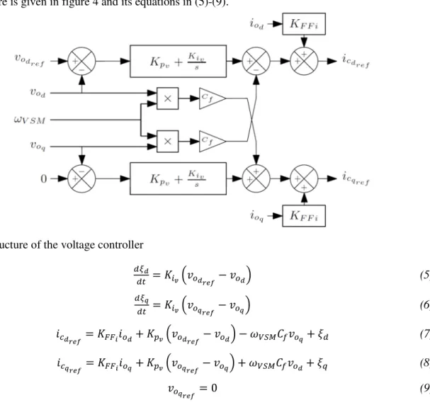
The voltage controller is made of two PI controllers. It gives the current reference to the current controller.
Its structure is given in figure 4 and its equations in (5)-(9).
Fig. 4: Structure of the voltage controller 2- 3 4 , - , - (5) 25 3 4 , 5 ,5 (6) 67- 38896 - 3: , - , - "#$; , 5 < (7) 675 38896 5 3: , 5 , 5 "#$; , - <* (8) , 5 0 (9) Current controller
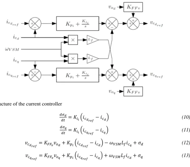
The current controller uses the output of the voltage controller as an input. This is called a cascaded loops structure. It is quite similar to the voltage control loop, with two PI controllers. It gives the voltage reference to the DC/AC converter.
Fig. 5: Structure of the current controller >- 3 49 67- 67- (10) >5 3 49 675 675 (11) ,7- 388, - 3:9 67- 67- "#$? 675 @ (12) ,75 388, 5 3:9 675 675 "#$? 67- @* (13) DC/AC Converter
To simplify, it is considered that the voltage of the DC/AC converter is equal to its reference. It is written in equations (14)-(15).
,7- ,7- (14)
,75 ,75 (15)
RLC filter
The RLC filter is described by equations (16)-(19). A 4 B-,7- , - C 67- "#$? 675 (16) A 4B5 ,75 , 5 C 675 "#$? 67- (17) D E-67- 6 - "#$; ,5 (18) D E5 6 75 6 5 "#$; , - (19) RL line/transformer
The RL line/transformer is described by equations (20)-(23). AF 4E- ,
AF 4E5 ,
5 , 5 C 6 5 "#$? 6 - (21)
, -6 - , 56 5 (22)
+ , 56 - , -6 5 (23)
Summary
To sum up, the converter is made of 13 differential and 10 algebraic equations (1)-(23). It is thus a 13th order system.
This model is simplified in the next part, using the developed structure-preserving MOR method.
Model order reduction of an example of grid-forming converter
General principle and participation factors
The first part of the proposed method is to linearize the equations (1)-(23). The algebraic equations are then injected into the differential equations to obtain a linear system represented using the state-space representation, like in (24).
∆H
H I∆J K∆L (24)
The main idea of the method is to freeze, in the nonlinear equations (1)-(23), the dynamics of the differential variables that influence the most the fastest poles of the linearized system (the eigenvalues of A that are far from the imaginary axis, see table I). This removes these fast poles while almost unchanging the slow ones, that are the most important for the stability analysis and the simulation. To do so, the participation factor [9] of each differential variable ∆JM in each eigenvalue N4 is computed. The participation factor is a dimensionless number between 0 and 1 that gives the participation (its influence) of each state variable in each mode of the system. It is defined in (25).
O4,M L4,MQ4,M (25)
In this equation, Q4,M is the R S entry of the 6 S right eigenvector of I associated to N4 and L4,M is the R S entry of the 6 S left eigenvector of I associated to N4.
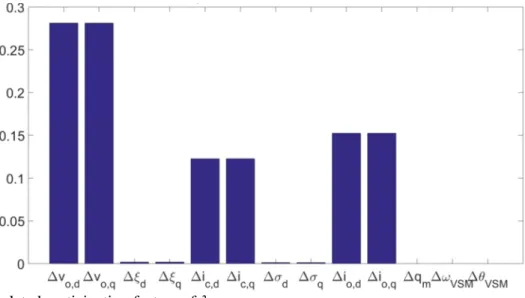
All the participation factors are calculated. An example for one particular double eigenvalue NT, U is given in figure 6. It shows that it is mainly influenced by the dynamics of the voltages and currents in the converter.
With the participation factors, it is then easy to know which variables influence the most an eigenvalue. As one state variable can participate in several eigenvalues and an eigenvalue can be influenced by several state variables, groups are formed in table I.
Table I: System eigenvalues and the state variables on which they depend
Eigenvalues State variables Model order
N V 1555 "#$ 12 N , Y 1048 \ 1796 NT, U 507 \ 32906 Na,b 430 \ 28496 , , , *, 6 , 6 *, 67 , 67* 6 Nc,d 31.76 \ 0.026 @ , @* 4 Ng 31.4 + 3 NY,V 1.03 \ 7.76 N 1 < , <*, h"#$ NA
Then to reduce the order of the model, the dynamics of the state variables that participate the most in the eigenvalue that one wants to remove are frozen. This is called state residualization [10]. According to table I, it is possible to derive a 12th order, a 6th order, a 4th order and a 3rd order model.
12th order model
To obtain the 12th order model, N V is removed by freezing the dynamic of "#$. (1) is changed into (26).
(26) As a differential equation is changed into an algebraic equation, the order of the model is reduced by one. The variables of the system are kept exactly the same, some dynamics are just frozen. This is flexible and it allows representing physically the reduced models with block diagram, just like for the full model, as can be seen in figure 7.
Fig. 7: Structure of the Virtual Synchronous Machine (VSM) after the reduction 6th order model
To obtain the 6th order model, (16)-(21) are changed into (27)-(32) to discard N , Y, NT, U and Na,b.
0 ,7- , - C 67- "#$? 675 (27) 0 ,75 , 5 C 675 "#$? 67- (28) 0 67- 6 - "#$; , 5 (29) 0 675 6 5 "#$; , - (30) 0 ,- , - C 6 - "#$? 6 5 (31) 0 , 5 , 5 C 6 5 "#$? 6 - (32)
4th order model
To obtain the 4th order model, (10)-(11) are changed into (33)-(34) to remove Nc,d.
Figure 8 shows how the current controller is modelled after the reduction. The physical structure of the converter is kept once again.
67- 67- (33)
675 675 (34)
Fig. 8: Structure of the current controller after the reduction 3th order model
Finally, to obtain the 3rd order model, (3) is changed into (35) to delete Ng. Figure 9 shows how the reactive power droop is modified by the reduction.
+ + (35)
Fig. 9: Structure of the reactive power droop after the reduction Pole comparison
To compare the models, it is interesting to look at the poles of the systems. Let’s consider the 3rd order reduced model (the most reduced one). In figure 10, the poles of the full (order 13) and reduced (order 3) systems turn out to be really close. The fast eigenvalues are removed, and the slow ones almost unchanged, just like wanted. It means that the stability is kept (no pole is deviated in the positive half-plane).
To validate this reduced model on larger systems, the study of a two-converter system is performed in the next section and time simulation are performed, as well as poles analysis.
Case study: reduced models of a two-converter system
The 3rd order reduced model is compared to the detailed model with the simulation of a two-converter system. As reduced models for each of the two converters are used (this is called a Cartesian approach. Each converter is modeled by a 3rd order model.) instead of a model reduction of the whole system (this is called a systemic or holistic approach), some interactions could be missed. Two fast
eigenvalues of two different converters could interact and create a slow (if not unstable) pole, which would be missed with the reduced models. This is investigated in this section.
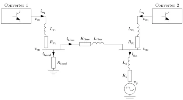
The considered system to be simulated is given in figure 11 and the parameters in table II. It is made of two grid-forming converters, separated by a transmission line, a load and the infinite grid.
Fig. 11: Structure of the studied two-converter system
Table II: System parameters in pu (converter 1; converter 2)
|,| ; |,| Y 1;1 ; Y 0.4; 0.1 + ; + Y 0; 0 C ; C Y 0.005; 0.007 ? ; ?Y 0.15; 0.17 ; ; ;Y 0.066; 0.07 C ; C Y 0.005; 0.007 ? ; ? Y 0.15; 0.17 j 314 rad/s 388k; 388l 1; 1 3:9k; 3:9l 0.65; 0.7 349k; 349l 20; 22 3889k; 3889l 0; 0 3:k; 3:l 1.79; 1.9 34 k; 34 l 81; 82 ; Y 3100; 3150 ; Y 2s; 2s k; l 1; 1 /* ; /*Y 0.000045; 0.000055 ; Y 31.42; 31.42 Cm 2.5 Cm4n 0.01 ?m4n 0.3 C 0.005 ? 0.15 , - 1 , 5 0
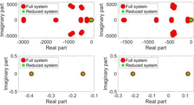
The idea of this study is to simulate a load increase after 1s. Two cases are considered: a stable case where Cm goes to 1.25pu and an unstable one, with an extreme load increase (or a short circuit), where Cm goes to 0.125pu. The aim is to check whether the reduced system is conservative or not (a stable full system gives a stable reduced system; an unstable full system gives an unstable reduced system).
On figure 12, the poles of the reduced and full systems for both cases are compared. The left side is for the stable case and the right one for the unstable case. The lower figures are a zoom on the two slowest poles of the system. This figure shows that the reduced model is conservative: when the full system is stable, the reduced one is stable too (and the same goes when unstable). Moreover, the poles that remain in the reduced system are really close to the slow poles of the full system. Only the fast poles are deleted.
Fig. 12: Pole comparison between the full and reduced models in the stable (left) and unstable (right) cases
In figure 13, the active power received by the grid is represented. The reduced and full models give similar results for both stable (left) and unstable (right) cases. By zooming in, it can be seen that just very fast transients are neglected while the general shape of the curve is the same, which shows the accuracy of the reduced models.
Fig. 13: Simulation comparison between the full and reduced models in the stable (left) and unstable (right) cases. Evolution of the active power received by the grid.
Conclusion
In this paper, a MOR reduction that preserves the physical structure of the system is proposed and applied to a PE converter. The obtained reduced model is then validated on a two-converter system to check if it is possible to reduce each converter separately while keeping a good accuracy. Two cases are tested, a stable and an unstable case. In both cases, the reduced model gives satisfying results by being accurate, conservative and by keeping the important interactions that can occur between the two converters. The slow poles of the system are kept almost unchanged and the fast ones are discarded. The time simulations show similar results in both full and reduced cases.
The next step will be to simulate a large system with reduced models and compare it to the case with detailed models, to generalize the outcomes of this study made on a small two-converter system. A work on the error estimation also has to be done to choose the most suitable model for each converter in the system depending on the events to be simulated and the system variables under consideration.
References
[1] J. Quintero, V. Vittal, G. T. Heydt, and H. Zhang, “The impact of increased penetration of converter control-based generators on power system modes of oscillation,” IEEE Trans. Power Syst., vol. 29, no. 5, pp. 2248–2256, Sep. 2014.
[2] J. Rocabert, A. Luna, F. Blaabjerg, and P. Rodríguez, “Control of Power Converters in AC Microgrids,”
IEEE Trans. Power Electron., vol. 27, no. 11, pp. 4734–4749, Nov. 2012.
[3] D. Ramasubramanian, V. Vittal, and J. M. Undrill, “Transient stability analysis of an all converter interfaced generation WECC system,” in 19th Power Systems Computation Conference, PSCC 2016, 2016, pp. 1–7.
[4] G. Denis, T. Prevost, M. Debry, F. Xavier, X. Guillaud, and A. Menze, “The Migrate project: the challenges of operating a transmission grid with only inverter-based generation. A grid-forming control improvement with transient current-limiting control,” IET Renew. Power Gener., 2017.
[5] Y. Gu, N. Bottrell, and T. C. Green, “Reduced-Order Models for Representing Converters in Power System Studies,” IEEE Trans. Power Electron., pp. 1–1, 2017.
[6] A. C. Antoulas, D. C. Sorensen, and S. Gugercin, “A survey of model reduction methods for large-scale systems,” Am. Math. Soc., vol. 280, pp. 1–28, 2006.
[7] J. M. Guerrero, M. Chandorkar, T. L. Lee, and P. C. Loh, “Advanced Control Architectures for
Intelligent Microgrids—Part I: Decentralized and Hierarchical Control,” IEEE Trans. Ind. Electron., vol. 60, no. 4, pp. 1254–1262, Apr. 2013.
[8] S. D’Arco, J. A. Suul, and O. B. Fosso, “Automatic Tuning of Cascaded Controllers for Power
Converters Using Eigenvalue Parametric Sensitivities,” IEEE Trans. Ind. Appl., vol. 51, no. 2, pp. 1743– 1753, Mar. 2015.
[9] I. J. Perez-Arriaga, G. C. Verghese, and F. C. Schweppe, “Selective Modal Analysis with Applications to Electric Power Systems, Part I: Heuristic Introduction,” IEEE Power Eng. Rev., vol. PER-2, no. 9, pp. 29–30, Sep. 1982.
[10] A. C. Antoulas, Approximation of Large-Scale Dynamical Systems. Society for Industrial and Applied Mathematics, 2005.