Prediction of necking in HCP sheet metals using a two-surface plasticity model

Science Arts & Métiers (SAM)

is an open access repository that collects the work of Arts et Métiers Institute of Technology researchers and makes it freely available over the web where possible.

This is an author-deposited version published in: https://sam.ensam.eu Handle ID: .http://hdl.handle.net/10985/18279

To cite this version :

Mohamed Yassine JEDIDI, Mohamed BEN BETTAIEB, Farid ABED-MERAIM, Mohamed Taoufik KHABOU, Anas BOUGUECHA, Mohamed HADDAR - Prediction of necking in HCP sheet metals using a twosurface plasticity model International Journal of Plasticity Vol. 128, p.102641 -2020

Any correspondence concerning this service should be sent to the repository Administrator : [email protected]

-1-

Prediction of necking in HCP sheet metals using a two-surface plasticity

model

M.Y. Jedidi1,3_{, M. Ben Bettaieb}1,2*_{, F. Abed-Meraim}1,2_{, M.T. Khabou}3_{, A. Bouguecha}3_{, M.} Haddar3

1_{Université de Lorraine, CNRS, Campus Arts et Métiers de Metz, LEM3, F-57000, France}

2_{DAMAS, Laboratory of Excellence on Design of Alloy Metals for low-mAss Structures, Université}

de Lorraine, France

3_{Laboratory of Mechanics, Modeling and Production (LA2MP), National School of Engineers of Sfax}

– Sfax – Tunisia

* _{Corresponding author: [email protected]}

Abstract

In the present contribution, a two-surface plasticity model is coupled with several diffuse and localized necking criteria to predict the ductility limits of hexagonal closed packed sheet metals. The plastic strain is considered, in this two-surface constitutive framework, as the result of both slip and twinning deformation modes. This leads to a description of the plastic anisotropy by two separate yield functions: the Barlat yield function to model plastic anisotropy due to slip deformation modes, and the Cazacu yield function to model plastic anisotropy due to twinning deformation modes. Actually, the proposed two-surface model offers an accurate prediction of the plastic anisotropy as well as the tension–compression yield asymmetry for the material response. Furthermore, the current model allows incorporating the effect of distortional hardening resulting from the evolution of plastic anisotropy and tension–compression yield asymmetry. Diffuse necking is predicted by the general bifurcation criterion. As to localized necking, it is determined by the Rice bifurcation criterion as well as by the Marciniak & Kuczynski imperfection approach. To apply both bifurcation criteria, the expression of the continuum tangent modulus associated with this constitutive framework is analytically derived. The set of equations resulting from the coupling between the Marciniak & Kuczynski approach and the constitutive relations is solved by developing an efficient implicit algorithm. The numerical implementation of the two-surface model is assessed and validated through a comparative study between our numerical predictions and several experimental results from the literature. A sensitivity study is presented to analyze the effect of some mechanical parameters on the

-2-

prediction of diffuse and localized necking in thin sheet metals made of HCP materials. The effect of distortional hardening on the onset of plastic instability is also investigated.

Keywords: two-surface plasticity model; hexagonal closed packed; plastic anisotropy; strength

asymmetry; plastic instability; forming limit diagram.

1. Introduction

Due to their interesting physical and mechanical properties, hexagonal closed packed (HCP) materials, such as titanium, magnesium and beryllium alloys, are widely used in aircraft, aerospace, automotive, computer and mobile device industries, as alternatives to conventional materials, such as steel or aluminum alloys. Indeed, HCP materials are characterized by their high tensile strength to density ratio (Li et al., 2017), high corrosion resistance (Lide, 2005), and high crack and fatigue resistance (Moiseyev, 2006). To better optimize the use of HCP materials in new industrial applications, their mechanical behavior should be accurately investigated. In this field, the modeling of physical mechanisms and modes that lead to plastic deformation and anisotropy in this class of materials has been getting growing attention from the scientific community (Cazacu and Barlat, 2004; Cazacu et al., 2006; Fan et al., 2018; Paramatmuni and Kanjarla, 2018; Kondori et al., 2019…). Several experimental investigations show that plastic deformation in HCP materials is mainly due to the activation of twinning and slip modes. These investigations also revealed that twinning mode results in tension–compression strength asymmetry, known as strength differential effect. Furthermore, the small number of slip systems in HCP materials (typically 3 to 6 slip systems versus 24 slip systems in BCC materials) leads to strong initial and evolving plastic anisotropy. In spite of the large number of works devoted to the study of their plastic anisotropy, experimental and theoretical investigations of HCP material ductility are still seldom, and often not very extensive (Chen and Hang, 2003; Chang et al., 2007; Lee et al., 2008; Steglich et Jeong, 2016). Though, during the design stage of a mechanical system, the forming capabilities of thin components are crucial to determine their behavior and service lifetime. In this context, a decision support tool that would provide relevant information from numerical prediction of formability limits should be developed. Towards this perspective, we have coupled an elaborate constitutive framework, which is capable of describing the evolution of the mechanical variables during deformation of HCP materials, with several plastic instability criteria. This coupling is used to predict the onset of diffuse and localized necking and to represent the predicted necking limit strains in terms of forming limit diagrams (FLDs).

 Constitutive modeling of HCP materials: to accurately model the mechanical behavior of HCP materials, several multiscale strategies have been set up in the literature (Lebensohn and Tomé, 1993; Kalidindi, 1998; Staroselsky and Anand, 1998; Wang et al., 2010; Wang et al., 2011; Song and Castañeda, 2018…). These multiscale schemes account for the above-mentioned peculiarities of the mechanical behavior of the studied materials (strong and evolving

-3-

plastic anisotropy and strength asymmetry), and hence offer good versatility to predict stress and strain anisotropy. Despite their undeniable advantages (physical foundations, accuracy, versatility…), the use of multiscale schemes is limited by the huge CPU time required by complex numerical applications, such as the prediction of the ductility limit, which is the primary concern of the current contribution. In fact, the CPU time required for the prediction of a complete FLD (i.e., strain paths ranging from uniaxial to equibiaxial tensile states), when using multiscale schemes for polycrystalline aggregates made of a few thousands of single crystals, ranges from days to weeks (Akpama et al., 2017; Gupta et al., 2018). To reduce the CPU time, it is more convenient to use phenomenological constitutive approaches instead of multiscale schemes in the modeling of the mechanical behavior of HCP polycrystalline materials. To this end, Cazacu and Barlat (2004) have developed an isotropic yield function to account for the asymmetry between tension and compression in the mechanical response. Some comparisons with results of polycrystalline simulations performed by Hosford and Allen (1973) reveal that the yield function proposed by Cazacu and Barlat (2004) describes very well the yielding asymmetry. The isotropic model developed in Cazacu and Barlat (2004) has been extended to plastic orthotropy in Cazacu et al. (2006). Known as CPB06, this extension takes into account the plastic orthotropy by introducing a linear transformation for the stress deviator tensor (through a transformation matrix). While it enables to reproduce with great accuracy the initial anisotropy of the studied materials, the CPB06 cannot accurately predict the evolving anisotropy due to the evolution of crystallographic texture. To better capture the evolution of plastic anisotropy and anisotropic hardening during loading, Plunkett et al. (2006) have developed an extension of the CPB06 model. In the latter investigation, the differential yield strengthening in compression and tension is described by predicting the components of the transformation matrix as well as strength differential parameters for different levels of plastic deformation. With this extension, a linear interpolation has been used to determine the evolution of these parameters. Another extension of the CPB06 model has been suggested by Plunkett et al. (2008). Instead of a single transformation, as introduced in CPB06, they used two independent linear transformations. It has been shown in Plunkett et al. (2008) that the accuracy in the description of the details of the plastic flow and anisotropy in both tension and compression can be further increased if more than two linear transformations were included in the formulation. The Cazacu models and their subsequent extensions have been widely used to model the mechanical behavior of various HCP materials and alloys. For instance, good correlations were observed between experimental results and numerical predictions obtained by Cazacu’s models for the mechanical behavior of HCP materials, such as high-purity α-titanium (Nixon et al., 2010), and titanium alloy Ti-6Al-4V (Gilles et al., 2011; Khan et al., 2012). The Cazacu anisotropic functions have also been used to model plastic anisotropy of magnesium alloys, such as AZ31 alloy (Muhammed et al., 2015; Soare et al., 2016), and ZEK100 alloy

-4-

(Muhammed et al., 2015; Abedini et al., 2017). Despite the relevance of the Cazacu models in the description of plastic anisotropy and strength asymmetry of HCP materials, a number of investigators suggested using more elaborate plasticity models. Indeed, the coexistence of slip and twinning modes leads to complex physical mechanisms causing a significant change in the shape of the yield surface with accumulated plastic deformation, which cannot be described by traditional single yield surface. In elaborate plasticity models, plastic anisotropy resulting from slip and that induced by twinning modes are treated separately by two yield functions: a symmetric yield function to model the slip mode, and an asymmetric yield function representing twinning-dominated flow. The two-surface modeling concept has been introduced in Mróz (1967) and Krieg (1975). This concept has recently been applied in Lee et al. (2008) to model the mechanical behavior of HCP materials, especially AZ31 magnesium alloy sheets. In the latter model, each surface is defined by the Drucker-Prager yield function, suitably modified to account for the anisotropy of magnesium alloy sheets. The same concept has been used by Kim et al. (2013) to model temperature dependent anisotropic/asymmetric plastic behavior of AZ31 magnesium alloy sheets, where the Hill’48 (resp. CPB06) yield function has been used to model the slip (resp. twinning) dominant mode. More recently, Steglich et al. (2016) have used a two-surface approach to model the evolution of plastic anisotropy in rolled thin sheets made of two different rolled magnesium alloys (AZ31 and ZE10). In the latter contribution, the Barlat (Barlat, 1991) and the CPB06 yield functions have been employed to model plastic anisotropy due to slip and twinning modes, respectively. Following this study, Madi et al. (2017) have developed an identification strategy, which includes specimens along the plate principal directions and off-axes specimens along diagonal orientations in principal planes, and this strategy has been extended by Kondori et al. (2019) to model plastic anisotropy in thick plates (3D modeling). The constitutive framework developed in Steglich et al. (2016), Madi et al. (2017) and Kondori et al. (2019) is used in the current contribution after its extension to incorporate the effect of distortional hardening on the macroscopic behavior. In fact, it is well known that for HCP materials, the twinning activity is gradually exhausted and the asymmetry decreases or even reverses (Lou et al., 2007; Kondori and Benzerga, 2014). This behavior cannot be captured using constant anisotropy coefficients, as it is the case in the original model developed in Steglich et al. (2016), Madi et al. (2017) and Kondori et al. (2019). An attempt to remedy this limitation in the context of HCP sheet alloys has recently been proposed by Yoon et al. (2013), who considered that the anisotropy coefficients are dependent on the effective plastic strain. The approach proposed by Yoon et al. (2013) has been followed by other authors to accurately model the distortional hardening resulting from the effect of the evolution of the anisotropy parameters on the macroscopic mechanical response (Ghaffari Tari et al., 2014; Muhammad et al., 2015; Lee et al., 2017). This choice is motivated by the capabilities and versatility of this modeling approach, which have been proven by the comparison between

-5-

experimental results and numerical predictions for a large variety of mechanical tests. The developed framework is based on a finite strain rate-independent formulation, with an associative flow rule and a plastic strain rate assumed to be normal to the activated yield functions. To numerically integrate the constitutive equations governing this model, we have developed an implicit integration scheme, which allows us to robustly switch from one active deformation mode to another. The accuracy and the efficiency of the developed numerical scheme are checked through several numerical results. The numerical predictions are assessed and validated by comparison with reference results taken from the literature (e.g., Steglich et al., 2016).

 Plastic instability prediction: during sheet metal forming processes, plastic deformation is often limited by the occurrence of plastic instability. To predict the onset of the latter and represent the corresponding necking limit strains in the form of FLDs, several plastic instability criteria have been developed in the literature. One of the most well-established and theoretically-sound criteria is the bifurcation approach initially proposed by Hill (1952). In the current contribution, the general bifurcation criterion (Drucker, 1950, 1956; Hill, 1958) has been used to predict the occurrence of diffuse necking in HCP thin sheets. This criterion will be called GBC in what follows. As to localized necking, it is predicted by another bifurcation criterion, based on the condition of loss of ellipticity of the governing equations (Rudnicki and Rice, 1975; Rice, 1976). This strain localization criterion, shortly denoted as RBC in what follows, is generally capable of predicting strain localization at realistic (finite) limit strains in the range of positive strain-path ratios when the constitutive framework exhibits some destabilizing effects, such as the development of vertices at the current points of the yield surface. Despite the development of vertex points when both slip and twinning modes are activated, it is shown in the present contribution that, within this particular two-surface plastic anisotropy constitutive framework, the Rice bifurcation criterion does not predict localized necking at realistic (finite) limit strains in the range of positive strain-path ratios. To overcome this limitation, the initial imperfection approach, developed by Marciniak and Kuczynski (1967) and briefly called hereafter M–K approach, is adopted. For HCP materials, this approach has been coupled with a limited number of constitutive frameworks to predict the onset of plastic strain localization. For instance, Lévesque et al. (2016) have recently used a rate-dependent multiscale scheme based on the Taylor model to predict the occurrence of strain localization in magnesium alloys. With regard to phenomenological approaches, an extension of the CPB06 model, developed by Plunkett et al. (2006), has been coupled in Wu et al. (2015) with the M–K approach to predict forming limit diagrams for materials with HCP structure. However, the current contribution represents the first time that bifurcation criteria are applied for the prediction of diffuse and localized necking in HCP materials. The application of these criteria requires the analytical expression of the continuum tangent modulus to be determined. The

-6-

derivation of such an elastoplastic tangent modulus is detailed in the present contribution. The coupling of the initial imperfection approach with the elastoplastic constitutive framework may be mathematically formulated as a strongly non-linear twenty-equation system (with twenty unknowns). We have developed an implicit algorithm to solve this set of equations. The adopted instability criteria are implemented using the multi-paradigm numerical computing environment

Mathematica. Note that the developed prediction approaches are sufficiently general to be

applied for the determination of necking in a wide range of HCP alloys. In the current investigation, these approaches are used to predict the formability limit of thin sheets made of magnesium alloy AZ31. This choice is motivated by the growing use of this well-known alloy in several industrial applications (automotive and aircraft industries) and by the availability of identified material parameters for this alloy in the literature (Steglich et al., 2016; Kondori et al., 2019). A sensitivity study is also conducted to analyze the effect of some material parameters on the predicted limit strains. Furthermore, the effect of distortional hardening on the onset of plastic instability is investigated.

A brief outline of the present paper is as follows:

 Section 2 details the constitutive framework selected to model the mechanical behavior of HCP materials as well as the main equations governing the adopted necking criteria.

 Section 3 outlines the numerical implementation of the constitutive equations coupled with the instability criteria presented in Section 2.

 Section 4 addresses the validation of the developed model and presents a numerical investigation to analyze the sensitivity of the predicted ductility limits to various material parameters.

 Section 5 closes our contribution by some conclusions and future work.

2. Theoretical framework

In this section, the main equations that describe the two-surface constitutive framework are presented. Then, the expression of the analytical tangent modulus is derived from these constitutive equations. This elastoplastic tangent modulus is required in the mathematical formulation of the necking criteria presented at the end of this section.

2.1. Constitutive equations

The constitutive modeling adopted in the current investigation is taken to be rate-independent and is formulated in the finite strain range. As a departure point of the theoretical framework developed in the subsequent sections, the spatial velocity gradient g is additively decomposed into its symmetric and skew-symmetric part, denoted d and w, respectively:

-7-

g   d w (1)

To satisfy the objectivity principle (i.e., frame invariance), objective derivatives for tensor variables should be used (Sidoroff and Dogui, 2001). A practical approach, adopted to ensure frame invariance while maintaining simple forms for the constitutive equations, consists in reformulating these equations in terms of rotation-compensated variables. In the present work, a co-rotational approach based on the Jaumann objective rate is used. Hence, tensor quantities are expressed in a rotating frame, so that simple material time derivatives can be used in the constitutive equations. The rotation r, which defines this rotating frame with respect to the fixed one, is derived from the spin tensor w

(skew-symmetric part of g) through the following relation:

.

,

r r

T



w

(2) with rT _{is the transpose of tensor r.}

In the remainder of Section 2.1, all tensor variables will be expressed in the rotating frame (called co-rotational frame), that is to say, using rotation-compensated variables. Consequently, time derivatives are involved in the constitutive equations, making them identical in form to a small-strain formulation. The strain rate d is itself split into its elastic part de _{and plastic part d}p_:

d de dp

(3) The stress rate is described with a hypoelastic law:

:

C d

 e e

 (4)

where Ce _{denotes the fourth-order elasticity tensor. Here, elasticity is assumed to be isotropic and is}

defined by two material parameters: the Young modulus E and the Poisson ratio .

The plastic strain rate dp _{is assumed to result from a contribution due to slip-dominated deformation}

mode, denoted dp s

, and a contribution induced by twinning-affected deformation mode, designated as

dp t _{(Steglich et al., 2016; Kondori et al., 2019):}

dp dp s dp t ₍₅₎

Both dp s _{and d}p t _{are given by an associative plastic flow rule (normality law):}

, d    d     s t p s



s



p t



t



  (6) where:

 s _(resp. t_{) represents the slip (resp. twinning) yield function and is equal to} s_Rs _(resp.

 t t R  ),  s (resp. t

) is the equivalent slip (resp. twinning) strain rate (also called the plastic multiplier),  s _(resp. t_{) stands for the equivalent slip (resp. twinning) stress,}

-8-

 s

R (resp. t

R ) denotes the slip (resp. twinning) yield stress. In the current contribution, both self-hardening (i.e., the effect of the plastic strain of a deformation mode to increase the yield stress of the same mode) and latent hardening (i.e., the effect of the plastic strain of a deformation mode to increase the yield stress of the other mode) are considered. Hence, _Rs _and

t

R are defined by the following generic forms:



 ,



,



 ,



.

s s s t t t s t

R R R R (7)

It has been shown in several previous contributions that slip-induced plasticity is almost insensitive to the stress sign (i.e., the tensile and compressive stresses required for the activation of the slip mode are equal in absolute value). Furthermore, the small number of slip systems in HCP materials leads to a strong evolution of crystallographic texture, and hence, of plastic anisotropy. According to Steglich et al. (2016) and Kondori et al. (2019), the specific characteristics of tension/compression asymmetry and strong evolution of plastic anisotropy are accurately accounted for by the anisotropic yield function developed by Barlat et al. (1991) and briefly called BLB91. In the BLB91 model, the equivalent slip stress s _{is defined by the following expression:}





1 1 2 2 3 1 3 1 2 /   _      _    s s s s a a a a s s s s s s s















(8)

In the above equation,



1

s

,



2

s

and



3

s

are the eigenvalues of a tensor s ₍

1  2  3

s s s







), which is obtained from the Cauchy stress tensor  by the following linear transformation:





,

s  _{L Τ}s 

  (9)

where Ls _{is a fourth-order transformation tensor defined in a matrix form as follows:}

11 12 13 12 22 23 13 23 33 44 55 66 0 0 0 0 0 0 0 0 0 0 0 0 0 0 0 0 0 0 0 0 0 0 0 0 L                     s s s s s s s s s s s s s l l l l l l l l l l l l (10)

and matrix Τ is given by:

2 1 1 0 0 0 1 2 1 0 0 0 1 1 2 0 0 0 1 3 0 0 0 3 0 0 0 0 0 0 3 0 0 0 0 0 0 3 T     _{ }        _{ }         (11)

-9-

The plastic deformation behavior of HCP materials is characterized by the yielding asymmetry of the stress state between tension and compression. This asymmetry is due to the activation of the twining deformation mode. To accurately capture the effect of this asymmetry on the shape of the anisotropic yield function, we have used the CPB06 yield criterion (Cazacu et al., 2006) to compute the equivalent twinning stress t_{, which is defined by the following expression:}



 

 







1 1 1 2 2 3 3 /        t t t t a a a a t t _k t t _k t t _k t        (12)

where k is a material parameter that describes the asymmetry degree of the deformation behavior, while



₁t_, 2



t _and 3



t _(with 1  2  3 t t t







) are the eigenvalues of a tensor t _{related to  by:}



L Τ



   

t t

  (13)

The orthotropic transformation matrix Lt _{is defined by the following expression:}

11 12 13 12 22 23 13 23 33 44 55 66 0 0 0 0 0 0 0 0 0 0 0 0 0 0 0 0 0 0 0 0 0 0 0 0 L         _{ }           t t t t t t t t t t t t t l l l l l l l l l l l l (14)

The material parameters ( a , k, l ) involved in Eqs. (8), (10), (12) and (14) are classically identified on the basis of a set of mechanical tests (uniaxial tension, uniaxial compression, simple shear…). An experimental methodology developed to identify these parameters has been presented and extensively discussed in Steglich et al. (2016) and Kondori et al. (2019).

The plastic flow may occur by activating one of the two plastic deformation modes (slip or twinning) or both modes simultaneously. The activation of each deformation mode is governed by the following Kuhn–Tucker constraints: slip mode: ) 0 0 0 twinning mode: ) 0 0 0. s s s s s s t t t t t t R R                            (15)

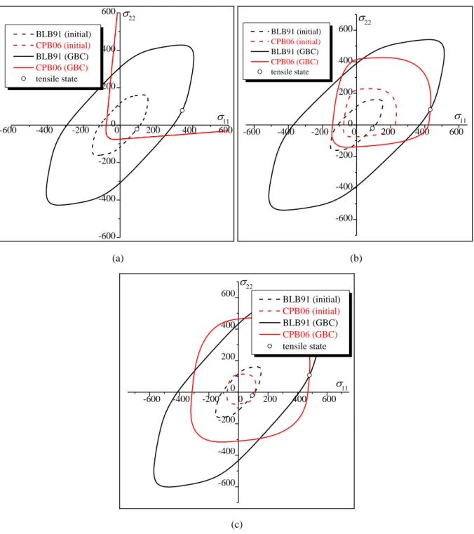
The possible scenarios for the activation of the different deformation modes are illustrated in Fig. 1, where the distinct yield surfaces are plotted in the 1122 space normalized by the initial slip yield

-10-

-1 0 1 2 -1 0 1 CPB06 BLB91 __ __ stress state -1 0 1 2 -1 0 1 CPB06 BLB91 __ __ stress state (a) (b) -1 0 1 2 -1 0 1 CPB06 BLB91 __ __ stress state (c)

Fig. 1. Possible scenarios for the activation of the different deformation modes: (a) Slip mode only; (b) Twinning mode only; (c) Slip and twinning modes simultaneously.

Note that if the anisotropy transformation matrices Ls _{and L}t _{and the strength differential parameter} k are taken to be constant, Eqs. (15) describe isotropic hardening, i.e. a proportional expansion of the two yield surfaces, without any shape change. To accurately account for the effect of the rapid change of plastic anisotropy in the modeling of the mechanical behavior, we assume that the different anisotropy parameters (i.e., the components of matrices Ls _{and L}t _{and parameter}

k) are dependent on the equivalent slip and twinning strains s and t:



,



,



,



,



,



.

-11-

The consideration of the evolution of the anisotropy parameters during plastic loading allows incorporating the effect of distortional hardening, in addition to isotropic hardening, on the macroscopic response (Yoon et al., 2013; Ghaffari Tari et al., 2014; Muhammad et al., 2015; Lee et al., 2017).

The Kuhn–Tucker constraints given by Eq. (15) (two inequalities and one equality for each deformation mode) can be equivalently expressed as a single equality by using the Fischer–Burmeister equality (Fischer, 1992; Fischer, 1997):

    



    



2 2 2 2 slip mode: 0 twinning mode: 0             s s s s s t t t t t





















(17)

The Fischer–Burmeister form is more convenient for the numerical implementation of the consistency condition. For instance, the Fischer–Burmeister form has been used in Akpama et al. (2016), instead of the classical formulation given by Eq. (15), in order to compute the slip rates within a rate-independent crystal plasticity constitutive framework. Adopting this compact form allows avoiding the recourse to the traditional elastic prediction–plastic correction algorithm, generally used to integrate rate-independent constitutive equations. Indeed, the use of the conventional form of the Kuhn–Tucker constraints may lead to some numerical difficulties when several deformation modes (more than one) are simultaneously or separately activated. These difficulties are related to the robust switch from one deformation mode to another. Hence, in the current work, Eq. (17) has been used to build the numerical scheme for the integration of the constitutive equations.

The specific expressions for the evolution laws of the components of the anisotropy parameters (i.e., the components of matrices Ls _{and L}t _{and parameter}

k) as well as the hardening yield functions s

R

and t

R will be provided in Section 4.

2.2. Analytic computation of the continuum tangent modulus

The constitutive framework described in Section 2.1 is complemented here by the derivation of the expression of the analytical tangent modulus , which is essential for the subsequent developments related to the analysis of diffuse and localized necking. This tangent modulus relates the nominal stress rate n to the velocity gradient g, as expressed by the following relation:

: . 

n _g (18)

To derive the expression of , let us first recall the relationship between the Cauchy stress tensor  and the nominal stress tensor n:

1_{. ,} j 



n f  (19)

where f is the deformation gradient and j its determinant. By taking the time derivative of Eq. (19), one obtains:

-12-

 





1 . Tr . nj f   d g  (20)

In the current investigation, an updated Lagrangian approach is adopted. Accordingly, f is set to the second-order identity tensor I2 and j is set to 1. Hence, Eq. (20) reduces to:

 

Tr .

n   d g (21)

Using Eq. (1) and the Jaumann derivative of the Cauchy stress tensor , Eq (21) can be rewritten in the following form after some straightforward developments (Haddag et al., 2009):

 

Tr . .

n C e de  d d  w

. (22)

To derive a constitutive relation expressed in the form of Eq. (18), each of the terms on the right-hand side of Eq. (22) is conveniently rewritten so as to obtain the following relations:

 

_

_





1 1 2 2 3 ₃ Tr 1 , with 2 . 1 . 2 C d C g d C g d C g w C g  _     _  _{  }   _{ }        _{ }   _  

 

 

 

 

 

e e ep ijkl ij kl ijkl jl ik jk il ijkl ik jl il jk C C C    , (23)

where _kl is the Kronecker delta.

The analytical tangent modulus is finally derived by combining Eqs. (22) and (23):

1 2 3

C C C C

 ep   

. (24)

In what follows, we provide in some details the computation of the elastoplastic tangent modulus Cep

. In the subsequent developments, we assume that the two deformation modes (namely slip and twining) are simultaneously activated. The special case when only one deformation mode is activated is addressed at the end of this section.

The elastoplastic tangent modulus Cep

is defined as follows:





: : : e e e p s p t ep ep C d C dd d C dC g  _. (25)

As the two deformation modes are activated, the Kuhn–Tucker conditions given by Eq. (15) are written in their rate forms:

slip mode: 0, twinning mode: 0, V V













              s s ss s st t t t ts s tt t M M M M (26) where: , , , , , . V V





















                      s s s s ss st s t t t t t ts tt s t M M M M (27)

-13-

The expressions of s /_, t _/_{, M}ss_{, M}st_{, M}ts _{and M}tt _{are given in Appendix A.}

By combining Eqs. (3)-(6), one can obtain the following expression for the stress rate :





: C d V V  e 



s s



t t    _. (28)

Using Eqs. (27) and (28), Eq. (26) can be reformulated as:





, :  V C : d V   0, , ,















    e    

s t M s t (29)

which can be expressed in a more compact matrix form:

A  Y_, (30) where: : : : , , . : : : V C d V C V V C V Y A V C V V C V V C d





                      _{ } _{ } _{ }            s e s e s ss s e t st s t e s ts t e t tt t e t M M M M (31)

Hence, the components of vector  can be determined by solving Eq. (30):





, : V :C : ,d , ,

 

_

_

    e

_



s t Β  s t (32)

where  is the inverse of matrix A .

Substituting vector  into Eq. (28) allows the following expression for  to be obtained:







e e :



: , , with : e, , s t s t.   

_

 

_

 C  C V X d   X  V C   (33)

The comparison between Eq. (25) and Eq. (33) allows identifying the expression of the elastoplastic tangent modulus Cep :



:



, , Cep Ce  Ce V X   s t.  (34)

When the mechanical behavior is purely elastic (neither of the deformation modes is activated), Eq. (34) reduces to:

Cep Ce

. (35)

In case where only one deformation mode is activated, Eq. (34) reduces to the following expression:



 





 



: : slip mode : , : : : : twinning mode : . : : C V V C C C V C V C V V C C C V C V                 e s s e ep e s e s ss e t t e ep e t e t tt M M (36)

Once determined, the expression of the elastoplastic tangent modulus Cep

is introduced in Eq. (24) to compute the analytical tangent modulus .

-14-

2.3. Necking criteria

2.3.1. General plane-stress state

An orthogonal Cartesian coordinate system



x x x1, 2, 3



is defined, where axes x x1, 2 and x3 coincide

with the rolling (L), transverse (T), and normal (S) directions of the sheet, respectively. To predict the necking limit strains, we consider a quasi-static deformation of a thin HCP sheet submitted to in-plane biaxial loading in the plane



x x1, 2



. Considering the small thickness of the sheet, and following most

studies on sheet metal formability, a generalized plane-stress state is assumed (Hutchinson et al., 1978a). With this assumption, the out-of-plane components of the Cauchy stress tensor are equal to zero, namely:

3 13 23 33 0

x

     

 







_. (37)

The metal sheet is taken to be initially stress-free. Hence, the plane-stress conditions can be expressed in terms of the components of the nominal stress rate:

13  31  23  32  33 0

n n n n n _. (38)

Eq. (38) also implies that the out-of-plane components of the velocity gradient g are equal to zero:

13  31  23  32 0

g g g g _. (39)

The general constitutive equation (18) can be expressed under the plane-stress conditions as follows (Akpama et al., 2017): : n g_, (40) where: 11 12 11 12 21 22 21 22 , , , , : . n g        _{ } _{ }                   n n g g n n g g (41)

2.3.2. Bifurcation criteria

Diffuse necking is predicted here by the general bifurcation criterion (GBC). This criterion states that plastic instability occurs when the second-order work vanishes (Drucker, 1950, 1956; Hill, 1958). To mathematically formulate this criterion, let us introduce the tangent modulus p _{relating the rate of}

the in-plane first Piola–Kirchhoff stress p to the rate of the in-plane deformation gradient f :

_p p:_f

. (42)

The tangent modulus p _{is obtained from the analytical tangent modulus introduced in Eq. (40) by}

-15-

, , , 1, 2 :

  p 

ijkl jikl

i j k l _. (43)

According to the GBC, diffuse necking is predicted when at least one eigenvalue of the symmetric part of p _{(called hereafter} p

sym) becomes negative (Bouktir et al., 2018).

The bifurcation theory has also been used to derive a localized necking criterion. This material instability approach, initially developed by Rudnicki and Rice (1975) and Rice (1976), states that plastic strain localization occurs when the determinant of the acoustic tensor vanishes. This Rice bifurcation criterion (RBC) is mathematically expressed by the following equation:





det v. .v 0_, (44)

where v is the unit vector normal to the localization band and lying in the plane



x x1, 2



. In the

frame



x x1, 2



, vector v is given by the following components



cossin



(with

90

 



 ). Further details about the Rice bifurcation approach can be found in Ben Bettaieb and Abed-Meraim (2015).

2.3.3. Initial imperfection approach

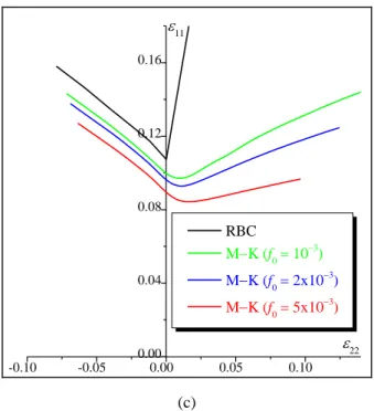
The occurrence of localized necking is also predicted by using the imperfection approach, initially proposed by Marciniak and Kuczynski (1967). The initial version of this approach has been restricted to the prediction of the formability limits in the range of positive strain-path ratios (between the plane-strain tension state and the equibiaxial tension state). Its extension to the range of negative plane-strain-path ratios has been developed by Hutchinson et al. (1978b). Hereafter, the extended form of the initial imperfection approach (M–K theory) will be used. The M–K analysis is based on the assumption of the preexistence of an initial geometric imperfection, in the form of a narrow band across the thickness of the metal sheet, as shown in Fig. 2.

(a) (b)

Fig. 2. Initial imperfection approach: (a) Configuration before loading; (b) Configuration after loading.

-16-

 The kinematic compatibility condition between the band zone (designated as ‘B’) and the homogeneous zone (designated as ‘H’). This condition allows linking the in-plane velocity gradient in the band zone gB _{to its counterpart in the homogeneous zone g}H_{, through a jump}

vector c and vector v normal to the band:

gB gH  c v

. (45)

 The force equilibrium across the interface between the band and the homogeneous zone:

. .

v n v n

 B H

, (46)

where  is the relative thickness of the band zone, which is equal to the ratio eB /eH_{. Here e}B

(resp. eH_{) is the current thickness of the band zone (resp. the homogeneous zone).}

 The plane-stress constitutive framework both in the band and in the homogeneous zone:

: ; :

nB  B gB nH  H gH

. (47)

The combination of equations (45), (46) and (47)) allows the following expression for the jump vector

c to be obtained:





1









. . . :

c v B v  v H  B gH

. (48)

Equations (45)–(47) are supplemented by the following two evolution equations:

 The evolution of the relative thickness of the band zone  as a function of its initial value 0

and the strain components normal to the plane of the sheet ₃₃B _and

33 H_:  33 33 0       B H e _. (49)

 The evolution of the band orientation, defined by vector v



cos

 

 sin

 





, as a function of its initial value ₀ and the strain components ₁₁H _and

22 H  :

 

 11 22 0     _   _





H H arctan tan e _. (50)

3. Algorithmic aspects

3.1. Bifurcation criteria

To predict the onset of necking using both bifurcation criteria, and to plot the corresponding necking limit strains in terms of forming limit diagrams (FLDs), the metal sheet is submitted to biaxial loading defined by the following form of velocity gradient g:

11 11 33 0 0 0 0 0 0 g d             d d d



_, (51)

-17-

where:

- d is the major strain rate, which is set here to 1 all along loading. As the behavior is rate-11

independent, the value given to d has no effect on the mechanical response. ₁₁

-  is the strain-path ratio, which ranges from 1 2/ (uniaxial tension state) to 1 (equibiaxial tension state).

- the component d is a priori unknown and is determined from the plane-stress condition ₃₃

(₃₃ 0).

The algorithm developed for the prediction of forming limit diagrams using both bifurcation criteria is based on two nested loops:

 For each strain-path ratio



ranging between 1 2/ and 1 (with



 ):

 For each time increment [ ,t t_{n n1}] (with t_n1 t_n t), we apply the incremental algorithm detailed in Section 3.3 to integrate the constitutive equations and then to compute the analytical tangent modulus . Once is computed, the condensed moduli and p _are

determined by Eqs. (41) and (43), respectively. To apply the general bifurcation criterion, the eigenvalues of p

sym (symmetric part of

p_{) are computed. Diffuse necking is predicted}

when the smallest eigenvalue of p

sym vanishes or, in an equivalent way, when p sym

becomes singular (as p

sym is positive definite before it becomes singular). To apply the

Rice bifurcation criterion, the orientation



providing the minimum value for





det v. .v over the interval



0 ,90 



is searched. If this minimum value is negative, localized necking is predicted and the computation is stopped. As long as the conditions for necking are not met yet, the different mechanical variables are updated and the computation is continued for the next time increment.

3.2. Initial imperfection approach

When the initial imperfection approach is followed, the homogeneous zone of the sheet is submitted to the same loading as that prescribed for the whole sheet in Section 3.1. In this case, the algorithm for the determination of forming limit diagrams is mainly based on three nested loops:

 For



 1 2/ to



1 at user-defined intervals (with



 ).

o For ₀ spanning the admissible range of inclination angle between

0



and

90



(with

-18-

- For each time increment [ ,t t_{n n1}] (with t_n1 t_n t), apply the implicit incremental algorithm described in Section 3.3. The application of this incremental integration scheme is stopped when the following criterion is satisfied:

33/ 33 0

B H

d d  . (52)

The strain component ₁₁H , obtained when the criterion given by Eq. (52) is satisfied, is considered to be the critical strain ₁₁* corresponding to the current band inclination



and strain-path ratio



.

The smallest critical strain ₁₁* solution of the above algorithm (over all possible initial angles ₀) and the corresponding current angle define, respectively, the necking limit strain

11

L

 and the necking band orientation for the current strain-path ratio



.

In order to enhance the efficiency of the developed numerical tool, an adaptive time step technique is set up. With this strategy, the time step t used in the internal loop for the incremental integration of

the different equations is multiplied by a factor  when the number of iterations for the last converged increment does not exceed n iterations. In our computations, parameters  and n are set to 1.1 and 5, respectively.

The different necking algorithms, presented in Sections 3.1 and 3.2, are implemented using the multi-paradigm numerical computing environment Mathematica.

3.3. Incremental algorithms

The aim of the current section is to describe the incremental algorithms (over a typical time increment

1

[ ,t t_{n n} ]) used to integrate the different equations that govern the coupling between the constitutive framework defined in Sections 2.1 and 2.2 and the necking criteria detailed in Section 2.3.

3.3.1. Bifurcation criteria

First, the set of incremental equations to be solved and the corresponding set of incremental unknowns are recalled:

 The plane-stress condition:

33



0



. (53)

The incremental unknown corresponding to this equation is 33.

 The normality law given by Eq. (6) leads to: ,        







s



t p s s p t t     . (54)

-19-

The incremental unknowns corresponding to these equations are p s and p t. Under the plane-stress condition, and considering the incompressibility of plastic strain for each deformation mode, p s and p t can be generally expressed in the following generic forms:









11 12 12 22 11 22 11 12 12 22 11 22 0 0 , 0 0 0 0 . 0 0      _{  }            _{  }                   p s p s p s p s p s p s p s p t p t p t p t p t p t p t   (55)

 The Fischer–Burmeister conditions given by Eq. (17) lead to:

  

 



  

 



2 2 2 2 0, 0.                     s s s s s t t t t t (56)

The incremental unknowns corresponding to these conditions are s _and t_.

Summarizing the above relations, it appears that the governing equations for the sheet metal reduce to nine scalar equations: Eq. (53) (one scalar equation), Eq. (54) (six scalar equations) and Eq. (56) (two scalar equations). To solve these equations, nine scalar incremental unknowns need to be determined:

33  , ₁₁p s_, 12 p s  , ₂₂p s_, 11 p t  , ₁₂p t_, 22 p t

 , s _and t_{. The above equations are summarized in}

a set Y of nine scalar equations defined as follows:

1 5 33 11 12 22 11 12 22 6 9 11 12 22 11 12 22 , , , , , , , , .        _       _           _       _            _   _   _               s s s p s s p s s p s s s t t t p t t p t t p t t t Y Y (57)

The corresponding incremental unknowns are stored in a vector X defined as follows:



33, 11 12 22 11 12 22,



.

X

 

     p s



p s



p s

 

s     pt



pt



pt



t

(58) In summary, the incremental algorithm amounts to solving the following non-linear vector equation:

 

.

Y X 0 (59)

This equation is implicitly solved using the predefined function ‘FindRoot’ of Mathematica. This function is based on an optimized implementation of the Newton–Raphson algorithm. Once the non-linear system (59) is solved, the various mechanical variables are updated and the analytical modulus

-20-

3.3.2. Initial imperfection approach

When the initial imperfection approach is used, the sheet metal is composed of the homogeneous zone and the band zone. The set of constitutive equations, very similar to the one formulated in Eq. (59), has to be developed for both zones:





,

 

.

YH XH 0 YB XB 0

(60) Eq. (48) is added to Eq. (60) to obtain a complete set of incremental equations governing the initial imperfection approach. The unknowns to be determined from Eq. (48) are the two components of the jump vector c . After having merged Eq. (48) with Eq. (60), one obtains the following global form of incremental equations:

 

, Y X 0 (61) where: 1 5 1 5 33 11 12 22 11 12 22 6 9 6 9 11 12 22 11 12 22 , , , , , , , ,           _       _            _       _                                s H s H s H p s H p s H p s H H H s H s H s H s H t H t H t H p t H p t H p t H H t H t H t H t H Y Y Y Y 10 14 1 5 33 11 12 22 11 12 22 15 18 6 9 11 12 22 11 12 22 , , , , , , , , ,            _   _   _   _{ }                       _   _   _       _   _   _  s B s B s B p s B p s B p s B B B s B s B s B s B t B t B t B p t B p t B p t B B t B t B t B t Y Y Y Y









1









19 20 1 2 1 1 2 2 , , where U v. .v  v. :g ,               B MK B H B H Y Y c U c U (62)

and the set of unknown vectors is defined as follows:













1 9 1 9 33 11 12 22 11 12 22 10 18 1 9 33 11 12 22 11 12 22 19 20 1 2 1 2 , , , , , , , . p s H p s H p s H p t H p t H p t H H H s H t H p s B p s B p s B p t B p t B p t B B B s B t B MK X X X X X X c c

 















 















                                    (63)

The above-described equations (i.e., twenty scalar incremental equations) are strongly non-linear and coupled. In fact, one cannot solve the equations corresponding to the band zone without determining the jump vector c , because the velocity gradient in the band zone is dependent on this jump vector through the compatibility condition given by Eq. (45). Similarly, it is not possible to determine c from Eq. (48) without determining v (which depends on strain components in the homogeneous zone, as shown in Eq. (50)), H _{(which depends on the mechanical state in the homogenous zone, as shown}

in Eq. (24)), B (which depends on the mechanical state in the band zone, as shown in Eq. (24)),  (which depends on strain components in both the homogeneous zone and the safe one, as shown in Eq. (49)), and gH

-21-

in Section 3.3.1, shall be used. Once the different variables updated at t_n1, the occurrence of localized necking is investigated by using criterion (52).

4. Numerical predictions

The material data required for the simulations reported in Sections 4.2 and 4.3 are summarized in Section 4.1. Then, the validation of the numerical algorithm proposed in Section 3.3 (implicit integration of the constitutive equations) is carried out in Section 4.2. The predictions of forming limits are presented in Section 4.3, where the associated numerical simulations are conducted using the material parameters given in Section 4.1. Also, Section 4.4 is devoted to a sensitivity study, where the impact of some material parameters on the prediction of the ductility limits is carefully analyzed. Finally, Section 4.5 focuses on the investigation of the effect of distortional hardening on the prediction of the ductility limits using the different necking criteria.

4.1. Material data and initial imperfection factor

The hardening yield functions for the AZ31 magnesium alloy used in the simulations shown in Sections 4.2, 4.3 and 4.4 are defined as follows (Steglich et al., 2016):









































0 1 1 2 2 0 1 1 2 2 1 exp 1 exp exp 1 1 exp s s t s st t s s s s s s t s t t t t t t t t t s R R H Q b Q b R R H Q b Q b                              (64)

Consequently, the derivatives _Rs /s_, _Rs _/t_, _Rt _/s _and _Rt _/



t _{required for the}

computation of Mss, _{M ,} st ts

M and Mtt are given by the following relations:

















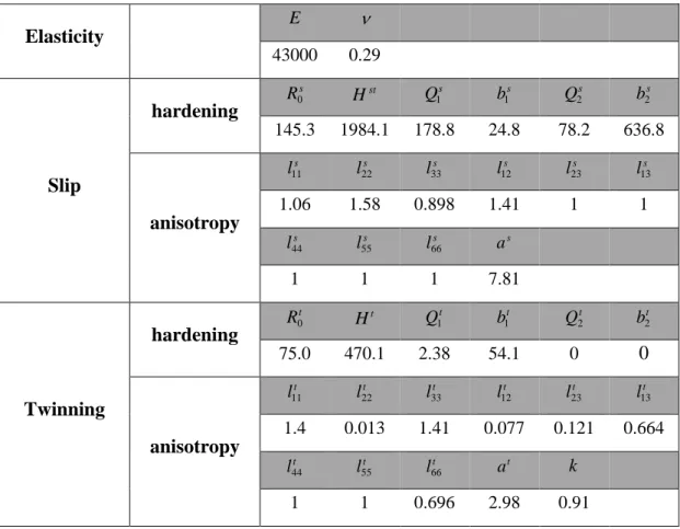
1 1 1 2 2 2 2 2 2 1 1 1 exp exp , , exp , exp . s s s s s s s s s s st s t t t t t t s t t t t t s t R R Q b b Q b b H R R Q b b H Q b b                          (65)

The material parameters corresponding to these simulations have been identified by Steglich et al. (2016) and are listed in Table 1. For these simulations, distortional hardening is neglected as all the anisotropy parameters are taken to be constant during plastic loading.

-22-

Table 1. Material parameters for the AZ31 magnesium alloy (stress-like parameters are expressed in MPa).

Elasticity

E  43000 0.29

Slip

hardening

0 s R _Hst 1 s Q _b1s 2 s Q _b2s 145.3 1984.1 178.8 24.8 78.2 636.8

anisotropy

11 s l _l22s 33 s l _l12s 23 s l _l13s 1.06 1.58 0.898 1.41 1 1 44 s l 55 s l 66 s l _as 1 1 1 7.81

Twinning

hardening

0 t R _Ht 1 t Q 1 t b 2 t Q 2 t b 75.0 470.1 2.38 54.1 0

0

anisotropy

11 t l 22 t l 33 t l 12 t l 23 t l 13 t l 1.4 0.013 1.41 0.077 0.121 0.664 44 t l 55 t l 66 t l _at _k 1 1 0.696 2.98 0.91

The initial imperfection factor f , which is equal to 0 1 0 / 0

B A

e e (Fig. 2), is set to _{5 10} 3 _{for all the}

simulations based on the M–K approach (except for the results of Fig. 6c, where the effect of 0 on

the shape and the level of the forming limit diagrams is analyzed). It should be mentioned that f 0

usually ranges from ₁₀3 _{to 2 10} 2_{. In the different figures presented in what follows, the stress}

components ( ₁₁, ₂₂, F / S₀...) are expressed in MPa.

4.2. Validation of the numerical implementation

In a preliminary stage, several numerical simulations are carried out to evaluate the accuracy of the numerical implementation of the constitutive equations with the implicit algorithm developed in Section 3.3. This evaluation is based on a number of relevant comparisons, using the parameters identified in Steglich et al. (2016), in order to assess the numerical implementation of the constitutive framework. The results of these simulations are presented in Fig. 3. Despite the complexity of the material behavior, the accuracy of the developed implicit integration scheme is clearly confirmed in Fig. 3a, where a uniaxial compression test is simulated with several strain increments 11. The

results of this figure show that the compression stress–strain curve is almost insensitive to the strain increment size. Hence, the implemented implicit algorithm provides good accuracy even when large time increments are used. Another interesting consequence of this accuracy assessment is that the use

-23-

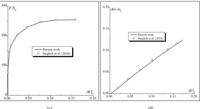
of the adaptive time step strategy, embedded in the algorithm developed in Section 3.2, allows the CPU time to be considerably reduced without loss of accuracy. To further validate our numerical implementation, comparisons between the initial yield surfaces predicted by the developed numerical tool (dotted curves) and their counterparts determined by the analytical expressions given by Eqs. (8) and (12) (solid curves) are presented in Fig. 3b. This figure confirms that the different yield criteria are correctly implemented in the developed numerical tool. The comparisons between our results and those published by Steglich et al. (2016) are given in Fig. 3c and Fig. 3d. Fig. 3c shows the evolution of the nominal stress as a function of the nominal strain, as obtained by applying a uniaxial tensile test in the longitudinal direction (which coincides here with the 1 direction). As to Fig. 3d, it depicts the evolution of the relative width reduction as a function of the nominal strain for the same test. The results of Fig. 3c and Fig. 3d reveal that the predictions obtained by the developed implicit algorithm are in excellent agreement with those reported in Steglich et al. (2016).

0.00 0.03 0.06 0.09 0.12 0.15 0 100 200 300 400 500 _ _ _ _ _ _ -150 0 150 300 450 -150 0 150 300 450 CPB06 CPB06 BLB91 BLB91 _ _ (a) (b)

-24-

0.00 0.05 0.10 0.15 0.20 0 100 200 300 Present work Steglich et al. (2016) F/S₀ l/l_ 0.00 0.05 0.10 0.15 0.20 0.00 0.05 0.10 0.15 0.20 Present work Steglich et al. (2016)  /₀ l/l_ (c) (d)

Fig. 3. Validation of the integration algorithm of the constitutive equations: (a) Accuracy of the numerical integration; (b) Validation of the implementation of the yield surfaces; (c) Comparison with results reported in

Steglich et al. (2016): tension and compression stress–strain curves; (d) Comparison with results reported in

Steglich et al. (2016): Lateral strain versus axial strain in tension.

4.3. Prediction of forming limits

The parameters given in Table 1 (Section 4.1) are used in this section to predict the mechanical behavior and the onset of necking in thin sheets. The evolutions of the accumulated slip s _and

twinning t_{, as functions of the strain component}

11

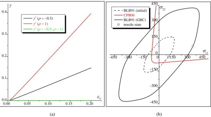
 , are displayed in Fig. 4a for two particular strain paths: the uniaxial tension strain path (  ) and the equibiaxial tension strain path (  ). This figure clearly shows that the twinning mode is not activated for both strain paths (accordingly, the corresponding accumulated twinning remains equal to 0 all along loading), and that plasticity is only due to the activation of the slip mode. To further analyze this point, we plot in Fig. 4b the initial yield surfaces and the yield surfaces corresponding to bifurcation (predicted by the GBC) for the uniaxial tensile strain path. The initial tensile state and the tensile state at bifurcation are represented by symbol ‘’. Starting from a stress-free state (1122  ) and following a uniaxial tension strain path, the

inner yield surface determines the first active plastic deformation mode. In this case, the BLB91 yield surface is firstly reached. With increasing the equivalent slip strain s_{, the material hardens and the}

BLB91 yield surface expands. On the other hand, the twinning yield surface remains unchanged, as the hardening parameter 2

t

Q ,

which

reflects the effect of the slip deformation mode on the evolution of the twinning yield function, is set to 0. Despite the increase of _{R all along the plastic deformation,} s