An experimental study of trading volume and divergence of expectations in relation to earnings announcement

Texte intégral

(1)2007s-24. An Experimental Study of Trading Volume and Divergence of Expectations in Relation to Earnings Announcement Thanh Huong Dinh, Jean-François Gajewski. Série Scientifique Scientific Series. Montréal Novembre 2007. © 2007 Thanh Huong Dinh, Jean-François Gajewski. Tous droits réservés. All rights reserved. Reproduction partielle permise avec citation du document source, incluant la notice ©. Short sections may be quoted without explicit permission, if full credit, including © notice, is given to the source..

(2) CIRANO Le CIRANO est un organisme sans but lucratif constitué en vertu de la Loi des compagnies du Québec. Le financement de son infrastructure et de ses activités de recherche provient des cotisations de ses organisations-membres, d’une subvention d’infrastructure du Ministère du Développement économique et régional et de la Recherche, de même que des subventions et mandats obtenus par ses équipes de recherche. CIRANO is a private non-profit organization incorporated under the Québec Companies Act. Its infrastructure and research activities are funded through fees paid by member organizations, an infrastructure grant from the Ministère du Développement économique et régional et de la Recherche, and grants and research mandates obtained by its research teams. Les partenaires du CIRANO Partenaire majeur Ministère du Développement économique, de l’Innovation et de l’Exportation Partenaires corporatifs Alcan inc. Banque de développement du Canada Banque du Canada Banque Laurentienne du Canada Banque Nationale du Canada Banque Royale du Canada Banque Scotia Bell Canada BMO Groupe financier Bourse de Montréal Caisse de dépôt et placement du Québec DMR Conseil Fédération des caisses Desjardins du Québec Gaz de France Gaz Métro Hydro-Québec Industrie Canada Investissements PSP Ministère des Finances du Québec Raymond Chabot Grant Thornton State Street Global Advisors Transat A.T. Ville de Montréal Partenaires universitaires École Polytechnique de Montréal HEC Montréal McGill University Université Concordia Université de Montréal Université de Sherbrooke Université du Québec Université du Québec à Montréal Université Laval Le CIRANO collabore avec de nombreux centres et chaires de recherche universitaires dont on peut consulter la liste sur son site web. Les cahiers de la série scientifique (CS) visent à rendre accessibles des résultats de recherche effectuée au CIRANO afin de susciter échanges et commentaires. Ces cahiers sont écrits dans le style des publications scientifiques. Les idées et les opinions émises sont sous l’unique responsabilité des auteurs et ne représentent pas nécessairement les positions du CIRANO ou de ses partenaires. This paper presents research carried out at CIRANO and aims at encouraging discussion and comment. The observations and viewpoints expressed are the sole responsibility of the authors. They do not necessarily represent positions of CIRANO or its partners.. ISSN 1198-8177. Partenaire financier.

(3) An experimental study of trading volume and divergence * of expectations in relation to earnings announcement Thanh Huong Dinh†, Jean-François Gajewski‡ Résumé / Abstract L’objectif de cette étude est d’observer, d’un point de vue expérimental, la réaction des investisseurs lors de la diffusion des bénéfices annuels d’une entreprise en termes de volume de transactions. Le revenu net annuel est perçu par les actionnaires comme l’indice le plus important, étant responsable de la détermination des gains individuels à l’assemblée des actionnaires. Au cours de l’expérience, cet indice est annoncé après huit rondes d’échanges. Une fraction du revenu annuel est annoncé à tous les participants une période sur deux. Ainsi, les participants révisent périodiquement leurs attentes face aux résultats annuels. L’expérience démontre que la divergence des attentes ne diminue pas lorsque les investisseurs possèdent plus d’information sur les résultats finaux. C’est ce qui explique principalement les transactions obtenues dans notre marché d’actifs expérimental. Cependant, une divergence trop importante empêche les investisseurs d’effectuer des transactions. Comme prévu, les changements de prix en valeur absolue influencent le volume de transactions. Cette conséquence est toutefois moins importante que l’impact de l’hétérogénéité des attentes. Mots clés : volume de transactions, hétérogénéité des attentes, annonce des bénéfices, marchés d’actifs expérimentaux The objective is to study from an experimental point of view investors’ reactions to the announcement of annual earnings in terms of trading volume. Annual net income is seen by shareholders as the most important figure, since it is, for individual accounts, the basis for determining profit by the shareholders’ general meeting. In the experiment, this is announced at the end of eight rounds of exchange. Every two periods, a fraction of the annual income is revealed to all the participants. Thus they periodically revise their expectations as to the annual results. The experiment shows that the divergence of expectations does not decrease when investors have more information about the final results. This is the main explanation for transactions in our experimental asset markets. However, too large a divergence prevents investors from trading. As expected, price changes in absolute value influence trading volume. But this effect is smaller than the impact of heterogeneity of expectations. Keywords: trading volume, heterogeneity of expectations, earnings announcement and experimental asset markets Codes JEL : C91 – D84 *. The experiments were carried out at CIRANO (Center for Interuniversity Research and Analysis on Organizations). We are indebted to Claude Montmarquette for his valuable help and to Julie Héroux for technical assistance in conducting this research. Financial support for the research was provided by IRG and CDC Institute for Economic Research (Caisse des Dépôts et Consignations). We particularly thank Isabelle Laudier. Finally, we have benefited from helpful comments on a preliminary version at the ISINI conference in Lille (2003), at the Northern Finance Association meeting (2004). We also thank Carole Gresse. † IRG (Institut de Recherche en Gestion – Université Paris 12 Val-de-Marne – 61 avenue du Général de Gaulle - 94010 Créteil cedex – France (Tel. : + 33 1 41 78 47 52 – Fax : + 33 1 41 78 47 34). Email: tonamiskh@yahoo.fr. ‡ IRG (Institut de Recherche en Gestion – Université Paris 12 Val-de-Marne – 61 avenue du Général de Gaulle - 94010 Créteil cedex – France (Tel. : + 33 1 41 78 47 52 – Fax : + 33 1 41 78 47 34). Email : gajewski@univ-paris12.fr ..

(4) 1. Introduction According to the efficient market hypothesis, stock prices instantly incorporate all information, and hence reflect the fundamental stock value. Beyond efficient market theory, the theorem of no trade predicts that if prices immediately adjust to a change of fundamental value when new information becomes available, no trade should occur. This theorem refers to the risk-neutral rational expectations model without asymmetric information. Under these conditions, trades occur only when investors anticipate a change in asset value or have no common knowledge or have biased expectations. In regard to the first condition, theoretical and empirical studies show that price changes cause trades. From a theoretical point of view, Kim and Verrecchia (1991) demonstrate that trading volume following earnings announcements is proportional to absolute price changes. According to Karpoff’s survey (1987), an increase of absolute prices should be associated with a rise in trades. According to the second condition, the lack of common knowledge among traders, due to asymmetric information or divergent beliefs, could explain trades following earnings announcements (Kandel and Pearson, 1995; Bamber et al., 1999). The divergence of interpretations arises either from the difference in sets of information possessed by investors at the time of publication or from the heterogeneity of beliefs on the basis of the same set of information. The first situation occurs when there is asymmetric information among traders. In this case, trading volume increases as a function of absolute price changes and the accuracy of investors’ private signals. In a heterogeneous structure of information, it may be possible to infer information from trades not revealed by prices. A large change of trading volume could signal the presence of informed traders on financial markets. Other papers (Kandel and Pearson, 1995) make the assumption of a homogeneous structure of information. All investors receive the same information (for example, the annual results). Thus, trading volume is explained by the dispersion of initial beliefs and by idiosyncratic interpretations of information. Ziebart’s (1990) paper characterizes this second component as the mean revision of expectations due to the announcement.. 2.

(5) Bamber et al. (1997) characterize opinion dispersion, which they term investors’ disagreement, by the three following factors: dispersion of initial beliefs (the variance of expectations preceding the announcement), the change in this dispersion (the difference between the dispersion before and after the announcement) and the jumbling of beliefs (the change in one investor’s beliefs relative to those of others). However, empirical studies are unable to measure directly the heterogeneity of investors’ beliefs. These are estimated by the dispersion of financial analysts’ forecasts at the time of the announcement. This proxy is open to question, since financial analysts represent only a small proportion of economic agents (Atiase and Bamber, 1994). Moreover, they have positions different from those of other agents. They are often more informed and more qualified than individual investors. Finally, their behavior strictly depends on their interests and utility functions, which is liable to induce specific biases, such as overoptimism. In this context, the experimental method may be of particular interest for this kind of research. Effects can be observed directly in a controlled environment and variables influencing trading volume can be isolated from other effects, advantages which do not arise with traditional empirical studies. The objective is thus to study the evolution of trading volume in relation to earnings announcement using the experimental method. There are three main contributions. First, traders’ heterogeneous expectations are considered independently, instead of being derived from financial analysts’ forecasts. Second, the experimental methodology isolates the heterogeneity of expectations from asymmetric information, since all the investors possess the same information. Net income is made known after the announcement of four quarterly results every two periods. The continuous flow of public information makes it possible to study the path of trades in relation to earnings announcement. Third, this structure of homogeneous information allows us to analyze further the links between trading volume, stock price variation and the heterogeneity of expectations. This relation is verified more deeply on the basis of different degrees of divergence among analysts’ forecasts. Two structures of information are constructed with different standard deviations. The second structure, with a higher standard deviation, should logically lead. 3.

(6) to a greater divergence among investors’ expectations. Instead of an increasing linear function, we observe a concave relation between trading volume and the divergence of expectations. Despite the common structure of information, the experiment shows that trades occur among participants. These trades are explained by stock price changes and the heterogeneity of expectations. The second element is the main explanatory factor for trades when divergence is not too high. Above a given threshold, divergence does not lead to any further trades. Conversely, the average change in investors’ anticipations does not influence trades. The present study also proposes that price variations positively influence trades, thus reinforcing previous conclusions that absolute price changes should entail portfolio reallocation. In addition, previous price errors also motivate trades. Moreover, it appears that divergent expectations may emerge even in a world of homogeneous information, a result similar to Gillette et al. (1999). According to these results, some investors do not seem to believe in a rational reaction on the part of other agents, and submit orders. As a consequence, market uncertainty depends not only on the process of how to determine the fundamental stock value but also on agents’ motivations. These ensure the liquidity of our experimental asset markets. For example, an optimistic trader willing to buy may not find a counterpart seller if no other trader wants to sell in the same period.. 2. Research hypotheses Obviously, interim figures are in fact perceived as an imprecise indicator of the annual results. The picture becomes increasingly detailed as the year end approaches. According to this logic, as the number of periods increase and the publication of the final results approaches, earnings expectations should become increasingly homogeneous and converge towards the value of the earnings. Hypothesis 1: Participants’ estimations of the final results converge towards the annual results as the number of periods increases. This convergence is all the faster as interim results are announced.. 4.

(7) The heterogeneity of investors’ earnings expectations positively affects trading volume, when this is not too large. Beyond a given threshold, the probability that two opposite orders can be matched is reduced. When the expectations differ too much from one investor to another, the placing orders should be widely different. The greater this divergence becomes, the more investors would take into account other agents’ behavior, thereby making the orders converge in the same direction and reducing the amount of trades. This suggests that there exists a threshold of divergence below which heterogeneity positively affects trading volume. Above it, the impact of divergence on trading volume becomes negative. Hypothesis 2: the relation between trading volume and divergence of investors’ expectations is concave.. In the present study, several degrees of dispersion are considered as two different structures of information. The first is constructed in order to entail less uncertainty than the other. Participants’ earnings expectations should logically be less heterogeneous in the first structure than in the second. An increasing and linear relationship between dispersion and trading volume should be observed in the first structure of information. Conversely, this type of relationship should be not valid in the case of the second structure. Hypothesis 2.1: in the case of the first structure of information (where expectations are not too divergent), trading volume is an increasing function of the dispersion of investors’ earnings expectations.. Hypothesis 2.2: In the case of the second structure of information (where expectations are highly divergent), the increasing relationship between trading volume and dispersion is no longer valid.. Copeland’s model (1976), extended by Epps and Epps (1976) and Jennings et al. (1981), proves theoretically that volume is positively related to the magnitude of the price change. Under the assumption of sequential arrival of information, the information leads 5.

(8) to shifts in investors’ demands, resulting in trading. This is largely confirmed by empirical studies (Karpoff, 1987 for a survey). Hypothesis 3: The magnitude of stock price variation has a positive effect on trading volume.. In addition, stock price deviations from the efficient price can also affect trading volume, since they determine trading gains that investors may have made by the end of the experiment. As a consequence, the magnitude of price errors should lead to more incentive to trade. Hypothesis 4: The size of previous price errors positively influences trading volume In the above hypothesis, previous price errors are used instead of contemporaneous ones, because contemporaneous errors are calculated only at the end of the period.. 3. Methodology This section focuses on our experimental methodology. We first describe the experimental markets in which the above research hypotheses will be examined. We then turn our attention to the determination of test parameters. 3.1. Description of experimental markets Participants and incentive Overall, the number of participants amounts to 91, divided into 11 markets. Each market has 7 to 10 unqualified students2. Using large markets makes it easier to characterize the divergence of individual reactions. The participants have no special knowledge of. 2. The present experiment only requires participants to have reasonable knowledge of the field. No specialist knowledge is needed, since various experimental studies have shown that a high skills level is not necessary to make the experiments successful.. 6.

(9) finance. They are invited to attend an initial training session where they receive detailed written instructions3. All participants are given an initial endowment of 200 Units of Experimental Cash (UEC) and 20 shares of the same stock. They react to information they receive (earnings announcement, orders, prices and trades). Their objective is to maximize their final wealth. Each participant’s total experimental gain comes from their exchange gains and earnings estimates. If positive, this is converted into cash ($CAD) and added to 10 $ of initial endowment to construct their real gain. Otherwise, the gain is considered to be zero and the participant receives only 10 $CAD. The rate of conversion is determined so that on average the participants receive 20 $CAD. The aggregate of gains is calculated as follows: 10 $CAD + Max ⎧⎨0 ; ⎛⎜ Forecast Gains + Exchange Gains ⎞⎟ ⎫⎬ ($CAD ) ⎝ ⎠⎭ ⎩. (1). Total gain. Where, Forecast gains = ∑ Forecast gain per period Forecast gain per period = Max(0 ;5 − abs( forecast error per period )) Final results announced at the end of the exp eriment Forecast error per period =. (2). − Forecast at the beginning of every period. And, Exchange gains = ∑ Capital gains + Number of shares × stock value at the end of the exp eriment − 200. (3). This premium encourages participants to improve their forecast of annual earnings. It reaches a maximum as the individual forecast at the beginning of every period approaches the final annual results.. 3. See detailed instructions in Annex.. 7.

(10) The trading price and the fundamental stock value are measured in experimental currency. In the experiment, all the shares held by participants are bought back at the end of the session at a price equal to the fundamental stock value. This rule prompts the participants to speculate about stock prices.. The structure of information Conversely to the majority of previous studies, our experiment is built on a structure of information shared by all the investors4 and made up of a flow of information leading to the final results. This model gives a good fit to reality, since there are always other sources of information before the final earnings announcement. These may be preliminary announcements of results or estimates of results, and interim publications. Hence the results are announced after four components have been revealed. Every two periods, one component is randomly chosen. Consequently, investors have increasing information as the experiment proceeds. As the uncertainty of results becomes less, investors’ earnings estimates should be increasingly accurate and homogeneous. If the linear relation is valid, trading volume should decrease as the experiment comes to an end. Two series of information about four components are provided. They have the same mean but different standard deviations in order to generate different degrees of dispersion of estimates. This may help to show the predicted concave relation between trading volume and heterogeneity of expectations, which may emerge from a high level of dispersion of expectations. Every series of four components follows Gillette et al. (1999) in terms of determination of the value of the elements. Certain differences between Gillette’s work and the present paper are related to the definition of uncertainty and the flow of information. Firstly, for Gillette et al. (1999), uncertainty about the fundamental value is explained only by the random determination of its components. For us, on the other hand, uncertainty does not lie only in the determination of the annual results but also in the relation linking the results to the fundamental stock value. For purposes of simplification, we assume that the 4. There is no asymmetric information among investors during the experiment.. 8.

(11) intrinsic value is equal to the dividend5. The latter is equal to the final results if they are positive, and zero otherwise. The second difference concerns the number of components and the set of values of each component. In Gillette et al. (1999), the final value is the sum of five positive elements, whereas the final value here is the sum of four elements. This structure of information is closer to the real-life situation, where quarterly results are announced before annual earnings. Moreover, the series may contain negative values. There are two advantages in introducing negative values: it allows firms to incur losses as well as profits; and it can help measure risk preferences. The two series of information are described as follows. For the first series, the final results are made of four elements whose value is 0, 2, 4 or 6, with probabilities ¼, ¼, ¼ and ¼. These four elements are chosen at random and announced at the end of periods 2,. 4, 6 and 8. Since they are the sum of these four elements, the final results belong to the interval [0; 24]. The dividend is distributed at the end of the experiment. For purposes of simplification, the rate of distribution is always equal to 100%. It is stable and preannounced at the beginning of the experiment. The dividend is thus equal to the fundamental value. At the beginning of every exchange round, the participants are asked to estimate the value of the results. The structure of information allows a regular estimate of the results between periods 1 and 2, 3 and 4, 5 and 6, 7 and 8. These intervals are called estimation periods. At the end of each estimation period, one element of the series of information is randomly chosen. The mean value of each component is equal to: 0× 1 + 2× 1 + 4× 1 +6 × 1 = 3 4 4 4 4. Before the first period, the expected mean value of the results is 12 and the expected fundamental value is thus 12. After the random draw of one component of the results, the objective anticipated results become the sum of this value and the estimates of the remaining elements. Draws are carried out by computer.. 5. This hypothesis does not imply that investors have the same estimation of the firm’s cost of capital or the dividend growth rate.. 9.

(12) For the second series of information, the determination of the annual results is similar to the first. However, the fundamental value is determined differently, because of one negative value in the set of possible values. In fact, the four elements of the series may take the values –4, 0, 6 or 10 with probabilities ¼, ¼, ¼ and ¼. The anticipated mean value is thus: − 4 × 1 + 0 × 1 + 6 × 1 + 10 × 1 = 3 4 4 4 4 The annual results may vary from -16 to 40 with a mean value of 12. The rate of dividend distribution is 100% if the results are positive, and zero if not. In this case, the fundamental value is equal to the dividend if it is positive and zero otherwise.. The trading mechanism We here use the structure of double-auction markets. This mechanism, which is used in the majority of stock markets, seems to be the most efficient in terms of information (Theissen (2000)) as well as in terms of allocation (Gode and Sunder (1993)). The anomalies revealed in this type of experimental market correspond closely to those found in reality, since they do not heavily depend on market microstructure. They arise mainly from the nature of the information and from the characteristics of participants such as motivations, preferences, rationality and cognitive ability. The experiment is fully computerized. First of all, stocks and cash at the participants’ disposal are registered in a virtual account. In each round, participants submit buy or sell limit orders. These orders (characterized by quantity, price and time of entry) appear continuously on all computer screens. They are recorded in a central computer that allows the execution price to be determined immediately. Trade between any two investors occurs as soon as there are opposite compatible orders. For a buy (sell) order to be executed, an investor may submit a sell (buy) order with a price limit lower than p (higher than p). Otherwise, all orders which are the same in terms of price, quantity and time of submission are implemented on a proportional basis. Short-selling is prohibited. During any one period, non-implemented orders may be modified or eliminated. They are not retained for following rounds.. 10.

(13) The evolution of the experiment Eleven markets, each with 7 to 10 students, are considered. Every market contains eight 6-minute rounds, five of which are for trades. The results are made known at the eighth round, after the announcement of four components. At the beginning of the first round, the participants are invited to estimate the annual results. This estimation stage ends when everyone has made his or her estimate. Thus participants submit orders and trade. At the end of the second round, one component of the results is randomly chosen and made known. The objective expected results are calculated as follows:. First element + 3 × 4. (4). The objective anticipated fundamental value is therefore equal to the annual results if they are positive, and zero otherwise. Subsequent rounds follow the same procedure. When one component is made known, the objective expected annual results are equal to the sum of the realized components plus the objective estimates of the remaining components. The fundamental value is always determined in the same way: it is equal to the results if they are positive, and zero otherwise. The market is completely transparent. Orders and trades are continuously shown on the screens. At the end of the eighth round, the last component is chosen randomly and the final earnings are announced. This allows the fundamental stock value to be calculated and thus the errors in investors’ expectations. 3.2. The determination of test parameters. Abnormal trading volume In this kind of study, abnormal trading volume is traditionally measured by the difference between the amount of trades during the period under consideration and the number estimated over the normal period on the basis of a standard model such as the market model. In our study, the normal period is set up in a standard way (if this is possible within the framework of the experimental study), in the sense that there is no information released and no liquidity needs. Under these conditions, the market is characterized by. 11.

(14) the absence of trading activities. In other words, abnormal trading volume is equal to zero. Therefore asset exchanges occurring in the period marked by an announcement date can be considered as the abnormal trading volume, which is thus defined as follows:. AV =. Number of traded stocks total stocks. (5). In addition to this measure, which seems to be the pure indicator of trading volume, we also consider a second proxy. Here the trading volume is equal to the ratio of the total value traded to the market’s anticipated value. The value of each transaction is equal to the quantity of assets traded times the corresponding price. The market anticipated value is simply expressed by the total number of stocks in the market times the anticipated value of associated stocks. The final measure of trading volume is derived from the second measure by modifying the denominator element. That is, we use the final value instead of the objectively estimated market value. This equals the fundamental value of stock multiplied by the total number of stocks. As this is different from the intrinsic value, which is calculated only once and at the end of the experience, rational anticipations vary in every period. Though all three of the above-mentioned measures can be used, the principal analysis and interpretations in this study are all based on the first measure, the results of which are the most relevant. In reality, the stock price can be erroneous. Its presence in the empirical tests may bias our results. It is worth noting that the only reason for using the two other measures is to compare our results with those of previous studies.. Measure of the heterogeneity of expectations The divergence of expectations is the standard deviation of individual expectations. By contrast, the homogeneity of expectations refers to the mean revision of expectations. Three measures are used in our study. The first applies to the percentage variation in expectations of a period in relation to another specified period. The next two measures are similar to the first, except that the variation in expectations is normalized differently. Respectively, they use the objective anticipated value of annual earnings and the final. 12.

(15) annual income instead of previous anticipations. The errors of expectations refer to the deviation of expectations from the final income normalized either by previous expectations or by anticipated value of earnings, or by annual earnings.. Measure of stock price variation and price errors As with the mean revision of expectations, the average variation of stock prices is determined in three ways. It is calculated as the difference between the current average price and the previous one divided respectively by the previous average price, the objective expectations of stock intrinsic value or the final fundamental value of stock. Price error is also calculated on the basis of the fundamental value. It is represented by three ratios whose numerators are the difference between stock price and intrinsic value. Their denominators, which are different from each other, correspond respectively to the average price of the previous period, the objective anticipation of true stock value and the true value.. 4. Results and interpretations. 4.1. Statistical description of earnings estimates and trading volume 4.1.1. The evolution of the earnings estimates Graphs 1.1 and 1.2 represent the percentages of expectation errors of the annual results. For information series 1, 18% of the expectations are correct, 47% are optimistic and 35% are pessimistic. Conversely, for series 2, only 7% are correct, 9% optimistic and 84% pessimistic.. 13.

(16) G r a p h 1 .1 : d is t r ib u tio n o f e s t im a te e r r o r s ( S e r ie s 1 ) 0 ,2 0. % of errors. 0 ,1 6. 0 ,1 2. 0 ,0 8. 0 ,0 4. 14. 10. 8. 6. 4. 2. 0. -2. -4. -6. -8. -1. -1. 4. 0. 0 ,0 0. E x p e c ta tio n e r r o r. G r a p h 1 .2 : d is t r ib u tio n o f e s tim a te e r r o r s ( s e r ie s 2 ) 0 ,2 0. % of errors. 0 ,1 6. 0 ,1 2. 0 ,0 8. 0 ,0 4. 10. 6. 4. -2. -4. -6. 0 -1. 4 -1. 7 -1. 9 -1. 2 -2. 4 -2. 8 -2. 2 -3. -5. 2. 0 ,0 0. E x p e c t a t io n e r r o r. Note: these graphs are made of 728 anticipations from the 11 markets. For series 1, 592 expectations are taken into account, and for series 2, 136 expectations The unexpected errors, calculated by the difference between each estimate and the annual earnings, are represented in X-plots and the percentage of expectation errors are represented in Y-plots.. 14.

(17) Graphs 1.1 and 1.2 show that, all rounds being equal, unexpected errors are numerous and highly dispersed. This high standard deviation of unexpected errors suggests that the investors do not have homogeneous anticipations, even though the experiment is based on common information, i.e., without asymmetric information. The divergence of estimates can be explained only by implicit factors that differ from one investor to another. As well as varied levels of skills and experience that directly influence the interpretation of information, further possible explanatory factors for this divergence are dissimilar risk preferences and differences in cognitive psychology. Dissimilar risk preferences may play a major role because of uncertainty during the experiment. Such uncertainty plays a part in the construction of the participants’ utility function and results in different preferences among participants. These preferences are a major determinant of expectations, since individuals have a strong tendency to invest their hopes in the real situation. The effect of investors’ risk preferences on their earnings expectations can be better defined by comparing expectations obtained from series 1 and those obtained from series 2. In series 2, with a negative component in the results, expectations are more divergent and more pessimistic than those of series 1. On average, investors are not mistaken in series 1, since the mean expectation error is -0.03, significantly different from zero. In the case of series 2, investors are rather pessimistic, with a mean expectation error of -11.15. Series 1 exhibits a standard deviation of 4.7, whereas series 2 shows a standard deviation of 10.78. In fact, the negative component introduces further uncertainty regarding the final results. In this case, risk preferences have a greater influence on investors’ behavior. In addition to the risk preference factor, the psychological and cognitive variables also explain the heterogeneity of expectations. Indeed, overconfident investors may think that they have skills superior to others and that other investors’ expectations are not correct, which leads them to form expectations at odds with the market. As a result, the divergence of expectations increases. Lack of self-confidence can also result in estimates that deviate from the fundamental value. Such investors tend to infer information from others investors’ expectations, thereby leading to mistaken expectations.. 15.

(18) G raph 2.1 : Investors' anticipation versus objective anticipation and results (series 1) 16. Value. 12. 8. 4. 0. 1. 2. 3. 4. 5. 6. 7. 8. Period Investors' anticipation. O bjective anticipation. M ean R esult. G raph 2.2 : Investors' anticipation versus objective anticipation and results (series 2) 16. Value. 12 8 4 0 1. 2. 3. 4. 5. 6. 7. 8. -4 Period Investors' anticipation. O bjective Anticipation. M ean R esult. Note: Graphs 2.1 and 2.2 incorporate all data from all markets. The exchange round is represented in X-plots, and the anticipated results, investors’ mean expectation and the final results mean in Y-plots. The objective expectation comes from a rational expectation model without asymmetric information.. 16.

(19) From graphs 2.1 and 2.2, a more detailed analysis of investors’ expectations shows that investors’ mean expectation is lower than the objective expectation. This implies that the mean expectation does not fit the rational expectations model, i.e. risk neutral and without asymmetric information. Graphs 3.1 and 3.2 show the evolution of the mean error and the standard deviation of estimates during all rounds. The evidence proves that expectation errors do not immediately converge towards zero and that the standard deviation is not significantly lower. Progressively making known the results through revealing the components does not make investors expectations more homogeneous. Hypothesis 1 is not valid. In other words, earnings expectation approaches its final value, namely that of the results, but with a time lag. There are two possible explanations for this. First, investors do not seem to have a rational and objective reaction in regard to their interpretation of the information. They fail to make increasingly precise estimations, which is contrary to their interests, since there are expectations of gains at the end of the experiment. In other words, investors’ skill in interpreting information is limited. Second, some investors are not confident in their ability to interpret information. Their behavior consists in minimizing the impact of other investors, who seem to be more sophisticated than themselves. Such minimization may be inferred from trades on the market. It entails systematic and heterogeneous errors when the “sophisticated” agents react in a divergent and erroneous way. However, the second reason seems to be less pronounced in the present study, because most participants (more than 80%) only revise their expectations at the time of an announcement. During rounds without any announcement, estimations are not modified, despite the information revealed by trades. From graphs 3.1 and 3.2, the mean and the standard deviation of expectation errors do not widely vary within the estimation periods. This phenomenon allows us to conclude that only randomly chosen elements can significantly change the formation and the revision of investors’ expectations.. 17.

(20) Graph 3.1: Evolution of unexpected errors during the experiment (series 1) 5. Error. 4 3 2 1 0 1. 2. 3. 4. 5. 6. 7. 8. Period Absolute mean expectation error. Divergence of anticipations. Graph 3.2: Evolution of unexpected errors during the experiment (series 2) 16. Error. 12. 8. 4. 0 1. 2. 3. 4 Period 5. Absolute mean expectation error. 6. 7. 8. Divergence of anticipations. Note: Graphs 3.1 and 3.2 incorporate all data from all markets. The exchange round is represented in X-plots. The expectation error and the divergence of anticipations are represented in Y-plots. All the data considered in the above graphs are calculated on average on the basis of each round.. 18.

(21) 4.1.2. The evolution of trading volume The participants trade from 1% to 53% of all shares available with a mean of 20% in series 1, and from 12% to 89% with a mean of 35% in series 2. Taking into account data from all the markets, trading volume lies between 1% and 89% with a mean of 23%. The trading volume of series 1 exhibits a slight downward trend over successive rounds. However, this is not the case for series 2.. G rap h 4: E vo lu tio n o f trad in g vo lu m e (all d ata). Trading volume. 0 ,3 0. 0 ,2 0. 0 ,1 0. 0 ,0 0 1. 2. 3. 4. Perio d. 5. 6. 7. 8. 19.

(22) G rap h 4.1: E vo lu tio n o f trad in g vo lu m e (series 1). Trading volume. 0,30. 0,20. 0,10. 0,00 1. 2. 3. 4. 5. 6. 7. 8. Perio d. G ra p h 4 .2 : E vo lu tio n o f tra d in g vo lu m e (s e rie s 2 ) 0,60. Trading volume. 0,50 0,40 0,30 0,20 0,10 0,00 1. 2. 3. 4. Perio d. 5. 6. 7. 8. Note: All three graphs show the evolution of trading volume over experiments 1 and 2. The exchange round is represented in X-plots. Trading volume expressed as the ratio “number of traded stocks/total number of stocks” is represented in Y-plots.. Despite the correlation between the objective expectations of the results across the exchange rounds, trades are not correlated between periods (even if we consider the periods without any announcement). This means that trades only come from components that are not yet announced. Further, the dispersion of investors’ reactions results rather from uncertainty in terms of future financial stock valuation.. 20.

(23) 4.2. The determinants of trading volume 4.2.1. Univariate analysis of trading volume In the present experiment, many factors may affect the fluctuations of trading volume. First, we include measures based on earnings estimates such as their heterogeneity, homogeneity and bias. Other likely determinants are variation and price errors. We thus construct a matrix of the correlation among the above variables, in which trading volume is also included. All these variables are expressed in absolute value, except for trading volume and divergence of expectations. Table1: Correlation between trading volume and its determinants Trading volume. Heterogeneity of expectations. Homogeneity of expectations. Expectation Error. Price variation. Price Error. Trading volume. 1. 0.420***. 0.125. 0.125. 0.231**. 0.326***. Heterogeneity of expectations Homogeneity of expectations Expectation Error. 0.420***. 1. 0.345***. 0.218*. 0.323***. 0.524***. 0.125. 0.345***. 1. 0.611***. 0.376***. 0.334***. 0.125. 0.218*. 0.611***. 1. 0.296***. 0.744***. Price variation. 0.231***. 0.323***. 0.376***. 0.296***. 1. 0.394***. Price Error. 0.326***. 0.524***. 0.334***. 0.744***. 0.394***. 1. Note: The table above exhibits the Pearson correlation between the variables mentioned. The tests are based on data from both series 1 and series 2, with 77 observations. *, **, *** denote significance at the 10%, 5% and 1% levels respectively.. The evidence does not confirm any significant relation between the homogeneity of expectations, anterior anticipation error and trading volume. This result remains unchanged whichever measures of homogeneity of expectations and expected error are included in the model. Among the variables shown, only divergence of expectations, price variation and price error have a significant effect on trading volume. Consequently, we carry out regression models in which the amount of trades plays the role of dependent variable and each of the significant variables indicated above is an independent variable. All the explanatory variables are expressed in absolute value except divergence of expectations.. 21.

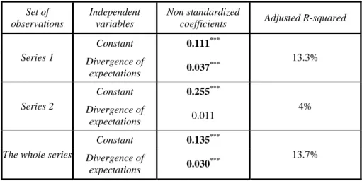
(24) 4.2.2. The impact of expectations’ heterogeneity on trading volume Since we measure the heterogeneity of expectations by dividing the standard deviation of expectations by average expectations, all the regressions presented in table 2 show how trading volume is explained by the divergence of expectations. Table 2: Impact of investors’ divergence of expectations on trading volume Set of observations Series 1. Series 2. The whole series. Independent variables. Non standardized coefficients. Constant. 0.111***. Divergence of expectations. 0.037***. Constant. 0.255***. Divergence of expectations. 0.011. Constant. 0.135***. Divergence of expectations. 0.030***. Adjusted R-squared. 13.3%. 4%. 13.7%. Note: As the standard deviation of expectations is almost constant between two announcements, data are aggregated and the regression is based on trading volume and standard deviation of all rounds. Trading volume is measured in percentage by the number of traded stocks over the number of available stocks. The divergence of expectations is equal to the standard deviation of expectations. Series 1 contains 72 usable observations and series 2 contains 16. The whole series is based on data from series 1 and series 2. *, **, *** denote significance of the test at the 10%, 5% and 1% levels respectively.. In series 1, the divergence of expectations implies a significantly positive impact on trading volume. It explains most of the variation of trades. The degree of quality of adjustment is rather high (14.5%). Hypothesis 2.1 seems to be valid. The same regression is conducted with data extracted from series 2. The results reveal an increasing but non-significant relation between the divergence of expectations and trading volume. This suggests the existence of a threshold above which the heterogeneity of expectations no longer generates trade. It seems to us that hypothesis 2.2 cannot be rejected. This type of relation, assumed to be concave, ought to be more pronounced when using higher degrees of divergence. When expectations are too dispersed, every investor becomes aware of this divergence due to the transparency of the double-auction market. In these conditions, investors become less confident and place fewer orders, thereby lowering the level of trading volume. Sometimes, however, investors do trade. 22.

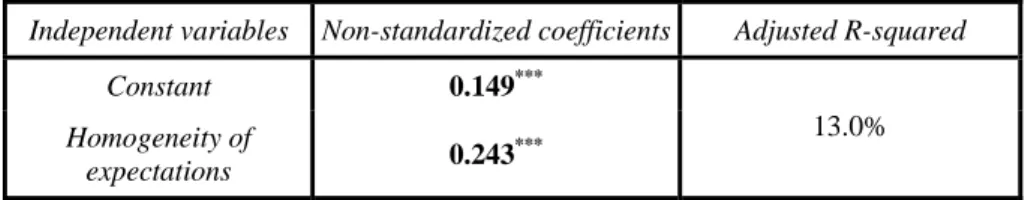
(25) without adjusting their expectations on the basis of other investors’ expectations. In this case, limit orders converge, even if the level of trading is lower. Table 2 presents the results of a regression that includes the square of the divergence of expectations. As expected, trading volume is an increasing function of heterogeneity of expectations. The significant and negative coefficient associated with the squared divergence of expectations indicates the existence of a concave relation between trading volume and heterogeneity of expectations. In other words, when this divergence becomes too large, trading volume decreases. Hypothesis 2 is entirely confirmed. Table 3: Impact of divergence of expectations and squared divergence of expectations on trading volume Independent variables. Non-standardized coefficients. Constant. Adjusted R-squared. 0.013 0.114***. Divergence of expectations Squared divergence of expectations. 20.0%. ***. -0.010. Note: data are aggregated and the regression is based on trading volume and our measure of the heterogeneity of expectations of all rounds (standard deviation of expectations). The regression is carried out with all data from series 1 and 2, i.e. 88 observations. Trading volume is measured by the number of traded stocks as a percentage of the total number of available stocks. Using other measures of trading volume leads to the same results. *, **, *** denote significance of the test at the 10%, 5% and 1% levels respectively.. Table 4 confirms the empirical results obtained with historical price data. The mean revision of expectations directly affects stock prices. If mean prices are considered as equilibrium prices, price variations should reflect the homogeneity of opinions in the market. When investors expect a rise in the results on average, stock prices should rise and, conversely, when they expect a decrease in the results, stock prices should fall. Table 4: Impact of investors’ anticipation homogeneity on stock price variation. Independent variables Constant Homogeneity of expectations. Non-standardized coefficients. Adjusted R-squared. ***. 0.149. 0.243***. 13.0%. Note: data are aggregated and the regression is based on stock price variation and mean variation of investors' expectations. The homogeneity of expectations in a period is determined by dividing the average variation of expectations by the average of previous expectations. Stock price variation is measured by the mean variation of prices. 23.

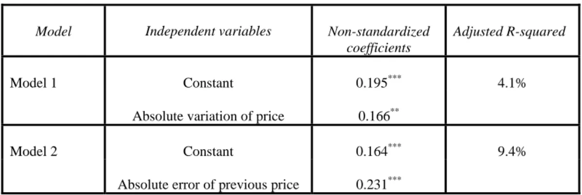
(26) divided by the mean price of the preceding period. This regression is based on all data from series 1 and 2, i.e. 88 observations. *, **, *** denote significance of the test at the 10%, 5% and 1% levels respectively.. 4.2.3. The impact of stock price variation and price errors on trading volume We now try to explain trades by stock price changes and price errors and the heterogeneity of expectations. Table 5 shows that, if considered separately, absolute price variation and previous errors have a significant impact on trading volume, which confirms hypotheses 3 and 4. Table 5: Impact of absolute price variation and previous errors on trading volume. Model. Model 1. Model 2. Independent variables. Non-standardized coefficients. Adjusted R-squared. Constant. 0.195***. 4.1%. Absolute variation of price. 0.166**. Constant. 0.164***. Absolute error of previous price. 0.231***. 9.4%. Note: All data are aggregated and the regression is based on trading volume and stock price variation. Trading volume is measured by the number of traded stocks divided by the number of available stocks. Stock price variation is measured by the variation of mean prices divided by the mean price of the preceding period. Using other measures of price variation (variation of mean prices divided by the mean expectation, variation of mean prices divided by the objective expectation, variation of mean prices divided by the annual results) leads to the same results. Excluding data from series 2 does not change the results obtained. This regression is based on 88 usable observations. *, **, *** denote significance of the test at the 10%, 5% and 1% levels respectively.. As expected we find an increasing relation between the absolute variation of absolute price and trading volume. Hypothesis 3 is valid. This result confirms the findings of previous empirical work (see Karpoff 1987). Furthermore, investors also seem to have greater incentive when they detect price errors. Hypothesis 4 does not seem to be rejected. Deviations of price from the efficient price induce investors to reallocate their portfolios in order to make large profits. In other words, operators’ motivation for trading is all the stronger when the probability of making gains is high. Moreover, the magnitude of previous price errors is likely to represent market uncertainty which, at a reasonable level, can be considered as a necessary condition in favor of trading activities. It should be noted that, in table 5, price errors are normalized by the fundamental value calculated at the end of each estimation period, i.e. every two exchange periods. In. 24.

(27) addition, this can also be calculated on the basis of the definitive fundamental value determined at the end of the session. Unlike the first measure, which leads to positive effects on trading volume, the second does not have any impact on the amount of trades. This evidence allows us to conclude that investors do not refer to the stock value determined in the long term, but to the value arising from objective expectations, calculated in the short term. This seems to be consistent with standard models in which the fundamental value is the actualized sum of future revenues (or cash-flows). The asymmetric impacts of stock price variation and errors regarding the same features of investors’ expectations puts into question the reliability of empirical studies which consider mean price variation as the average change of market opinions. This asymmetry stems from a number of elements. In fact, participants’ expectations disclose rather the individual beliefs of each independent subject, whereas stock price conveys the interaction between market operators. Therefore stock price is not only related to individual variations of each expectation, but also to the average variation of expectations. In addition, it should be noted that stock prices are not only an indicator of investors’ expectations, but also reveal the way in which these investors make up their mind when trading. Hence, prices can reflect strategies followed by market operators. The second reason seems to be relatively specific insofar as the transparency which we impose on information. In our experimental markets, individual expectations are not publicly known, whereas average prices are, a situation which corresponds to the reality of financial markets. Under these conditions, investors do not know the expectations of the others, but do know average prices. Logically, it seems that investors rely considerably on variations and errors of average prices when trading financial assets, but not on aspects of expectations. We now put the mean variation and errors of prices, as well as the divergence of investors’ expectations, in the same regression model, in which trading volume is the dependent variable. The aim of this procedure, as previously mentioned, is to test the dominance of one variable against the others. However, in such a model, we have to be careful about the interaction between independent variables, because the existence of strong linear dependences may distort the estimation results of model coefficients.. 25.

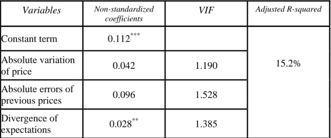
(28) We calculate the VIF statistic for our regression model where the dependent variable is the trading volume and the independent variables are composed of the divergence of investors’ expectations and the variation and errors of prices expressed in absolute value. Table 6 summarizes the results obtained. Table 6: Determinants of trading volume. Variables Constant term. Non-standardized coefficients. VIF. Adjusted R-squared. 15.2%. 0.112***. Absolute variation of price. 0.042. 1.190. Absolute errors of previous prices. 0.096. 1.528. 0.028**. 1.385. Divergence of expectations. Note: All data are aggregated. The regression is based on 88 usable observations. Trading volume is measured by the number of traded stocks in proportion of the number of stocks on the whole market. Stock price variation is measured by the relative variation of mean prices. Errors of price refer to the percentage deviation of the average price over the objective expectation of the fundamental value calculated at each estimation period. In the case of the second information series, the objectively expected value of the fundamental value can be equal to zero. For this reason all errors of price equal to zero are removed from the regression model. The divergence of investors’ expectations is the standard deviation of errors of price. In all, the first information series and both information series are based respectively on 63 and 77 observations for the model 1, and 63 and 73 observations for models 2 and 3. *, ** and *** indicate the signification of coefficients at the 10%, 5% and 1% levels.. Taking into account variables other than stock price variation leads to different results. The absolute price variation, as well as previous price errors, is no longer significant in the regression, a finding which contradicts hypothesis 3. However, the divergence of opinions still has a high significant positive impact on trading volume. In the experiment, prices significantly influence the amount of trades. However, the change is relatively homogeneous in the sense that the orders submitted are buys (sells) when prices are increasing (decreasing). In every case, the number of opposite orders is too low to lead to new trades. This phenomenon may be explained by the characteristics of the experimental markets, in that there are no traders entering or leaving the market. As a result there are no new buying or selling needs to meet existing orders, which is not the case in real markets. The existence of new traders may explain why some empirical. 26.

(29) studies reveal a relation between change in trading volume and variation of stock prices. Only the divergence of interpretations in relation to annual results has an impact on trading volume. An increasing relation between the trading volume of this experimental market and the heterogeneity of expectations is proposed when the divergence is not too high. On the other hand, divergence does not generate trading volume. A significant link has been detected between the absolute price variation and trading volume, but this factor is a lesser determinant of trading volume in comparison with divergence of opinions. To sum up, trading volume has a non-zero value despite a common structure of information for all investors. This implies that the no-trade theorem is violated. Moreover, the absence of no-trading volume is attributable not only to the change in fundamental stock value but also to investors’ different interpretations of publicly available information. The latter is a major determinant of trading volume.. 5. Conclusion The main thrust of this paper enables us to analyze the role of divergence of investors’ earnings interpretations in explaining the evolution of trades. First, investors’ expectations remain heterogeneous until the final announcement, despite successive prior announcements of results components. Moreover, these expectations do not seem to come from a rational expectations model in absence of asymmetric information. The heterogeneity of expectations accounts for a large proportion of trades on the market, unless it becomes too pronounced. The relation between trading volume and the divergence of opinions is concave. In other words, when the divergence of interpretations becomes too large, trading volume decreases. Conversely, the range of stock price variation and errors have lower impacts on trades, implying that transactions are not much leaded by price level. Only heterogeneous expectations widely result in matched buy/sell orders and hence trades. The results obtained confirm the importance of the trading volume in studies of market reaction, especially when abnormal returns seem insufficient to explain the anomalies arising from public information. In fact, trading volume indicates the heterogeneous 27.

(30) character of market reaction and complements its homogeneous aspect represented by price evolution. From these results, it may be wondered why individual expectations differ from the value arising from a rational expectations model. Why are trading prices different from the fundamental stock value? The answers to these questions call for the use of the experimental method.. 6. References. Atiase R.K. and L.S. Bamber, 1994, “Trading Volume Reactions to Annual Accounting Earnings Announcements”, Journal of Accounting and Economics, 17(3), 309-329. Bamber L.S., O.E. Barron and T.L.Stober, 1997, “Trading volume and Different Aspects of Disagreement Coincident with Earnings Announcements”, The Accounting Review, 72(4), 575-597. Bamber L.S., O.E. Barron and T.L. Stober, 1999, “Differential Interpretations and Trading Volume”, Journal of Financial and Quantitative Analysis, 34(3), 369-386. Copeland T.E., 1976, "A model of asset trading under the assumption of sequential information arrival", Journal of Finance, 31, 1149-1168. Epps T.W and Epps M.L., 1976, “The stochastic dependence of security price changes and transaction volumes: Implications for the mixture-of-distribution hypothesis”,. Econometrica, 44, 305-321. Gillette A.B., D.E. Stevens, S.G. Watts and A.W. Williams, 1999, “Price and volume reaction to public information releases: an experimental approach incorporating traders’ subjective beliefs”, Contemporary Accounting Research, 16(3), 347-379. Gode D.K. and S. Sunder, 1993, “Allocative efficiency of market with zero-intelligence traders: market as a partial substitute for individual rationality”, Journal of Political. Economy, 101(1), 119-126. Jennings R.H., Starks L.T., and Fellingham J.C, 1981, "An equilibrium model of asset trading with sequential information arrival", Journal of Finance, 36, 143-161.. 28.

(31) Kandel E. and N. Pearson, 1995, “Differential Interpretation of Public Signals and Trade in Speculative Markets”, Journal of Political Economy, 103(4), 831-872. Karpoff J.M., 1987, “The Relation between Price Changes and Trading Volume : A Survey”, Journal of Financial and Quantitative Analysis, 22(1), 109-126. Kim O. and R.E. Verrecchia, 1991, “Trading volume and price reactions to public announcements”, Journal of Accounting Research, 29(2), 302-321. Theissen E., 2000, “Market structure, informational efficiency and liquidity trading: an experimental comparison of auction and dealer markets“, Journal of Financial Markets, 3(4), 333-363. Ziebart D.A., 1990, “The association between consensus of beliefs and trading activity surrounding earnings announcements”, The Accounting Review, 65(2), 477-488.. 7. Annex. Instructions for the experiment Welcome to our experimental market, in which you can earn money. How much you gain depends on your decisions as well as those of other participants. All participants makes their decisions individually at their computers. It is strictly forbidden to communicate with the other participants. Doing so will result in your exclusion from the experiment and any gains you may have made.. You participate to a market in which you can trade stocks in order to win money by using the information contained in the right value. There are eight rounds of exchange with an initial endowment of 20 shares and 200 ECU (Experimental Cash Unit). You can buy and sell stocks from/to other participants with your cash. The gain arising from a sell is the difference between the selling price and the stock value. Conversely, the gain arising from a buy is the difference between the stock value and the buying price. The exchange gains arise from the sum of the gains arising from buys and sells. Therefore, they strictly depend on how much you can sell your stocks above or buy below the stock value. How to determine the right value. 29.

(32) Stock value is made up from the sum of four components with the same probability of occurrence. Every two periods of exchange, one component is chosen randomly by the computer. Once a draw has been made, the drawn number is always put back, so that the same numbers are always in the urn. Only one element is determined every two periods. Following the draw of an element, the subjective estimation of the stock value is recalculated. This is equivalent to the value of the preceding elements drawn and the value of the elements left to be estimated. At the end of the eighth period of exchange, the last element is drawn. The stock value is established. The draw of elements and the determination of the stock value are described in the following table. For the series 1 of information The draws are made in the sample of four numbers, 0, 2, 4 and 6. Element Value. Probability. 0. ¼. 2. ¼. 4. ¼. 6. ¼. The value of one element should be between 0 and 6 with a mean of: 0× 1 + 2× 1 + 4× 1 + 6× 1 =3 4 4 4 4. Stock value =. 1st element + 2 nd element + 3d element + 4th element. For the series 2 of information. The draws are made in the sample of four numbers, 0, 2, 4 and 6.. 30.

(33) Element Value. Probability. -4. ¼. 0. ¼. 6. ¼. 10. ¼. The value of each element should be between -4 and 10 with an expected mean of: − 4 × 1 + 0 × 1 + 6 × 1 + 10 × 1 = 3 4 4 4 4. The right value is the sum of four elements. Its range goes from -16 (when all the elements have a value of -4) to 40 (when all the elements have a value of 10). The stock value is directly extracted from the sum of the four elements, in the sense that it is equal to this sum if the latter are positive and 0 otherwise. Sum of all elements S=. Stock value. 1st element + 2 nd element + 3d element + 4th element ⎧S si S ≥ 0 V =⎨ ⎩0 si S < 0. How to make trades. The market has eight independent rounds of exchange. Each round involves three steps: -. First step. You all have to anticipate the stock value (the sum of 4 elements), not the value of each element.. -. Second step. From here on you can buy or sell stocks. On your computer, you will see a window indicating “buy” and “sell” offers. If you want to sell stocks, you should enter the selling price p. This price p indicates that your. 31.

(34) assets are sold only when the price is superior or equal to p. Conversely, if you want to buy stocks, you enter the buying price p. This price p indicates that your stocks are bought only when the price is less than or equal to p. In both cases, the quantity of traded stocks is automatically equal to 1. As a consequence, if you want to trade X stocks (X>1), you have to submit X offers. Your selling offer (or buying offer) is always added to the list of selling offers (or buying offers) appearing on your screen. It is implemented as soon as there is an offer which satisfies your price condition. However, you can also directly implement a sell or a buy by selecting an offer in the list and clicking OK. After it is implemented, the offer is withdrawn from the equivalent list. You can make offers at any time from this round onward. Non-implemented offers can be modified or cancelled in the same period. However, non-implemented offers from one period do not enter the list of trade offers of subsequent periods. -. Third step. The phase of announcement of the drawn element. A random element is announced at the end of periods 2, 4, 6, 8 and mentioned in box “drawn element”. In other periods without any announcement, the message “no element is drawn at this period” appears in the same box.. How to calculate your gains. At the end of the eighth period, all your remaining stocks are bought back at a price equal to the stock value. Your final position is based on three components. As well an initially fixed sum (part 1), you will receive a premium strictly linked to the accuracy of the expectations of the stock value (part 2) and the gains arising from your trades (part 3). The cash you win is equal to the sum of parts 1, 2 and 3, as follows:. Your final position = Part 1 + (Part 2 + Part 3)* conversion rate The rate of conversion is defined so that each of you earns from 10 to 30 Canadian dollars, with a mean of 25 $CA. Please read the instructions carefully and feel free to ask questions about anything you do not understand. The better you understand the game, the better you will be able to play.. 32.

(35)