Comparison Between Robust and Stochastic
Optimisation for Long-term Reservoir Management
Under Uncertainty
Thibaut Cuvelier · Pierre Archambeau · Benjamin Dewals · Quentin Louveaux
Received: date / Accepted: date
Abstract Long-term reservoir management often uses bounds on the reser-voir level, between which the operator can work. However, these bounds are not always kept up-to-date with the latest knowledge about the reservoir drainage area, and thus become obsolete. The main difficulty with bounds computation is to correctly take into account the high uncertainty about the inflows to the reservoir. In this article, we propose a methodology to derive minimum bounds while providing formal guarantees about the quality of the obtained solutions. The uncertainty is embedded using either stochastic or robust programming in a model-predictive-control framework. We compare the two paradigms to the existing solution for a case study and find that the obtained solutions vary substantially. By combining the stochastic and the robust approaches, we also assign a confidence level to the solutions obtained by stochastic programming. The proposed methodology is found to be both efficient and easy to implement. It relies on sound mathematical principles, ensuring that a global optimum is reached in all cases.
Keywords Long-term reservoir management · Rule curve · Stochastic optimisation · Robust optimisation
1 Introduction
Drinking-water production is a vital need, and tap water is a basic service that may not be interrupted. This water may come from multiple sources, such as groundwater or dams (surface water). Utility managers cannot afford lacking water to inject in their distribution system, and this is one reason that impelled them to build large dams and reservoirs. Those serve also multiple
Thibaut Cuvelier
other purposes, such as hydropower Bieri and Schleiss (2013) or flood control Camnasio and Becciu (2011).
These reservoirs must deliver the expected level of service with a very low probability of failure. A common management technique is to use predefined rules, i.e. rule curves. These indicate upper and lower bounds on the level of the reservoir at any period of time throughout the year Chang et al (2005). With them, the operator knows what actions are allowed on the reservoir to ensure correct operation: the water level is constrained by the prescribed rule curves. This means that no water can be released if the water level reaches the minimum-rule-curve value. Conversely, water must be released if the water level tends to approach the maximum-rule-curve value.
Modern operation of large and complex multi-reservoir systems tends to use real-time control Schwanenberg et al (2015) based on multistage mod-els Labadie (2004), instead of predefined rule curves. Multistage modmod-els in-clude recourse actions Birge and Louveaux (2011), enabling the decisions to be reconsidered over time. These models rely generally on stochastic dy-namic programming and are more intricate to implement compared to reservoir rule curves. Here, our objective is to focus on the derivation of rule curves, which prove effective for strategic planning of the reservoir management, while multistage models apply better for real-time control.
Rule-curve-based management is expected to take full advantage of the potential of the reservoirs. However, the rule curves must be periodically up-dated; otherwise, they become less reliable over time and may eventually fail to provide the expected service. The quality degradation of these operational rules is mostly due to external evolution—be they in the required amount of water or in climate change.
In this context, formal mathematical optimality guarantees of the rule curve are an asset for the operator: if there is any lack of water, the operator is able to prove that every possible action was taken to prevent this situ-ation Jordan et al (2012). To this end, mathematical optimissitu-ation can be used to derive the rule curves. With a well-defined and reproducible computational framework, the rule curves can also be regularly updated, and thus remain rel-evant, even under external evolutions. Most current optimisation techniques for reservoirs are based on evolutionary computations Ahmad et al (2014); Maier et al (2014): mostly genetic algorithms Chang et al (2005); Akbari-Alashti et al (2015), sometimes coupled with simulation Taghian et al (2014); Ahmadi Najl et al (2016), but particle swarms Spiliotis et al (2016); Peng et al (2017) and fuzzy logic Ahmadianfar et al (2017); Chen and Chang (2010) are also very common; newcomers like harmony search are gaining traction in the community Bashiri-Atrabi et al (2015). These ideas tend to be mixed together, for example fuzzy logic and genetic algorithms Sabzi et al (2016); Chaves and Kojiri (2007). The main idea behind those evolutionary techniques is to randomly explore a very large space of possible policies. Unlike evolution-ary algorithms, mathematical optimisation Labadie (2004); Zhang et al (2015); Sulis (2016) can provide global-optimality guarantees while having acceptable computational time requirements (under some assumptions, such as
convex-ity Nicklow and Mays (2000)), even for multireservoir systems. Our article demonstrates this effectiveness in the case of long-term rule curves for a single reservoir.
Whatever the optimisation method, it must take into account the inherent uncertainty in the input data (namely, the inflow). In mathematical optim-isation, there are two well-known paradigms to handle uncertainty: stochastic and robust optimisation.
1. The first is the most common one, and is also known as explicit stochastic optimisation Celeste and Billib (2009); Yeh (1985). It implies that the model directly uses probabilistic information (usually, by sampling the probability density function, i.e. using inflow scenarios for each river). The objective function minimises some risk measure Shapiro and Dentcheva (2014), often an expected value. However, in our case, the maximum func-tion makes more sense than the expectafunc-tion (see Secfunc-tion 3.2.2 for a full discussion).
2. Recently, another approach has been explored: robust optimisation Pan et al (2015), whose roots lie in mathematical optimisation communities Ben-Tal et al (2009). It considers the uncertain values as pertaining to a so-called uncertainty set and it optimises for the worst case within that set; a common choice is to use the confidence intervals around the average value. It can be considered as a kind of implicit stochastic optimisation (ISO) Celeste and Billib (2009), as the actual model is deterministic, albeit working with data that is adapted to the uncertainty. Our approach has no need for hedging the solutions to different sets of possible inflow scenarios, as it is usually necessary in ISO approaches, like in Zhao et al (2014), neither does it use linear regression as in Sulis (2016).
To the best of our knowledge, no study has so far included both paradigms to thoroughly compare them, nor used robust optimisation tools to associate a confidence level to solutions. These objective results can be useful for reservoir operators. Previous comparisons were mainly performed between one formal optimisation method and evolutionary computations, such as in Zhu et al (2017); Akbari-Alashti et al (2015).
In this paper, we compare these two paradigms based on a real-world case study of a Belgian dam on the river Vesdre, near Eupen. Historically, a very conservative process was used to compute the rule curves, with a single object-ive: water supply. We discuss to which extent the two considered approaches, robust and stochastic optimisation, may contribute to give more freedom to the operator for other purposes, such as hydropower.
Our article is structured as follows. After a brief description of the case study in Section 2, the optimisation models corresponding to each uncertainty paradigm are detailed in Section 3. The results of the optimisation process are discussed in Section 4. Finally, conclusions are drawn in Section 5, with further directions to improve this work.
2 Case study
In this study, we consider the Vesdre reservoir, which was created by dam-ming river Vesdre in Eastern Belgium immediately downstream of its junction with river Getzbach (Figure 1). River Vesdre is a tributary of river Ourthe, which is one of the main tributaries of river Meuse. The Vesdre reservoir is fed by the natural drainage area of the upper part of river Vesdre and of river Getzbach (6920 ha), as well as by another river (river Helle), from which a diversion tunnel was built. This diversion tunnel increases the effective drain-age area up to 10,595 ha. In normal-operation mode, the tunnel is open and only a minimum environmental flow remains in river Helle. If the reservoir level reaches its maximum level, the tunnel can be closed, so that the whole discharge of river Helle remains in its natural riverbed. The Vesdre dam is 50 m high and the maximum storage capacity of the reservoir is 25 hm³. The main purpose of the Vesdre reservoir is to provide drinking water. It can also be used to produce hydropower (2.6 MW) and to contribute to flood and low flow control.
The present management of the Vesdre reservoir is based on empirical rules, which are functions of the measured discharges and weather forecasts. These rules define, for each month of the year, a minimum reservoir level, above which the actual reservoir level must remain. The curve describing the variation over the year of this minimum reservoir level is called rule curve. The dam operator considers that managing the reservoir according to this rule curve guarantees the availability of drinking water for at least two years; nevertheless, no confidence level is associated to this claim.
The rule curve was derived in the 1980s, using a very conservative ap-proach. A “worst-case” scenario was defined based on historical data: for each month of the year, the reservoir inflow was assumed equal to the lowest value for the corresponding month over the period of observations. Based on this particular scenario of the reservoir inflow, a minimum reservoir level was de-termined for each month of the year, so that water supply can be ensured for a period of two years. In the following sections, we analyse how stochastic and robust optimisation may contribute to update this rule curve, by making use of today’s enhanced computational power and more recent data.
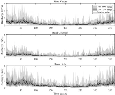
We use as main input data the characteristics of the catchment, reservoir, and dam (Tables A1 and A2 in Online Resource 1), as well as time series of observed inflow discharges to the reservoir, coming from both the natural drainage area of the reservoir (upper part of river Vesdre and river Getzbach) and from river Helle through the diversion tunnel. The corresponding time series are shown in Figure 2, as the median value over the 20 years of observa-tions (1995–2014) of daily discharge and its inter-annual variability (25%–75% and 10%–90% percentiles).
The relative number of dry and wet years in the data may influence the results of the optimisation problem. As shown in Online Resource 2, the an-nual mean inflows over the considered period are distributed relatively evenly between wet and dry years, except for river Helle: it shows some higher values
Belgium France The Netherlands Germany River Ourthe River Vesdre River Vesdre River Helle Reservoir natural drainage area Vesdre reservoir Diversion tunnel from River Helle to the Vesdre reservoir River Vesdre
River Getzbach
Figure 1: Location of the Vesdre reservoir.
for the wet years compared to the dry ones. In river Getzbach, the year 2013 was particularly wet.
3 Methodology
We developed optimisation models to compute reservoir rule curves, which define the minimum reservoir level ensuring that drinking water availability may be guaranteed even in case of a prolonged drought period. The rule curve consists in water levels at specific points during the year, called time steps. More specifically, starting from the beginning of a drought, the available drink-ing water storage must be sufficient to enable water supply durdrink-ing a predefined period of time. In the considered case study, the risk level is set such that wa-ter production must be safeguarded over a time horizon of two years, but the developed methodology may be easily adapted to other time horizons. In the following, we first define key notations (Section 3.1), then we describe the con-sidered uncertain reservoir models (Section 3.2), and finally we introduce the model-predictive-control framework used for the case study (Section 3.3).
3.1 Notations
The optimisation variables are indicated by a bold font. The value for these symbols is the result of the optimisation process, and are not fixed beforehand.
50 100 150 200 250 300 350 0 2 4 6 Discharge (m³/s) River Vesdre 10%-90% range 25%-75% range Median value 50 100 150 200 250 300 350 Time (days) 0 2 4 6 Discharge (m³/s) River Helle 50 100 150 200 250 300 350 0 2 4 6 Discharge (m³/s) River Getzbach
Figure 2: Median value of the daily discharge in River Vesdre, Getzbach and Helle over the 20 years of observations, and inter-annual variability expressed through the 25%–75% and 10%–90% percentiles.
Sets and indices. The tributary rivers are split into two groups: those that can be diverted (the set diverted) and those that cannot (the set tributaries). The index t is used to denote discrete time, i.e. the times at which a value of the rule curve is computed.
Decision variables. The real-world decision variable is the reservoir level, but we use the volume of water instead, which is in one-to-one mapping to the reservoir level. This variable is denoted by storaget (m3) at time t.
Exogenous variables. The main source of uncertainty in the case study is the inflow from each river r, written flowt,r.
Parameters. Several model parameters are fixed by the reservoir operator to fulfil the dam purposes: drinkingWatert is the drinking water demand,
environmentalFlowt is the environmental flow that must remain in the river
downstream of the reservoir.
A hydropower plant can be fed through a penstock, with penstockHydropower being the maximum discharge. The bottom outlets can also be used, with a maximum discharge of bottomOutlet. No other output from the dam is pos-sible: due to the relative position between the spillway crest and the maximum
allowable reservoir level, the spillway is not taken into account in the present model. This is consistent with the fact that we focus on the effect of droughts. Similarly, environmentalFlowr,t is the environmental flow for tributary
river r. maxDivertedr constitutes the maximum discharge capacity through
the diversion tunnel.
Bounds on the water level are also given as inputs to the model: minStorage and maxStorage are respectively the minimum and the maximum allowed volumes of water. The operator defines the minimum so that it corresponds to a reservoir level slightly above the water intakes. Similarly, the maximum level is fixed beforehand to keep a safety margin in case of floods.
3.2 Uncertain reservoir models 3.2.1 Deterministic model
The optimisation problem is mainly based on one equation, the mass balance over a time step Yeh (1985); Arunkumar and Jothiprakash (2012); Pan et al (2015):
storaget+1= storaget− outputt+ inputt, ∀t,
where the inputs correspond to the inflowing rivers, and the outputs to the various dam purposes. The inputs are composed of the tributaries and the diverted rivers: inputt= X r∈tributaries flowt,r+ X r∈diverted divertedt,r, ∀t.
For the considered case study, the output from the reservoir is the sum of the drinking water demand drinkingWatert, the minimum environmental flow in
the river environmentalFlowt, and the releases through the hydropower plant
and through the bottom outlets releaset:
outputt= drinkingWatert+ environmentalFlowt
| {z }
constant (i.e. not decided by the optimisation process)
+ releaset, ∀t.
Remark 1 Other losses could be taken into account, such as evaporation, but they are negligible in the considered area Finch and Calver (2008). Similarly, other purposes might be taken into account Castelletti et al (2008).
The constraints on minimum and maximum water levels may be expressed as: minStorage ≤ storaget≤ maxStorage, ∀t.
The contributions of the diverted rivers can be optimised as long as two con-straints are respected: a minimum environmental flow must remain in each river (and thus may not be diverted into the reservoir) and the diversion tun-nels have a maximum discharge capacity:
divertedt,r≤ flowt,r− environmentalFlowr, ∀t, ∀r ∈ diverted .
The release from the dam releasetis limited by available means of evacuating
water:
releaset≤ penstockHydropower + bottomOutlet , ∀t.
Since the overall goal is to determine an enhanced rule curve, i.e. a new lower bound for the reservoir level, the objective function minimises the total stored volume throughout the year, all periods having the same weight:
minX
t
storaget.
Thanks to this objective function, the solution is the most critical situation while still being feasible from the beginning to the end of the optimisation horizon: having a slightly lower level might endanger the required guarantees.
Remark 2 This objective is supported by the fact that, if the solver lowers the value for one time step at the expense of another, the variations for these two time steps have the same effect on the objective value. In other words, at the optimality, changing the value for any time step could force to reconsider the solution at other time steps.
All constraints detailed above and the objective function are linear. This optimisation problem is thus very tractable (large instances can be solved quickly) Vanderbei (2014). However, this model ignores the uncertainty in the inflow (i.e. flowt,r): as is, it can only consider one inflow scenario, and
optimises over that scenario, which is not representative of the actual range of possible inflows. The following sections present two approaches to incorporate the inflow uncertainty into the model while keeping it linear.
3.2.2 Stochastic model
In a first approach, we considerthe inflow as stochastic. The uncertainty is reproduced by means of a series of scenarios Shapiro and Dentcheva (2014). The rule curve is determined so that the demand for drinking water is met in all considered scenarios. Below, we first detail how the scenarios are gener-ated. Next, we present the formulation of the stochastic model enabling the computation of the rule curve.
Scenario generation. The objective of the optimisation consists in determ-ining the minimum reservoir level which guarantees drinking water availability even in the case of a M-year long drought period (in our case study, M = 2). Therefore, each scenario consists of reservoir inflows for a period of M years. Two different strategies have been tested for generating the scenarios.
– In the first one, referred to as merging, all periods of M successive years are picked in the observed time series of reservoir inflow and the corresponding values of inflow are used to define one scenario. The number of scenarios is N − M, where N is the number of years in the observation dataset (with M < N).
– In the second strategy, called mixing, a random selection of a period of one year is performed M times and the M selected periods of one year are combined to form a M-year long period. Since all possible M-tuples of one-year periods are considered, the number of scenarios is equal to NM.
As opposed to the first strategy, the second one would not preserve inter-annual correlations in the data, while both strategies keep intra-annual correlations, which are assumed stronger.
Model formulation. The computation of the rule curve is implicitly per-formed in two steps: first, each scenario is simulated independently, enabling the determination of a scenario-specific minimum reservoir level for each time step of the year; second, the rule curve is determined as the maximum, i.e. the upper envelope, of the solutions obtained for all the individual scenarios (a convex risk measure, in Shapiro and Dentcheva (2014)). The number of considered scenarios is either N − M or NM, depending on the strategy used
for generating the scenarios (respectively, merging or mixing). Let storages
tdenote the solution at time t for scenario s, and ruleStoraget
the actual value for the rule curve at time t. The rule curve must be above the minimum level for any scenario (as it is the maximum of all the solutions), which is translated by the constraint storages
t ≤ ruleStoraget. The complete
model is thus:
min P
truleStoraget
such that storages
t≤ ruleStoraget ∀t, ∀s,
storages
t+1= storagest− outputst+ input s t ∀t, ∀s, inputst=P r∈tributariesflow s t,r+ P r∈diverteddiverted s t,r ∀t, ∀s,
outputst = drinkingWatert+ environmentalFlowt+ releasest ∀t, ∀s,
minStorage ≤ storagest≤ maxStorage ∀t, ∀s,
divertedst,r≤ maxDischarger ∀t, ∀s, ∀r ∈ diverted ,
divertedst,r≤ flowst,r− environmentalFlowr ∀t, ∀s, ∀r ∈ diverted ,
releasest ≤ penstockHydropower + bottomOutlet ∀t, ∀s,
ruleStoraget≥ 0 ∀t,
storagest≥ 0, outputst≥ 0,
inputst≥ 0, releasest≥ 0 ∀t, ∀s,
divertedst,r≥ 0 ∀t, ∀s, ∀r ∈ diverted .
3.2.3 Robust model
The second uncertain model considers the inflow as belonging to an uncer-tainty set, which we chose to be the confidence interval of the inflow at the
corresponding time period based on the historical data. This choice is some-times called interval uncertainty or Soyster’s model Ben-Tal and Nemirovski (2002).
The “design” inflow to the reservoir can be computed explicitly: it corres-ponds to the minimum inflow within the confidence interval (i.e. the lower bound). As such, the robust model is very similar to the basic deterministic one which is detailed in Section 3.2.1, except in the way the inflow is chosen: it does not correspond to raw historical data, but rather the design inflow is derived from the historical data.
Various options exist for computing the confidence intervals (and thus their lower bounds). The simplest approach consists inhandling separately predefined time slices (e.g., each day of the year). In such a case,a stand-ard statistical technique may be applied to the set of values observed for each time slice (for example, January 1, January 2. . . ) over the considered time period (here, 20 years). For our case study, we used a t-Student distribution for each time step of the year. Alternate methods include fitting a dedicated statistical model (such as the one in Adam et al (2014)) or using standard time series analysis procedures (like ARMA Abrahart and See (1998)), and then modelling the residuals Spierdijk (2016).
3.3 Model predictive control (MPC)
As such, the uncertain models presented above have one important defect: they guarantee the M-year supply only for the first time step of the solution. For the following ones, the guarantee is limited by the time horizon of the model (i.e. the second time step has a guarantee for M years minus one time step). Using longer scenarios would not fix this issue properly as it would make the solution overconservative, hence suboptimal: for instance, with a M + 1-year scenario, the solution for the first time step would guarantee drinking water availability for M + 1 years (instead of two), which is more constraining than needed.
To work around this deficiency, we use M+1-year long scenarios but we per-form the optimisation on moving M-year long time horizons. In other words, the algorithm uses M + 1-year scenarios as input, but the actual optimisation (using one of the uncertain models described in Section 3.2) is performed for each time step t on a moving period of M years (i.e. from time step t to time step t + M years). This way, the result of the optimisation does match the objective of guaranteeing drinking water availability for exactly M years.
To construct the complete solution (i.e. the rule curve over the whole year), an iterative algorithm is implemented At each iteration t, it performs the following tasks:
– the optimisation problem is solved for the time period from the current time step t to time step t + M years;
– only the minimum reservoir level determined for the first time step of the current iteration (i.e. time step t) is kept to build the final solution;
Year 1 Year 2 Year 3 t1 t2 t3 t4 t5 t6
Figure 3: Behaviour of the MPC algorithm. The solution for the first time step t1 has an optimisation horizon limited to the first M years (i.e. ensures
the drinking-water guarantee for M years); the one for t2 is computed for a
M-year period starting at the second time step, i.e. the optimisation horizon of t1 shifted by one time step.
– the considered two-year time horizon is shifted by one time step (hence, starting at time step t + 1), as depicted in Figure 3.
As a consequence, the number of iterations is equal to the number of time steps in the rule curve (and as many optimisation problems are solved). Because each iteration uses exactly M years of data, the result is consistent with the objective of a M-year safety for water supply.
This technique is called receding horizon control Kwon and Han (2005). It is often used in industrial process control, including beforehand operational-rules computation (which is precisely the case here). It is part of a more generic framework, model predictive control (MPC), that has already been used with great success in water resources management, but mostly for real-time control Talsma et al (2013); Becker et al (2014).
Thanks to this algorithm, all obtained solutions are year-to-year continu-ous: there is no gap in the computed rule curve between the end of a year and the beginning of the next one. The solutions of the basic uncertain models of Section 3.2 do not have this continuity property, which is important for operators to implement the rule curve in practice.
4 Results
4.1 Outcome of the optimisation
The two described models (stochastic and robust models, both with model predictive control) have been implemented in a Julia package Bezanson et al
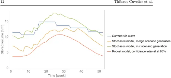
Figure 4: Comparing the two uncertainty models to the current rule curve: on the one hand, stochastic, with two scenario generation techniques; on the other one, robust.
(2017), ReservoirManagement.jl, which is freely available on GitHub1. It is
based on the JuMP mathematical modelling layer Dunning et al (2017). Both models are compared to the existing minimum rule curve in Figure 4, with weekly time steps (as the curve). Multiple rule curves have been computed for each uncertainty model:
– for the stochastic model: the two scenario generation techniques were con-sidered (merging and mixing);
– for the robust model: confidence intervals between 95% and 98.5% were tested (as detailed in Online Resource 3), whereas higher confidence levels (99% and beyond) do not allow for any solution: too little water is available in the corresponding scenarios.
Overall, the computed rule curves strongly depend on how the uncertainty is handled, i.e. stochastic or robust approach; nonetheless, the curves remain relatively close to the current rule curve; yet, at some time steps, all the proposed models are below the current rule curve. In other words, depending on the way to model the uncertainty, the current rule curve is either too conservative (none of our solutions needs a reservoir level as high as prescribed by the existing rule curve) or marginally unsafe (one model proposes to keep a slightly higher level for about one third of the year).
4.2 Associating confidence levels
By combining the stochastic and the robust approaches, we can estimate a confidence level of feasibility for the stochastic solutions. For a given solution obtained from stochastic programming, we identify a robust solution which is
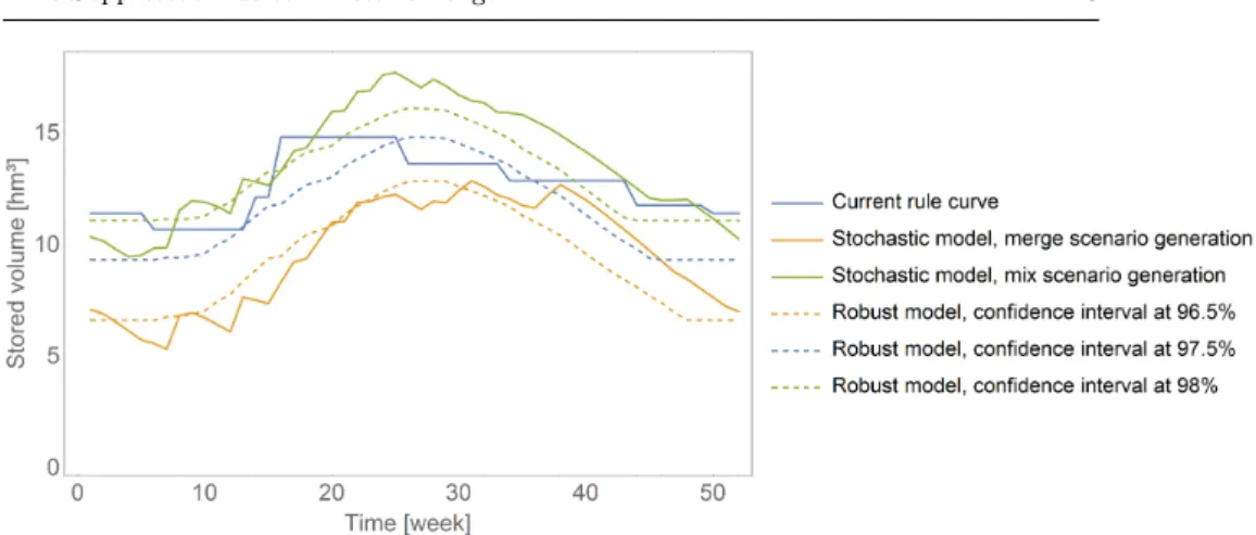
Figure 5: Closest confidence intervals corresponding to the stochastic solutions.
fairly comparable to the considered stochastic solution, and we assume that the known confidence level of the robust solution also applies to the similar stochastic solution. As shown in Figure 5, the merging scenario-generation technique leads to a confidence level of approximately 96.5%, the existing rule curve 97.5%, and the mixing scenario generation 98%.
4.3 Most important scenarios for stochastic optimisation
For the stochastic model (Section 3.2.2), there is not a single scenario that fully defines a given solution, as shown in Figure 6a: instead, a limited num-ber of scenarios have an impact on the rule curve (these scenarios may be called support vectors Cortes and Vapnik (1995)); the other scenarios have no influence on the solution.
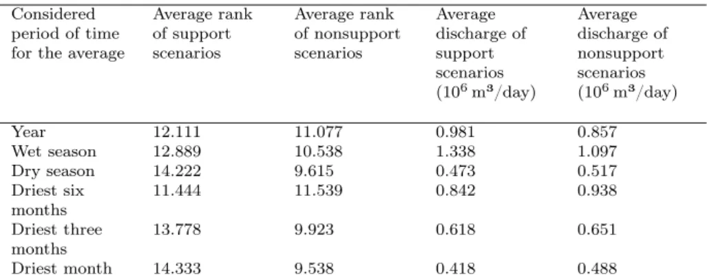
Among them, some are closer to the wettest year, others to the driest one (Figure 6a): a low average discharge throughout the scenario does not imply that it yields the most conservative solution; the distribution of the inflow over the year has a substantial influence on the result. This means that limiting the study to the driest years would not be enough to derive a sufficiently reliable minimum rule curve. In contrast, a more important factor is the driest month (as depicted in Figure 6b), as the support scenarios correspond instead to those containing some of the driest months, and these define the solution for a large period of time. Online Resource 4 presents similar results for averaging periods of three or six months, as well as for averages over the wet or the dry season. The highest correlation is observed for the driest month, but the three driest months and the dry season are similarly correlated, as indicated in Table 1. The support scenarios are not only made up of dry years, but they include also a few very wet ones. Also, these results suggest that the month is a very relevant time scale for defining the rule curve.
(a) The colour of the scenario curve corresponds to the average discharge: the bluer curves indicate a wetter year.
(b) The colours correspond to the average discharge during the driest month: the reddest curve indicates the driest month among all the scenarios.
Figure 6: Impact of the scenarios on the solution for a stochastic solver (here, merging is depicted, without MPC). The optimisation curves (i.e. the result of the optimisation and the scenarios) correspond to a 2-year scenario; each of them is plotted against the original rule curve for the first year. The colour scales are relative: dark blue indicates the wettest scenario, dark-red the driest scenario. A dashed line indicates a support scenario.
The main conclusion for the optimisation of this analysis is that the time step for the optimisation of this model should never be longer than one month, otherwise the resulting rule curve may miss some important events. It also gives an easy (but approximate) criterion to discriminate support scenarios from redundant ones, based on the driest month contained in the time series.
Table 1: Analysis of the time periods that define the optimisation results. There are 22 scenarios, of which 9 are support scenarios.
Considered period of time for the average
Average rank of support scenarios Average rank of nonsupport scenarios Average discharge of support scenarios (106m³/day) Average discharge of nonsupport scenarios (106m³/day) Year 12.111 11.077 0.981 0.857 Wet season 12.889 10.538 1.338 1.097 Dry season 14.222 9.615 0.473 0.517 Driest six months 11.444 11.539 0.842 0.938 Driest three months 13.778 9.923 0.618 0.651 Driest month 14.333 9.538 0.418 0.488 5 Conclusion
This article compares two paradigms to take uncertainty into account within mathematical optimisation techniques applied to rule-curve derivation: one is similar to many existing tools (stochastic programming), with scenario gen-eration to help deal with limited data; the other one is more synthetic and directly uses confidence levels (robust programming). Our results show that the current operating guidelines can be improved at some points. We also as-signed a confidence level to the current rule curve, and showed that moving to the mixing scenario-generation technique or to robust programming might improve water-supply safety. Moreover, the dam operator can implement any of our techniques in such a way that rule curves are regularly updated.
Besides those practical issues, the proposed methodology is easy to imple-ment with a high efficiency, while being based on sound mathematical prin-ciples. Also, the mathematical models used in this article are exploited to their utmost potential: there is no point in pursuing the research to get better solu-tions to these models, as the global optimality has been reached. Nevertheless, the models could still be improved to get more detailed results. For example, the discharge through the hydropower penstock and the bottom outlets both depend on the hydraulic head, while they are currently considered as con-stants. Another weak point is the computation of inflow confidence intervals, which is crude, and could be greatly enhanced.
Furthermore, this approach is directly applicable to any kind of water de-mand, such as controlling low flows, as long as there is no uncertainty in this demand. Otherwise, another stage of uncertainty modelling is needed, applying the same techniques as developed in this article.
The rule curves have been evaluated with feasibility-related criteria, which are the most relevant in this case for the operator. Nevertheless, other eval-uation processes could bring more information about the behaviour of each
potential policy with respect to the other dam purposes, such as hydropower like in Arunkumar and Jothiprakash (2012).
The approach can also be extended to handle flooding, by defining a max-imum rule curve for normal operations: this lets some free space to store the excess water due to flood events. This could be computed, season per season, by analysing the maximum level so that the usual constraints are not violated (as done in Section 3), with the flood event as input. This extension would require some flood detection algorithm, as presented in Klopstra and van Eck (1999).
Acknowledgements The authors gratefully acknowledge the Service Public de Wallonie (SPW) for providing data on the case study. They also thank Sébastien Erpicum for his help with the revision of the manuscript.
Conflict of interest The authors declare that they have no conflict of interest.
——————— References
Abrahart RJ, See L (1998) Neural Network vs. ARMA Modelling: constructing benchmark case studies of river flow prediction. In: Proceedings of the 3rd International Conference on GeoComputation, Bristol, URL http://www. geocomputation.org/1998/05/gc{_}05.htm
Adam N, Erpicum S, Archambeau P, Pirotton M, Dewals B (2014) Stochastic Modelling of Reservoir Sedimentation in a Semi-Arid Watershed. Water Re-sources Management 29(3):785–800, DOI 10.1007/s11269-014-0843-4, URL http://dx.doi.org/10.1007/s11269-014-0843-4
Ahmad A, El-Shafie A, Razali SFM, Mohamad ZS (2014) Reservoir Op-timization in Water Resources: a Review. Water Resources Management 28(11):3391–3405, DOI 10.1007/s11269-014-0700-5, URL http://dx.doi. org/10.1007/s11269-014-0700-5
Ahmadi Najl A, Haghighi A, Vali Samani HM (2016) Simultaneous optimiz-ation of operating rules and rule curves for multireservoir systems using a self-adaptive simulation-GA model. Journal of Water Resources Planning and Management 142(10):4016,041
Ahmadianfar I, Adib A, Taghian M (2017) Optimization of multi-reservoir op-eration with a new hedging rule: application of fuzzy set theory and NSGA-II. Applied Water Science 7(6):3075–3086
Akbari-Alashti H, Haddad OB, Mariño MA (2015) Application of fixed length gene genetic programming (FLGGP) in hydropower reservoir operation. Wa-ter resources management 29(9):3357–3370
Arunkumar R, Jothiprakash V (2012) Optimal Reservoir Operation for Hydropower Generation using Non-linear Programming Model. Journal of The Institution of Engineers (India): Series A 93(2):111–
120, DOI 10.1007/s40030-012-0013-8, URL http://dx.doi.org/10.1007/ s40030-012-0013-8
Bashiri-Atrabi H, Qaderi K, Rheinheimer DE, Sharifi E (2015) Application of Harmony Search Algorithm to Reservoir Operation Optimization. Water Resources Management 29(15):5729–5748, DOI 10.1007/s11269-015-1143-3, URL http://dx.doi.org/10.1007/s11269-015-1143-3
Becker BPJ, Schruff T, Schwanenberg D (2014) Modellierung von reaktiver Steuerung und Model Predictive Control. In: 37. Dresdner Wasserbaukolloquium 2014, URL https://izw.baw. de/publikationen/dresdner-wasserbauliche-mitteilungen/0/ 18{_}Heft{_}50{_}Modellierung{_}reaktive{_}Steuerung.pdf
Ben-Tal A, Nemirovski A (2002) Robust optimization: methodology and ap-plications. Mathematical Programming 92(3):453–480
Ben-Tal A, El Ghaoui L, Nemirovski A (2009) Robust optimization. Princeton University Press
Bezanson J, Edelman A, Karpinski S, Shah VB (2017) Julia: A Fresh Approach to Numerical Computing. SIAM Review 59(1):65–98, DOI 10.1137/141000671, URL http://julialang.org/publications/ julia-fresh-approach-BEKS.pdf
Bieri M, Schleiss AJ (2013) Analysis of flood-reduction capacity of hydro-power schemes in an Alpine catchment area by semidistributed concep-tual modelling. Journal of Flood Risk Management 6(3):169–185, DOI 10. 1111/j.1753-318X.2012.01171.x, URL http://doi.wiley.com/10.1111/j. 1753-318X.2012.01171.x
Birge JR, Louveaux F (2011) Introduction to Stochastic Programming, 2nd edn. Springer Verlag, DOI 10.1007/978-1-4614-0237-4, URL http://www. springer.com/mathematics/applications/book/978-1-4614-0236-7 Camnasio E, Becciu G (2011) Evaluation of the Feasibility of
Irriga-tion Storage in a Flood DetenIrriga-tion Pond in an Agricultural Catch-ment in Northern Italy. Water Resources ManageCatch-ment 25(5):1489– 1508, DOI 10.1007/s11269-010-9756-z, URL http://dx.doi.org/10. 1007/s11269-010-9756-z
Castelletti A, Pianosi F, Soncini-Sessa R (2008) Water reservoir control un-der economic, social and environmental constraints. Automatica 44(6):1595– 1607, DOI http://dx.doi.org/10.1016/j.automatica.2008.03.003, URL http: //www.sciencedirect.com/science/article/pii/S0005109808001271 Celeste AB, Billib M (2009) Evaluation of stochastic reservoir operation
op-timization models. Advances in Water Resources 32(9):1429–1443, DOI 10.1016/j.advwatres.2009.06.008, URL http://www.sciencedirect.com/ science/article/pii/S0309170809001006
Chang FJ, Chen L, Chang LC (2005) Optimizing the reservoir operating rule curves by genetic algorithms. Hydrological Processes 19(11):2277–2289, DOI 10.1002/hyp.5674, URL http://doi.wiley.com/10.1002/hyp.5674 Chaves P, Kojiri T (2007) Stochastic fuzzy neural network: case study of
op-timal reservoir operation. Journal of Water Resources Planning and Man-agement 133(6):509–518
Chen HW, Chang NB (2010) Using fuzzy operators to address the complexity in decision making of water resources redistribution in two neighboring river basins. Advances in water resources 33(6):652–666
Cortes C, Vapnik V (1995) Support-vector networks. Machine Learning 20(3):273–297, DOI 10.1007/BF00994018, URL http://dx.doi.org/10. 1007/BF00994018
Dunning I, Huchette J, Lubin M (2017) JuMP: A Modeling Language for Mathematical Optimization. SIAM Review 59(2):295–320, DOI 10.1137/ 15M1020575
Finch J, Calver A (2008) Methods for the quantification of evapora-tion from lakes. Tech. rep., URL http://nora.nerc.ac.uk/14359/1/ wmoevap{_}271008.pdf
Jordan FM, Boillat JL, Schleiss AJ (2012) Optimization of the flood protection effect of a hydropower multi-reservoir system. International journal of river basin management 10(1):65–72
Klopstra D, van Eck NV (1999) Methodiek voor vaststelling van de vorm van de maatgevende afvoergolf van de Maas bij Borgharen. HKV Lijn in Water in opdracht van WL|Delft Hydraulics en Rijkswaterstaat RIZA
Kwon WH, Han SH (2005) Receding Horizon Control: Model Predictive Con-trol for State Models, 1st edn. Springer-Verlag London, DOI 10.1007/ b136204, URL http://www.springer.com/us/book/9781846280245 Labadie JW (2004) Optimal Operation of Multireservoir Systems:
State-of-the-Art Review. Journal of Water Resources Planning and Management 130(2):93–111, DOI doi:10.1061/(ASCE)0733-9496(2004)130:2(93), URL http://ascelibrary.org/doi/abs/10.1061/(ASCE)0733-9496(2004) 130:2(93)
Maier HR, Kapelan Z, Kasprzyk J, Kollat J, Matott LS, Cunha MC, Dandy GC, Gibbs MS, Keedwell EC, Marchi A, Ostfeld A, Savic D, Solomatine DP, Vrugt JA, Zecchin AC, Minsker BS, Barbour EJ, Kuczera G, Pasha F, Castelletti A, Giuliani M, Reed PM (2014) Evolutionary algorithms and other metaheuristics in water resources: Current status, research chal-lenges and future directions. Environmental Modelling & Software 62:271– 299, DOI http://dx.doi.org/10.1016/j.envsoft.2014.09.013, URL http:// www.sciencedirect.com/science/article/pii/S1364815214002679 Nicklow JW, Mays LW (2000) Optimization of multiple reservoir networks for
sedimentation control. Journal of hydraulic engineering 126(4):232–242 Pan L, Housh M, Liu P, Cai X, Chen X (2015) Robust stochastic optimization
for reservoir operation. Water Resources Research 51(1):409–429
Peng Y, Peng A, Zhang X, Zhou H, Zhang L, Wang W, Zhang Z (2017) Multi-Core parallel particle swarm optimization for the operation of Inter-Basin water transfer-supply systems. Water Resources Management 31(1):27–41 Sabzi HZ, Humberson D, Abudu S, King JP (2016) Optimization of adaptive
fuzzy logic controller using novel combined evolutionary algorithms, and its application in Diez Lagos flood controlling system, Southern New Mexico. Expert Systems with Applications 43:154–164
Schwanenberg D, Becker BPJ, Xu M (2015) The open real-time control (RTC)-Tools software framework for modeling RTC in water resources sytems. Journal of Hydroinformatics 17(1):130 LP —- 148, URL http: //jh.iwaponline.com/content/17/1/130.abstract
Shapiro A, Dentcheva D (2014) Lectures on stochastic programming: modeling and theory, vol 16, 2nd edn. SIAM
Spierdijk L (2016) Confidence intervals for ARMA–GARCH value-at-risk: The case of heavy tails and skewness. Computational Statistics & Data Analysis 100:545–559
Spiliotis M, Mediero L, Garrote L (2016) Optimization of hedging rules for reservoir operation during droughts based on particle swarm optimization. Water Resources Management 30(15):5759–5778
Sulis A (2016) An optimisation model for reservoir operation. In: Proceedings of the Institution of Civil Engineers-Water Management, Thomas Telford Ltd, pp 1–9
Taghian M, Rosbjerg D, Haghighi A, Madsen H (2014) Optimization of Con-ventional Rule Curves Coupled with Hedging Rules for Reservoir Operation. Journal of Water Resources Planning and Management 140(5):693–698, DOI 10.1061/(ASCE)WR.1943-5452.0000355, URL http://ascelibrary. org/doi/abs/10.1061/(ASCE)WR.1943-5452.0000355
Talsma J, Patzke S, Becker BPJ, Goorden N, Schwanenberg D, Prinsen G (2013) Application of Model Predictive Control on Water Extractions in Scarcity Situations in the Netherlands. Revista de Ingeniería Innova 6:1–10 Vanderbei RJ (2014) Linear Programming, International Series in Operations Research & Management Science, vol 196, 4th edn. Springer US, Boston, MA, DOI 10.1007/978-1-4614-7630-6, URL http://link.springer.com/ 10.1007/978-1-4614-7630-6
Yeh WWG (1985) Reservoir Management and Operations Models: A State-of-the-Art Review. Water Resources Research 21(12):1797–1818, DOI 10.1029/ WR021i012p01797, URL http://dx.doi.org/10.1029/WR021i012p01797 Zhang Y, Jiang Z, Ji C, Sun P (2015) Contrastive analysis of three par-allel modes in multi-dimensional dynamic programming and its applica-tion in cascade reservoirs operaapplica-tion. Journal of Hydrology 529, Part:22–34, DOI http://dx.doi.org/10.1016/j.jhydrol.2015.07.017, URL http://www. sciencedirect.com/science/article/pii/S0022169415005144
Zhao T, Zhao J, Lund J, Yang D (2014) Optimal Hedging Rules for Reser-voir Flood Operation from Forecast Uncertainties. Journal of Water Re-sources Planning and Management Preview(2011), DOI 10.1061/(ASCE) WR.1943-5452.0000432
Zhu X, Zhang C, Fu G, Li Y, Ding W (2017) Bi-Level Optimization for Determining Operating Strategies for Inter-Basin Water Transfer-Supply Reservoirs. Water Resources Management pp 1–18