& Astrophysics manuscript no. Plaskett October 7, 2014
Short-term spectroscopic variability of Plaskett’s star
?
M. Palate and G. Rauw
Institut d’Astrophysique et de Géophysique, Université de Liège, Bât. B5c, Allée du 6 Août 17, 4000 Liège, Belgium
Received 10 February 2014/ Accepted 30 September 2014
ABSTRACT
Context.Plaskett’s star (HD 47129) is a very massive O-star binary in a post Roche-lobe overflow stage. CoRoT observations of this system revealed photometric variability with a number of frequencies.
Aims.The aim of this paper is to characterize the variations in spectroscopy and investigate their origin.
Methods.To sample its short-term variability, HD 47129 was intensively monitored during two spectroscopic campaigns of six nights each. The spectra were disentangled and Fourier analyses were performed to determine possible periodicities and to investigate the wavelength dependence of the phase constant and the amplitude of the periodicities.
Results. Complex line profile variations are observed. Frequencies near 1.65, 0.82, and 0.37 d−1 are detected consistently in the He i λ 4471, He ii λ 4542, and N iii λ 4510-4518 lines. These frequencies are consistent with those of the strongest signals detected in photometry. The possibilities that these variations stem from pulsations, a recently detected magnetic field or tidal interactions are discussed.
Conclusions.Whilst all three scenarios have their strengths, none of them can currently account for all the observed properties of the line profile variations.
Key words. stars: early-type – stars: oscillations – stars: individual: HD 47129 – binaries: general
1. Introduction
The massive binary nature of HD 47129 was first reported by Plaskett (1922), who inferred a total mass of 138.9 M , the
high-est ever observed at that time. He described the binary as con-sisting of two early-type stars: an Oe5 primary and a fainter secondary with weak and broad lines. For almost a century, HD 47129, also known as Plaskett’s star, has been the target of many studies, with tremendous progress in the past twenty years (e.g. Bagnuolo et al. 1992, Wiggs & Gies 1992, Linder et al. 2006, 2008, Mahy et al. 2011, Grunhut et al. 2013a). The masses of the components have been revised downwards to m1 sin3i= 45.4 for the primary and m2 sin3i= 47.3 M for
the secondary, leading to a mass ratio of about 1.05 ± 0.05 (Lin-der et al. 2008). Unfortunately, Plaskett’s star is a non-eclipsing binary, preventing a precise determination of its orbital inclina-tion. The latter was estimated from polarimetry to 71 ± 9◦(Rudy & Herman 1978). Plaskett’s star is usually considered a member of the Mon OB2 association. However, Linder et al. (2008) find a discrepancy between the luminosity and the dynamical masses of the two components of the system, which could be solved by assuming a greater distance for the star.
In many respects, HD 47129 offers a textbook example of evolutionary effects and the effects of interactions in massive bi-naries. Linder et al. (2008) used a disentangling technique, based on the method of González & Levato (2006), on high-resolution optical spectra to derive the spectral types O8 III/I and O7.5 V/III for the primary and secondary stars, respectively. The broad and shallow absorption lines of the secondary star suggest that this star rotates rapidly (v sin i ∼ 300km s−1), whereas the much
? Based on observations collected at the Observatoire de Haute Provence (OHP, France).
sharper absorption lines of the primary indicate a projected rota-tional velocity of v sin i ∼ 75km s−1 (Linder et al. 2008). Using
the CMFGEN model atmosphere code (Hillier & Miller 1998) to analyse the disentangled spectra, Linder et al. (2008) show that the atmosphere of the primary has an enhanced N and He abun-dance and a depletion of C. The secondary atmosphere is possi-bly depleted in N. These results indicate that the binary system is in a post-Roche lobe-overflow evolutionary stage where matter and angular momentum have been transferred from the primary to the secondary.
Because of its high rotation speed, the wind of the secondary star could be rotationally flattened. Such a situation would af-fect the properties of the wind interaction zone in this binary. This was confirmed by the studies of the Hα emission region by Wiggs & Gies (1992) and Linder et al. (2008), as well as by the study of the X-ray emission of the system by Linder et al. (2006). An alternative explanation for the origin of the equatorial wind of the secondary could be magnetic confinement. Indeed, Grunhut et al. (2013a) have recently reported the presence of a magnetic field in Plaskett’s star. In the framework of the mag-netism in massive stars (MiMeS) survey, they detected Zeeman signatures from the rapidly rotating secondary in high-resolution Stokes V spectra. The strength of the highly organized field has to be at least 2850 ± 500 G, and variations compatible with rota-tional modulation of an oblique field were also found (Grunhut et al. 2013a).
Mahy et al. (2011) studied the CoRoT (Convection, Rotation, and planetary Transits, Baglin et al. 2006; Auvergne et al. 2009) light curve of Plaskett’s star and extracted 43 significant fre-quencies. Among these frequencies there are three major groups: 0.823 d−1and six harmonics, the orbital frequency 0.069 d−1and two harmonics, as well as two frequencies at 0.368 d−1and 0.399
A&A proofs: manuscript no. Plaskett Table 1. Summary of the time sampling of the observing campaigns.
Campaign Starting and ending dates Starting and ending n <S/N> ∆T < ∆t > ∆νnat νmax
(HJD-2450000) phases (days) (hours) (days)−1 (days)−1
2009 5174.415 - 5179.665 0.47 - 0.84 68 180 5.25 0.40 1.90 10−1 119
2010 5539.454 - 5543.657 0.83 - 0.12 50 146 4.20 0.55 2.38 10−1 87.7
Notes. Note that for both campaigns, there are no observations for one night due to bad weather. n is the total number of spectra,<S/N> indicates the mean signal-to-noise ratio,∆T indicates the total time between the first and last observations, ∆t provides the average time interval between two consecutive exposures of a same night. The last two columns indicate the natural width of the peaks in the periodogram∆νnat = ∆T−1and νmax= (2 < ∆t >)−1provides an indication of the highest frequency that can possibly be sampled with our time series.
d−1. The latter two could be related to the rotation period of the secondary.
The discovery of the 0.823 d−1 frequency by Mahy et al. (2011) prompted us to perform a spectroscopic monitoring of the system, to constrain the origin of this variation. In this pa-per, we report the results of this study. The paper is organized as follows. Sect. 2 describes the observations, data reduction and disentangling treatment. In Sect. 3, the line profile variations are discussed and the results of the Fourier analyses are given. Fi-nally, in Sect. 4, we discuss the strengths and weaknesses of three possible scenarios and summarize our results and conclusions.
2. Observations and data reduction 2.1. OHP spectroscopy
Spectroscopic time series of HD 47129 were obtained dur-ing two six-nights observdur-ing campaigns in December 2009 and December 2010 at the Observatoire de Haute Provence (OHP, France). We used the Aurélie spectrograph fed by the 1.52 m telescope. The spectrograph was equipped with a 1200 lines mm−1grating blazed at 5000 Å and a CCD EEV42-20
de-tector with 2048 × 1024 pixels of 13.5 µm2. Our set-up covered the wavelength domain from 4460 to 4670 Å with a resolving power of 20000. Typical exposure times were 20 – 30 minutes, depending on the weather conditions, and a total of 118 spectra were collected. To achieve the most accurate wavelength cali-bration, Th-Ar lamp exposures were taken regularly over each observing night (typically once every 90 minutes).
The data were reduced using the MIDAS software provided by ESO. The normalization was done self-consistently using a series of continuum windows. Table 1 provides a summary of our observing campaigns and the characteristics of the sampling.
2.2. Disentangling
The goal of the present paper is to study and interpret the short-term line profile variability of Plaskett’s star. Because of the Doppler shifts and line blending induced by the orbital motion in such a binary system, it is not trivial to know which star trig-gers the variations. The first step in our analysis was thus to dis-entangle the spectra of the primary and secondary components. For this purpose, we applied our code based on the González & Levato (2006) technique to the data of the two observing cam-paigns simultaneously. This method allows to derive the radial velocities as well as the individual spectra of the components. However, because of the very broad and shallow lines of the sec-ondary, its radial velocities (RVs) obtained with the disentan-gling were sometimes not well constrained. To avoid artefacts, we thus fixed the RVs of the secondary to the theoretical val-ues derived from the orbital solution of Linder et al. (2008). The
situation for the primary was better, as we recovered RVs that were in good agreement with the orbital solution of Linder et al. (2008): the dispersions of the RVs about the latter orbital so-lution were 11 and 6 km s−1for the He i λ 4471 and He ii λ 4542
lines, respectively. There were very little differences between the disentangled spectrum of the primary obtained with either the primary RVs being fixed to the orbital solution or allowing them to vary. In the subsequent analysis of the line profile variability, we thus adopted the mean spectra as reconstructed keeping the RVs of the primary fixed to the orbital solution of Linder et al. (2008). The reconstructed spectra of the individual components are displayed in Fig. 1. These individual spectra are important to correctly interpret the results of our line profile variability anal-ysis. For instance, Fig. 1 reveals that the only secondary line that has at least some parts of its profile that are not blended with primary lines at some orbital phases is He i λ 4471. The latter line displays weak emission humps that were already noted by Linder et al. (2008).
Fig. 1. Mean disentangled spectra of the primary and secondary (shifted upwards by 0.1 continuum units). Important spectral lines are identified by the labels.
3. Variability analysis 3.1. He i λ 4471
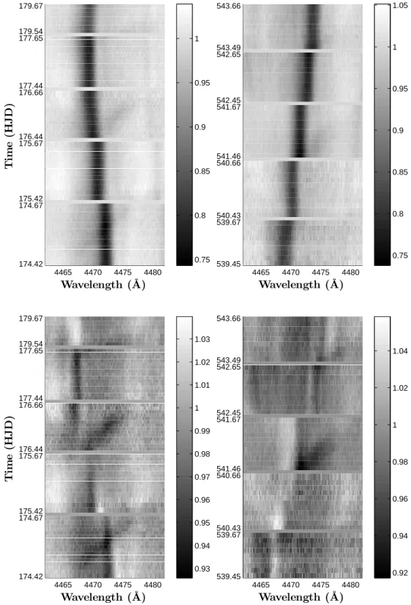
The top panels of Fig. 2 display the dynamic spectra of the observed data in the heliocentric frame of reference (hereafter called the raw dynamic spectra), whilst the bottom panels illus-trate the dynamic spectra after subtracting the mean disentan-gled primary spectrum and shifting the data into the secondary’s
4465 4470 4475 4480 174.42 174.67 175.42 175.67 176.44 176.66 177.44 177.65 179.54 179.67 Wavelength (˚A) T im e (H J D ) 0.75 0.8 0.85 0.9 0.95 1 4465 4470 4475 4480 539.45 539.67 540.43 540.66 541.46 541.67 542.45 542.65 543.49 543.66 Wavelength (˚A) 0.75 0.8 0.85 0.9 0.95 1 1.05 4465 4470 4475 4480 174.42 174.67 175.42 175.67 176.44 176.66 177.44 177.65 179.54 179.67 Wavelength (˚A) T im e (H J D ) 0.93 0.94 0.95 0.96 0.97 0.98 0.99 1 1.01 1.02 1.03 4465 4470 4475 4480 539.45 539.67 540.43 540.66 541.46 541.67 542.45 542.65 543.49 543.66 Wavelength (˚A) 0.92 0.94 0.96 0.98 1 1.02 1.04
Fig. 2. Line-profile variations in the He i λ 4471 line in the 2009 (left) and 2010 (right) campaigns. The top panels show the dynamic spectra of the observed data in the heliocentric frame of reference. The bottom panels yield the secondary dynamic spectra. The labels on the vertical axis indicate the date of the first and last observation of each night in the format HJD-2455000.
frame of reference (hereafter called the secondary dynamic spec-tra).
The raw dynamic spectra are dominated by the orbital mo-tion of the relatively sharp primary line. These figures show which parts of the core of the secondary absorption are most
affected by blends with the primary. We note that the observed position of the primary line slightly deviates from the position expected from the orbital solution. Another feature that can be seen on the first and third night of the 2009 campaign as well as on the third night of the 2010 data is a discrete depression
A&A proofs: manuscript no. Plaskett 4465 4470 4475 4480 0 0.5 1 1.5 2 Wavelength (˚A) F re q u en cy (d − 1) 0.005 0.01 0.015 0.02 0.025 0.03 0 1 2 3 4 5 0 0.1 0.2 0.3 0 1 2 3 4 5 0 0.1 0.2 0.3 0 1 2 3 4 5 0 0.2 0.4 0.6 0.8 1 4465 4470 4475 4480 0 0.5 1 1.5 2 Wavelength (˚A) F re q u en cy (d − 1) 2 4 6 8 10 12 14 16 18 x 10−3 0 1 2 3 4 5 0 0.1 0.2 0.3 0 1 2 3 4 5 0 0.1 0.2 0.3 0 1 2 3 4 5 0 0.2 0.4 0.6 0.8 1
Fig. 3. Fourier power spectra of the 2009 (left) and 2010 (right) time se-ries of the secondary’s He i λ 4471 line. The top panels of each row show the full 2D periodograms (between 0 and 2 d−1), whilst the second and third pan-els illustrate the mean periodogram over the emission humps, respectively before and after prewhitening (see text). The spectral window is shown in the lower panel.
that moves from the blue to the red wing of the broad secondary absorption.
The secondary dynamic spectra reveal another feature that is more difficult to distinguish on the raw dynamic spectra. The strengths of the blue (4462 – 4465 Å) and red (4475 – 4480 Å) emission humps that flank the secondary’s absorption (see Fig. 1) undergo a strong modulation. The latter seems correlated with the presence of the discrete depression pointed out hereabove. Indeed, when the redwards moving discrete depression is ob-served, the emission humps are at their low level. The deviations between the observed and the theoretical positions and shapes of the primary profile lead to residuals when subtracting the mean primary spectrum that contaminate the secondary dynamic spec-tra between about 4466 and 4475 Å.
The dynamic spectra reveal that the variations extend over a wider wavelength range than the widths of the primary lines. We thus conclude that the secondary very probably displays varia-tions, although, at this stage, we cannot exclude that the primary is also variable, especially in view of the residuals after subtract-ing the mean primary profile.
To further characterize the variations in the He i λ 4471 line, we performed a 2D Fourier analysis (Rauw et al. 2008) based on the periodogram method of Heck et al. (1985) refined by Gosset et al. (2001). This method is explicitly designed to account for the uneven sampling of the time series.
Applying our Fourier analysis to the time series of the ob-served spectra, without shifting them into the frame of reference of either star and/or subtracting the spectrum of the primary, re-sults in power spectra dominated by low frequencies due to the orbital motion of the primary and, to a lesser extent, secondary lines. To get rid of these orbital frequencies and analyse the gen-uine short-term line profile variations, we have subtracted the
mean disentangled spectrum of the primary shifted to the ap-propriate RV from the observed spectra. The resulting difference spectra were then further shifted into the secondary’s frame of reference. Therefore, we obtained the “individual spectra” of the secondary in the frame of reference of this star for each observa-tion. The resulting 2D periodograms of the corresponding 2009 and 2010 time series are shown in Fig. 3.
To start, we focus on the emission humps (4462 – 4465 & 4475 – 4480 Å). We find that the mean periodogram of each ob-serving campaign is dominated by a frequency near 1.65 d−1and
its aliases. The error on the centre of a peak in the periodogram can be estimated as∆ν = 0.1/∆T1. Here∆T is the time
inter-val between the first and the last observations of the time-series (see Table 1) and we assume that the uncertainty on the peak frequency amounts to 10% of the peak width. The uncertainties are of 0.02 d−1for the campaigns separately and of 3 × 10⁻⁴d−1 when both campaigns are considered simultaneously2. However,
in the present case, these estimates are quite optimistic because they neither account for the signal to noise ratio of the obser-vations nor for the impact of the treatment of the data prior to the Fourier analysis. Therefore, we estimate an overall error of ±0.05 d−1on the peak values.
Because of this rather large error on the position of the peak, some caution is needed when comparing the results of our present analysis with those of the CoRoT light-curve analysis of Mahy et al. (2011). The latter authors reported a large number
1 This corresponds to an uncertainty on the period of∆P = 0.1 × P 2 ∆T. 2 We caution though that the sampling of the combined dataset is very odd, leading to a large number of closely spaced aliases, and the e ffec-tive uncertainties on the peak position are thus significantly larger than estimated here.
of frequencies and some of the peaks in our periodograms could be blends of two or more frequencies. Indeed, our spectroscopic time series are not sufficiently long to distinguish closely spaced frequencies. Moreover, our time series are heavily affected by 1-day aliasing, which was absent in the CoRoT data. For instance, the 1-day aliasing introduces some coupling between frequen-cies near 0.4 d−1 and those near 1.6 d−1. Nevertheless, we note
that our 1.65 d−1peak nicely fits the 1.646 d−1frequency of the strongest signal found in the CoRoT data. Table 2 lists the fre-quencies from the CoRoT data that are potentially consistent with the frequencies found in the current analysis.
To check whether the photometric frequencies can account for the periodograms of our data, we used a prewhitening technique (Rauw et al. 2008). In this way, we found that the 2009 periodogram can be prewhitened with a single frequency (1.64 d−1), whilst efficient prewhitening of the 2010 data
re-quires three frequencies (1.65, 0.82, and 0.37 d−1), which are the three strongest, non-orbital, frequencies reported by Mahy et al. (2011). The prewhitened periodograms are shown in Fig. 3. We thus conclude that the variations in the emission humps of the secondary’s He i λ 4471 line can be explained by the two dominant frequencies of the CoRoT photometry: 0.82 d−1and its
first harmonic at 1.65 d−1, with some possible contribution of the
0.37 d−1frequency.
The power spectra over the absorption core are affected by the residuals from the subtraction of the primary spectrum (see Fig. 3). For the 2010 data, the corresponding mean power spec-trum features essentially the same set of frequencies as for the emission humps, although with larger residuals after prewhiten-ing. For the 2009 campaign, the power spectrum is more com-plex, showing considerable power at low frequencies. This is es-pecially the case at wavelengths between 4466 and 4471 Å be-cause the primary line remains in this wavelength domain over the entire duration of the 2009 campaign (see Fig. 2). At longer wavelengths where the moving discrete depression is seen in the dynamic spectra, the dominant frequency is near 0.4 d−1.
As pointed out above, the observed wavelengths of the pri-mary line deviate from those expected from the orbital solution of Linder et al. (2008). We thus performed a Fourier analysis of the He i λ 4471 line in the primary’s frame of reference (adopt-ing the Linder et al. 2008 orbital solution). We restrict our 2D Fourier analysis to the core of the primary’s line between 4470 and 4473 Å, which is roughly equivalent to the velocity range [−v sin i, v sin i]. For both observing campaigns, the power spec-trum is completely explained by the 0.82 and 1.65 d−1
frequen-cies and their aliases. Since these are the same frequenfrequen-cies as those found in the variations in the secondary’s emission humps, it seems quite possible that the variations are in fact due to the secondary star.
3.2. Other lines
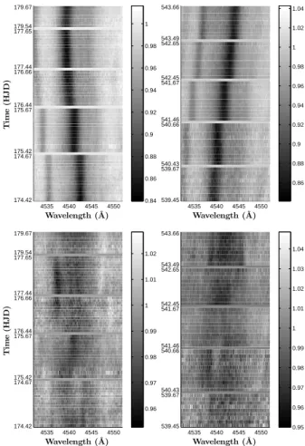
The variability of the He ii λ 4542 and N iii λλ 4511 – 4518 lines is less prominent than in the case of He i λ 4471. The raw dy-namic spectra of the He ii and N iii lines are dominated by the pri-mary’s orbital motion and do not reveal clear redwards-moving discrete depressions (see Fig. 4). The secondary dynamic spectra are qualitatively similar to those of He i λ 4471, but the variabil-ity is more subtle.
The power spectra averaged over the He ii λ 4542 line in the frame of reference of the secondary star can be described by the combination of the 0.82 and 1.65 d−1 frequencies and their aliases (see Fig. 5). For the 2010 data, a slightly cleaner
4535 4540 4545 4550 174.42 174.67 175.42 175.67 176.44 176.66 177.44 177.65 179.54 179.67 Wavelength (˚A) T im e (H J D ) 0.84 0.86 0.88 0.9 0.92 0.94 0.96 0.98 1 4535 4540 4545 4550 539.45 539.67 540.43 540.66 541.46 541.67 542.45 542.65 543.49 543.66 Wavelength (˚A) 0.86 0.88 0.9 0.92 0.94 0.96 0.98 1 1.02 1.04 4535 4540 4545 4550 174.42 174.67 175.42 175.67 176.44 176.66 177.44 177.65 179.54 179.67 Wavelength (˚A) T im e (H J D ) 0.96 0.97 0.98 0.99 1 1.01 1.02 4535 4540 4545 4550 539.45 539.67 540.43 540.66 541.46 541.67 542.45 542.65 543.49 543.66 Wavelength (˚A) 0.95 0.96 0.97 0.98 0.99 1 1.01 1.02 1.03 1.04
Fig. 4. Same as Fig. 2, but for the He ii λ 4542 line.
Table 2. Correspondence between the best frequencies (in d−1) found in this paper and those found by Mahy et al. (2011) in the CoRoT light curve.
Our Frequencies CoRoT Frequencies
0.37 0.368 0.399 (0.650) (1.646)
0.82 0.823 0.799
1.65 1.646 (0.650) (0.368) (0.399)
Notes. Photometric frequencies between brackets correspond to aliases due the 1-day aliasing that affects our time series.
prewhitening is achieved with 0.37 instead of 1.65 d−1, and for
the 2009 time series, a more efficient result is achieved including another harmonic frequency (2.47 d−1). Shifting the spectra into the frame of reference of the primary star essentially yields the same results.
Given the nitrogen overabundance of the primary star and the possible underabundance of the secondary reported by Linder et al. (2008), we expect a priori that the N iii lines should mainly be formed in the atmosphere of the primary star3. We have analysed
the two strongest N iii lines (λλ 4511 & 4515) in the frame of reference of the primary. The resulting power spectra are again explained by the 0.82 and 1.65 d−1frequencies and (in the 2009 data) some contribution at 0.37 d−1.
3
We note however that Fig. 1 reveals some shallow N iii absorptions also in the secondary spectrum.
A&A proofs: manuscript no. Plaskett 0 1 2 3 4 5 0 0.02 0.04 0.06 0.08 0.1 0 1 2 3 4 5 0 0.02 0.04 0.06 0.08 0.1 0 1 2 3 4 5 0 0.2 0.4 0.6 0.8 1 0 1 2 3 4 5 0 0.05 0.1 0.15 0.2 0 1 2 3 4 5 0 0.05 0.1 0.15 0.2 0 1 2 3 4 5 0 0.2 0.4 0.6 0.8 1
Fig. 5. Same as Fig. 3 but for the He ii λ 4542 secondary’s line. The prewhiten-ing in the middle panels was done with the 0.82 and 1.65 d−1frequencies.
4. Discussion
The analysis of our spectroscopic time series of Plaskett’s star in the previous section revealed three main frequencies 0.82, 1.65, and 0.37 d−1, although the properties of the latter two are
inter-dependent because of the aliasing problem. Before we discuss the possible interpretation of these results, let us first recall the ingredients of Plaskett’s star as (we think) we know this system. The primary star is a rather slow rotator presenting chemical en-richment indicating that it is most probably in a post-RLOF sta-tus. The secondary is a fast rotator probably surrounded by a flattened wind. The orbit is circular and the stars currently do not fill their Roche lobes. A magnetic field, probably associated with the secondary, was detected. This magnetic field could be at the origin of the flattened wind structure.
With these ingredients in mind, three scenarios could possi-bly explain the observed line profile variations: pulsations, tidal interactions, and an oblique magnetic rotator.
4.1. Pulsations
Mahy et al. (2011) tentatively assigned the 0.82 d−1frequency and its six harmonics to a low-order (2 ≤ l ≤ 4) non-radial pulsation (NRP). Our Fourier analyses provide us with the am-plitude (A) and the phase constant (ϕ0) of the variation as a
func-tion of wavelength. These quantities can help us test the NRP scenario. Indeed, for NRPs with moderate degrees l the phase constant usually changes monotonically across the line profile and the difference between the phase constant in the red wing and in the blue wing is directly related to the values of l and m of the pulsation (e.g. Schrijvers & Telting 1999, Zima et al. 2004).
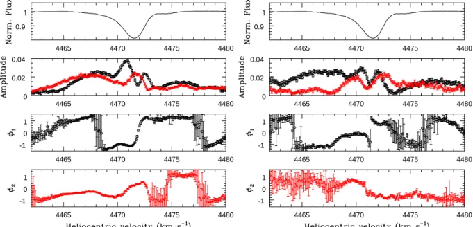
The amplitude and phase distributions of the 0.82 and 1.64 d−1frequencies of the He i λ 4471 secondary line are shown in Fig. 6. The uncertainties were evaluated via Monte Carlo sim-ulations (see Rauw et al. 2008). Whilst these distributions are possibly affected by the residuals of the primary line, they are quite erratic and do not ressemble what one would expect for typical NRPs.
If we consider the amplitudes and phase constants in the frame of reference of the primary, the variations are less erratic and, at least in the case of the 0.82 d−1frequency, are more
rem-iniscent of genuine NRPs. This would imply that the primary is responsible for the 0.82 and 1.65 d−1 frequencies. In the frame
of reference of the primary, significant amplitude of variability is found far away from the core of the primary line, out to −500
(-6.6 v sin i) and+400 km s−1(5.3 v sin i) away from the line
cen-tre. Similar results are obtained for the He ii λ 4542 line. Variabil-ity over such an extended wavelength range around the line core is however rather unexpected for conventional NRPs in a slow rotator, therefore suggesting that the observed variability is most likely associated with the secondary star. The apparent variabil-ity of the primary could then be induced by travelling features of the much broader secondary line when they cross the position of the primary line.
4.2. Tidal interactions
The analysis of the line profile variations in the slightly eccentric binary system Spica (Palate et al. 2013 and references therein) has shown that tidal interactions could explain Spica’s line pro-file variations. Although Plaskett’s star is not an eccentric sys-tem, the non-synchronicity of the secondary rotation could lead to tidally induced variations such as those reported by Moreno et al. (2005). Therefore, we can wonder whether tidal interactions could be responsible for the variations reported hereabove.
We have thus tried to model Plaskett’s star with the TIDES code (see Moreno et al. 1999, 2005, 2011) combined to CoM-BiSpeC4 (see Palate & Rauw 2012 and Palate et al. 2013). The TIDES code computes the time-dependent shape of the stellar surface for eccentric and/or asynchronous systems accounting for centrifugal and Coriolis forces, gas pressure, viscous effects and gravitational interactions. From that, CoMBiSpeC computes the synthetic spectra of the stars at several orbital phases.
We stress that our goal here is not to fine tune the parameters that reproduce perfectly the spectra of the components of Plas-kett’s star and their observed variations. Here, we rather wish to test whether or not tidal interactions can produce detectable variations in the spectra of this system. Indeed, fitting the spec-tra rigorously is a challenging task because of a large number of free/unknown parameters and the non-solar composition of the stars (see Linder et al. 2008); CoMBiSpeC currently only works with atmosphere models that have a solar composition. In the present paper, we have only adjusted the temperatures to repro-duce the observed strength of the He i λ 4471 and He ii λ 4542 lines. The parameters used are listed in Table 3.
Mahy et al. (2011) suggested that the frequencies near 0.4 d−1could correspond to the rotational frequency of the
sec-4 TIDES: tidal interaction with dissipation of energy through shear. CoMBiSpeC: code of massive binary spectral computation.
4465 4470 4475 4480 0.98 0.99 1 1.01 4465 4470 4475 4480 0 0.02 0.04 4465 4470 4475 4480 -1 0 1 4465 4470 4475 4480 -1 0 1 4465 4470 4475 4480 0.98 0.99 1 1.01 4465 4470 4475 4480 0 0.02 0.04 4465 4470 4475 4480 -1 0 1 4465 4470 4475 4480 -1 0 1
Fig. 6. Amplitude and phase variations for the He i λ 4471 line in the frame of reference of the secondary during the 2009 (left) and 2010 (right) campaigns. Two frequencies have been considered simultaneously: ν1= 0.82 and ν2= 1.65 d−1. The top panels yield the mean secondary profile, whilst the amplitudes associated with the two frequencies are shown in the second panels. The two lower panels indicate the phase constants of these frequencies. 4465 4470 4475 4480 0.9 1 4465 4470 4475 4480 0 0.02 0.04 4465 4470 4475 4480 -1 0 1 4465 4470 4475 4480 -1 0 1 4465 4470 4475 4480 0.9 1 4465 4470 4475 4480 0 0.02 0.04 4465 4470 4475 4480 -1 0 1 4465 4470 4475 4480 -1 0 1
Fig. 7. Same as Fig. 6, but in the frame of reference of the primary.
ondary. The projected equatorial rotational velocity of the sec-ondary has been evaluated to ∼ 300 km s−1by Linder et al. 2008. These authors also derived a log g equal to 3.5 ± 0.1. Adopting an inclination of 67◦ as proposed by Mahy et al. (2011), and considering that the rotation frequency is 0.4 d−1, the projected
rotational velocity of 300 km s−1 yields a radius R = vrot
2 π νrot of 16.1 R for the secondary. The log g and minimum mass of the
secondary (mS sin3i= 47.3 M , Linder et al. 2008) along with
the adopted inclination of 67◦(Mahy et al. 2011) rather suggest
a radius5 of 20.7+1.3
−2.2 R . In this latter case, the projected
rota-tional velocity would be equal to ∼ 385 km s−1. The discrepancy between these rotational velocities can be explained by several
5 The latter was determined from the relation g= GM
R2 (1 −Γ) where Γ accounts for the radiation pressure of the star.
factors: the uncertainties on the inclination (Mahy et al. 2011 indicated a range from 30 to 80◦), the error on the rotational ve-locity determination, on the log g, and on the frequency.
Our simulations indicate that tidal interactions can produce visible variations in the lines of the secondary. Because the pri-mary is thought to be in synchronous rotation in a circular or-bit, it is expected that there is no variability of the primary due to tidal interactions. The strength of the simulated variations is comparable to the observed ones. Reducing the secondary radius to 18 R slightly lowers the amplitude of the tidally induced
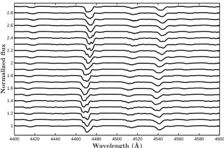
vari-ations, although they remain well visible in the synthetic spec-tra. Fig. 8 displays the simulated line profile variations in the secondary during the orbital cycle. Whilst our code cannot sim-ulate the impact of the tidal interactions on a co-rotating con-fined wind, it seems very plausible that the tidal interactions also
A&A proofs: manuscript no. Plaskett Table 3. Parameters used for simulation with the TIDES+ CoMBiSpeC
model.
Parameters Primary Secondary
Period (day) 14.396 Eccentricity 0 Inclination (◦) 67 Mass (M ) 58.2 60.6 Polar temperature (K) 33000 32000 Polar radius (R ) 20.0 20.7 Polar log(g) (cgs) ' 3.5 ' 3.5 vrot(km s−1) 70.3 296 v sin i (km s−1) 64.7 273 β(a) 1.0 4.12 Viscosity, ν (R 2d−1) 0.028 0.035 Layer depth (∆R/R) 0.07 0.07 Polytropic index 1.5 1.5
Number of azimuthal partitions 500 500 Number of latitudinal partitions 20 20
Notes. (a)The β parameter measures the asynchronicity of the star at periastron and is defined by β = 0.02Pvrot
R ×
(1−e)3/2
(1+e)1/2, where vrotis the equatorial rotation velocity, R is the equilibrium radius, and e is the eccentricity.
affect the latter and thus extend into the emission humps. This re-sult brings up the interesting possibility that breaking tidal waves near the secondary’s equator could produce an enhanced mass-loss in this region (see Osaki 1999). Combined with wind con-finement due to the magnetic field (Grunhut et al. 2013a, 2013b), this effect could produce the equatorial torrus of circumstellar material that was advocated by Wiggs & Gies (1992) and Linder et al. (2006, 2008). The much smaller radius (10.7 R ) proposed
by Grunhut et al. (2013a) not only fails to reproduce the log g value inferred from the model atmosphere code fits (see below), but would also considerably reduce the amplitude of surface os-cillations due to tidal interactions.
We have performed a Fourier analysis of the individual sim-ulated spectra of the secondary stars. The power spectrum dis-plays a peak at the secondary’s rotation frequency imposed in the model, but does not show peaks at the harmonic frequen-cies. Tidal interactions can thus induce profile variations, pro-vided the stellar radii are sufficiently large. However, the current model does not explain the full frequency content of HD 47129’s spectroscopic and photometric variations.
4.3. Magnetically confined winds
Grunhut et al. (2013a) reported on the discovery of a magnetic field in Plaskett’s star with a minimum surface dipolar strength of 2.8 kG at the magnetic poles. Such a strong magnetic field could confine the secondary’s stellar wind, thereby producing the emission humps seen around the He i λ 4471 line as well as the double-peaked Hα emission. Using additional spectropolari-metric observations, Grunhut et al. (2013b) inferred a tilt angle of the magnetic axis of (80 ± 5)◦ with respect to the rotation axis. This would result in a magnetic configuration very simi-lar to HD 57682 (Grunhut et al. 2012). One would then expect a double-wave modulation of the strength of the emission features. Based on a periodicity search in the variations in the Hα equiv-alent width and the longitudinal magnetic field, Grunhut et al.
4400 4420 4440 4460 4480 4500 4520 4540 4560 4580 4600 1 1.2 1.4 1.6 1.8 2 2.2 2.4 2.6 2.8 N o rm a li z e d fl u x Wavelength (˚A)
Fig. 8. Line profile variations in the synthetic spectra of the secondary during the orbital cycle. The spectra (separated by 0.05 in phase) have been shifted vertically by 0.1 continuum unit for clarity.
(2013b) inferred a rotational period of 1.215 d for the secondary, corresponding to the 0.82 d−1frequency.
This scenario could thus explain our detection of the 0.82 and 1.65 d−1frequencies quite naturally in the emission humps.
However, adopting 0.82 d−1 as the secondary’s rotational fre-quency would lead to a radius estimate from the projected rota-tional velocity that is twice smaller than what we have obtained above, thus enhancing the discrepancy between the radius esti-mated from v sin i and the one estiesti-mated from log g.
Concerning the latter discrepancy, we note that Wiggs & Gies (1992) previously reported a 2.78 d period in the equiva-lent width of the Hα emission wings6.
4.4. Summary and conclusion
Our analysis of the He i λ 4471, N iii λλ 4510-4518, and He ii λ 4542 lines of Plaskett’s star revealed variations at several fre-quencies: 0.37, 0.82, and 1.65d−1. The strongest variations are
found for the He i line.
Considering the current knowledge of the system, it is diffi-cult to assign the spectroscopic variability to either the primary or the secondary star. Indeed, our analysis yielded conflicting results in this respect: whilst the velocity range over which vari-ations are detected clearly favours the secondary star, the pattern of the amplitude and phase of the variations makes more sense if they originate in the primary star. As a result, none of the current scenarios (pulsations, tidal interactions, magnetically confined winds) accounts for all the aspects of the observed variations.
Acknowledgements. We would like to thank Pr. G. Koenigsberger who provided us with the TIDES code and helped us to use it. We are grateful to the referee, Dr. Jason Grunhut who helped us improve this paper. We acknowledge support through the XMM/INTEGRAL PRODEX contract (Belspo), from the Fonds de Recherche Scientifique (FRS/FNRS), as well as by the Communauté Française de Belgique - Action de recherche concertée - Académie Wallonie - Europe.
6 Wiggs & Gies 1992 suggested an origin in the winds of the stars, corresponding to a frequency of 0.36 d−1 in good agreement with the 0.37 d−1rotation frequency suggested by Mahy et al. (2011). A corollary would be that the variations in the longitudinal magnetic field presented by Grunhut et al. (2013b) would probably have to be interpreted as due to a more complex magnetic field than a simple dipole.
References
Auvergne, M., Bodin, P., Boisnard, L., et al. 2009, A&A, 506, 411
Baglin, A., Auvergne, M., Barge, P., et al. 2006, in ESA SP, ed. M. Fridlund, A. Baglin, J. Lochard, & L. Conroy, 1306, 33
Bagnuolo, W.G.Jr., Gies, D.R., & Wiggs, M.S. 1992, ApJ, 385, 708 González, J. F., & Levato, H. 2006, A&A, 448, 283
Gosset, E., Royer, P., Rauw, G., Manfroid, J., & Vreux, J.-M. 2001, MNRAS, 327, 435
Grunhut, J.H., Wade, G.A., Sundqvist, J.O., et al. 2012, MNRAS 426, 2208 Grunhut, J.H., Wade, G.A., Leutenegger, M., et al. 2013a, MNRAS, 428, 1686 Grunhut, J.H., Wade, G.A., and the MiMeS Collaboration 2013b, in Setting
a New Standard in the Analysis of Binary Stars, eds. K. Pavlovski, A. Tkachenko, & G. Torres, EAS Publication Series, 64, 67
Heck, A., Manfroid, J., & Mersch, G. 1985, A&AS, 59, 63 Hillier, D.J., & Miller, D.L. 1998, ApJ, 496, 407
Linder, N., Rauw, G., Pollock, A.M.T., & Stevens, I.R. 2006, MNRAS, 370, 1623
Linder, N., Rauw, G., Martins, F., et al. 2008, A&A, 489, 713 Mahy, L., Gosset, E., Baudin, F., et al. 2011, A&A, 525, 101 Moreno, E. & Koenigsberger, G. 1999, RMA&A, 35, 157
Moreno, E., Koenigsberger, G. , & Toledano, O. 2005, A&A, 437, 641 Moreno, E., Koenigsberger, G., & Harrington, D. M. 2011, A&A, 528, 48 Osaki, Y. 1999, in Variable and Non-spherical Stellar Winds in Luminous Hot
Stars, IAU coll. 169, eds B. Wolf, O. Stoll, & A.W. Fullerton, Lecture Notes in Physics 523, 329
Palate, M., & Rauw, G. 2012, A A, 537, 119
Palate, M., Koenigsberger, G., Rauw, G., Harrington, D., & Moreno, E. 2013, A&A, 556, 49
Palate, M., Rauw, G., Koenigsberger, G., & Moreno, E. 2013, A&A , 552, 39 Plaskett, J.S. 1922, JRASC, 16, 284
Rauw, G., De Becker, M., van Winkel, H., et al. 2008, A&A, 487, 659 Rudy, R.J., & Herman, L.C. 1978, PASP, 90, 163
Schrijvers, C., & Telting, J.H. 1999, A&A, 342, 453 Wiggs, M.S., & Gies, D.R. 1992, ApJ, 396, 238