Rio de Janeiro, Brazil, September 8 - 10, 2010
ROBUSTNESS OF STEEL AND COMPOSITE BUILDINGS
UNDER IMPACT LOADING
Ludivine Comeliau, Jean-François Demonceau and Jean-Pierre Jaspart
Liège University, ArGEnCo Department
e-mails: ludivine.comeliau@ulg.ac.be, jfdemonceau@ulg.ac.be, jean-pierre.jaspart@ulg.ac.be
Keywords: Robustness, Building frames, Column impact, Dynamic effects.
Abstract. In case of a vehicle impact against a building frame, one or more columns may be damaged or even fully destroyed. In such an exceptional event, the risk of progressive collapse of the whole structure has to be mitigated. Several approaches potentially exist to face this problem. In the present study, the so-called alternative load path method is followed. In two recent PhD studies at Liège University, a complete analytical procedure was developed permitting the prediction of the structural response of steel or composite plane frames further to the loss of a column. For sake of simplicity, these first works were based on the assumption of static behaviour. More recently, complementary research was carried out with the objective to address the dynamic effects. As a result, an original procedure for the appraisal of the structural robustness of plane building frames was proposed. The present paper presents this work. 1 INTRODUCTION
The loss of a column in a building frame may be associated with different types of exceptional events: explosion, impact of a vehicle, fire... Amongst these actions, some induce negligible dynamic effects; then a “static” response can be assumed. However, in many other circumstances, the column is removed relatively quickly, which induces significant dynamic amplifications that need to be taken into account.
Investigations were conducted at Liège University in the last few years regarding the static behaviour of two-dimensional building frames suffering the loss of a column further to an unspecified accidental event. These studies are detailed in two PhD theses: the thesis of Demonceau [1] and the thesis of Luu [2]. They resulted in the development of simplified analytical methods for the prediction of the structural response assuming static behaviour. The dynamic response of building frames further to the loss of a column was more recently investigated by Comeliau [3]. In particular, the behaviour of a simplified substructure was studied. In this paper, researches conducted in [3] are summarized and the main results are reflected.
2 GLOBAL APPROACH AND PREVIOUS RESEARCHES
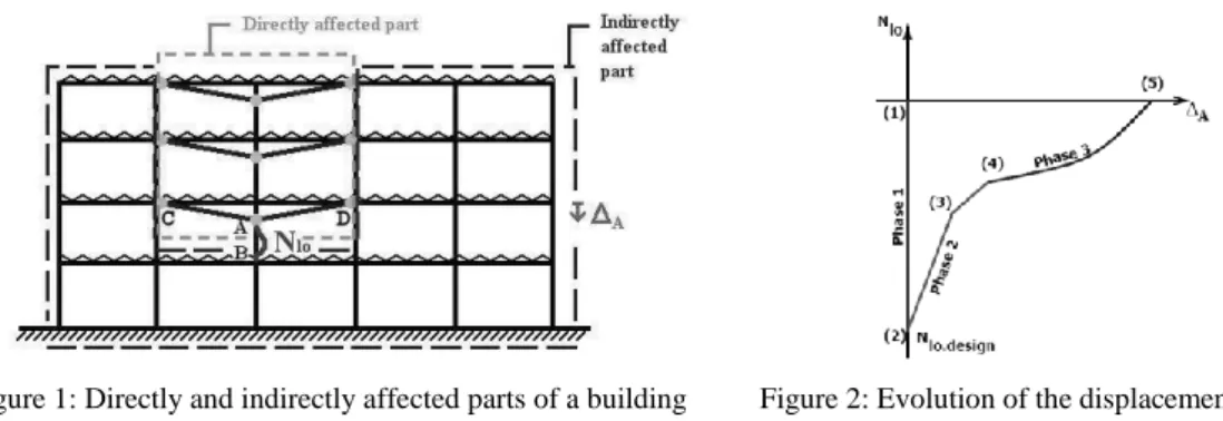
The approach followed in [1] and [2] to study the static response of a structure losing a column is based on a decomposition of the latter in two parts: the directly affected part, which is made up of the beams and columns above the lost column; and the indirectly affected part, which consists of the rest of the frame (Figure 1).
The evolution of the vertical displacement at the top of the failing column versus the axial load that it supports is represented by a curve as illustrated in Figure 2. The behaviour can be divided in three main phases. The first one corresponds to the application of the “normal” loads on the structure. It goes from point (1) (unloaded, ) to point (2) (conventional loading, ). The structure is assumed to remain elastic during this phase. At point (2), the exceptional event occurs; then the column “AB” is progressively removed: the compression it sustains starts to decrease. During phase 2, the directly
affected part goes from a fully elastic behaviour to a plastic mechanism. The first plastic hinge appears at point (3) while the complete plastic mechanism is formed at (4). After point (4), rapidly increases and second order effects become important. In particular, significant catenary actions develop in the bottom beams of the directly affected part, which makes the system stiffness increase and the deformation rate decrease. If the frame exhibits sufficient robustness, a final stable state is obtained at (5), when .
Obviously, it is only possible to reach a final stable state, corresponding to point (5), if no failure occurs prematurely, would it be in the directly affected part or in the rest of the structure; i.e. it is necessary that: (i) the loads transferred from the directly affected part to the indirectly affected part do not induce the collapse of elements in the latter, (ii) the compression supported by the upper beams of the directly affected part due to an “arch effect” do not lead to their buckling, (iii) the different structural elements of the directly affected part exhibit sufficient resistance and ductility to reach the displacement
. In some cases, the column may be completely removed ( ) before reaching phase 3.
The response of the structure at phases 1 and 2 was investigated in [2] while phase 3 was studied in [1]. During this last phase, the global plastic mechanism is formed in the directly affected part and large displacements are observed. As a consequence, second order effects become significant. In particular, tension loads develop in the bottom beams of the directly affected part. It was shown that the membrane forces developing in the two beams overhanging directly the lost column (“CA” and “AD” in Figure 1) are significantly more important than the ones developing in the other beams. That is why it was decided to investigate the behaviour of this single storey and thus to extract from the frame a simplified substructure consisting of this double-beam and its beam-to-column joints (Figure 3). The influence of the indirectly affected part is characterised by an elastic horizontal spring having a stiffness K and a resistance . Analytical methods aiming to estimate the value of these parameters K and were developed in [2]. The ability of such a substructure to simulate with sufficient accuracy the behaviour of the directly affected part was validated by numerical tests [1]. Finally, an analytical approach was developed to predict the response of the frame during phase 3 [1], on the basis of the “substructure approach”. So, the static curve ( , ) can be entirely derived from the combination of the developments detailed in [1] and [2], which provides a global analytical procedure. However, it is only valid as long as a static response of the frame is observed.
Figure 3: Double-beam simplified substructure
Figure 2: Evolution of the displacement versus the axial load Figure 1: Directly and indirectly affected parts of a building
3 DYNAMIC BEHAVIOUR OF A SUBSTRUCTURE 3.1 Description of the considered substructure and loading
The dynamic behaviour of a simplified substructure such as described above was investigated under the following hypothesis: steel structures are considered, the behaviour law is admitted to be independent of the strain rate and a quasi-static elastic-perfectly plastic law is assumed (infinite ductility), the stiffness K of the lateral spring remains constant, the beam-to-column joints are perfectly rigid and fully resistant.
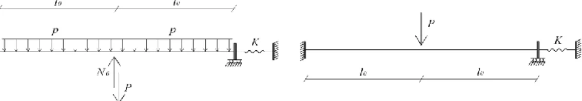
A uniformly distributed load is applied on the double-beam. Initially, the central support is present and sustains a force ( , being the initial length of each beam). Then, the latter is progressively removed, which is simulated by the application of a force equal and opposite to in the middle of the system. The complete loss of the support takes a time and a linear decrease of the force it sustains is assumed. In static conditions, it had been shown in [1] that the uniformly distributed load could be neglected as far as the behaviour in phase 3 was investigated, i.e. for greater than , which is the force corresponding the plastic plateau in the static curve (development of a beam mechanism). The validity of this assertion for dynamic situations was studied [3]. Many numerical dynamic tests were made on a substructure in order to compare the maximum displacement obtained in the two loading situations (Figure 4) for the same loading parameters and . It was observed that the difference is limited provided the force P is great enough (above the static plastic plateau). That is the reason why the behaviour of the substructure under the simplified loading situation was mainly investigated. Moreover, it was shown that the introduction of damping in the system does not induce a significant decrease of the maximum displacement [3]. As a consequence, undamped systems were considered; this constitutes a conservative approach.
Figure 4: Considered system with realistic and simplified loadings
Figure 5: Time evolution of the applied force P(t)
3.2 Influence of different parameters on the dynamic behaviour
To investigate the dynamic response of the substructure, a simplified loading is considered, consisting of a single concentrated load applied in the middle of the system. Obviously, as well as in static, the level of the load and the geometrical and mechanical characteristics of the structure have an influence on its behaviour. In case of dynamic loadings, the application rate of , characterised by the rise time (Figure 5), is also important. Besides, mass and damping properties are essential factors on which the dynamic response depends.
As mentioned above, the studied systems are undamped ones. As far as mass influence is concerned, a change in mass has first the effect of modifying the principal natural period of the system. Numerical tests proved that the dynamic response of a given structure is actually governed by two parameters: and
, where is the period of the principal eigenmode in elastic domain [3]. Thus, if the mass of the system is modified but the rise time of the load is adapted so that the ratio is kept constant, then the maximal displacement remains unchanged. Furthermore, the time evolution of the displacement remains the same provided it is expressed as a function of a non-dimensional time (or ).
In [3], the behaviour of the substructure according to the loading parameters and (or ) was investigated through numerical dynamic analyses. All the results presented below are related to the following particular substructure:
beams: , IPE 450, S235, ( ;
spring: stiffness , resistance
Performing dynamic analyses for different loading conditions ( , ) and registering the maximum
displacement obtained for each one, curves giving as a function of the applied force were
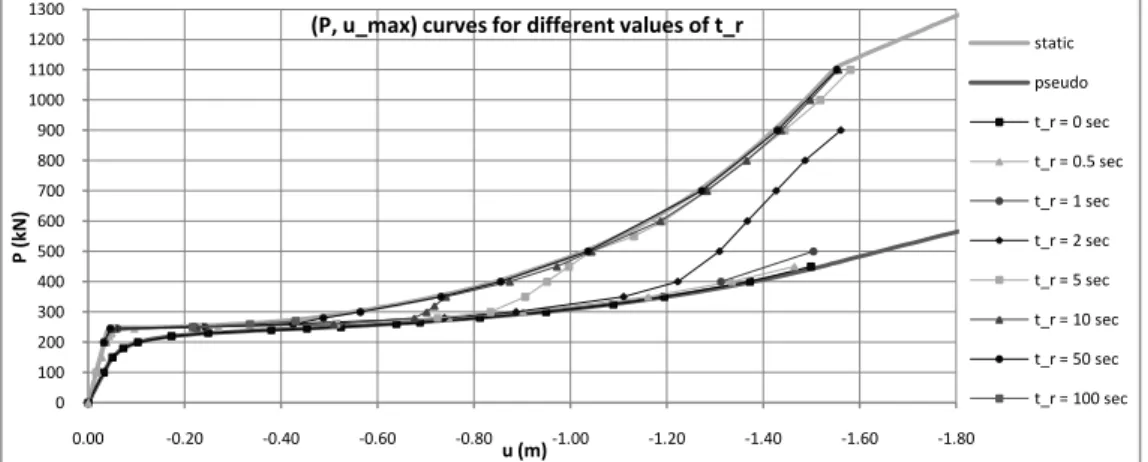
established, for different values of (constant along one curve). These curves are drawn in Figure 6; only dynamic loadings leading to smaller than the displacement corresponding to the complete yielding of the beams in tension are considered. On this graph, the upper curve is the static one, while the lower curve is the so-called pseudo-static one, which gives the maximum displacement reached if is applied instantaneously ( ). Such a curve can easily be established provided only the nonlinear static curve is known, following a procedure developed at London Imperial College [4]. Obviously, the maximum displacement corresponding to a force will always be situated between the static
displacement ( ) and the displacement caused by the sudden application of the load ( ). As a
consequence, every ) curve will lie between the static and the pseudo-static ones all along, for any value of . As a general rule, for a given value of , tends to decrease when increases.
Figure 6: Maximal dynamic displacement according to the value of the load and its rise time
Different types of behaviour can already be highlighted from Figure 6. For loads , two types
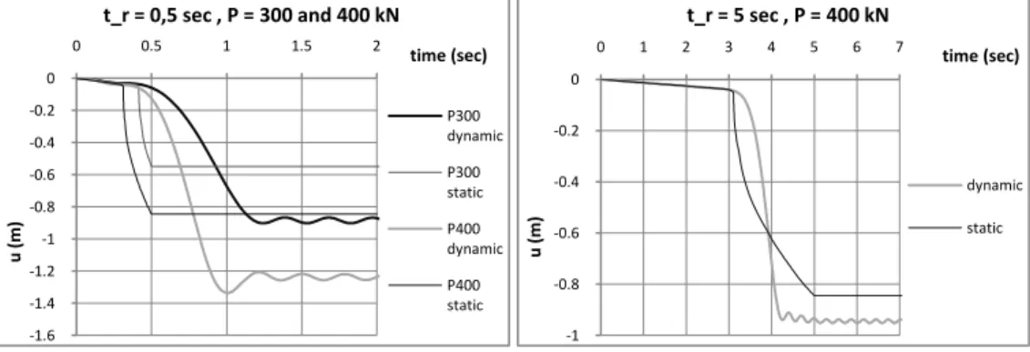
of response are observed according to the loading parameters and . For the first type, the maximum dynamic displacement is greater than the static displacement while, for the second one, is very close to . Examples of both response types are presented below. For each of them, the dynamic curve representing the time evolution of the displacement is compared to the static curve , which represents the evolution of the displacement, dynamic amplification being neglected. Accordingly,
is the static displacement associated with the value of the applied load at the time . A response of type 1 (Figure 7) is met when the system yields and gets beyond the static displacement corresponding to the final load . Then, it finally oscillates around a value of the displacement greater than this static displacement. If a behaviour of type 2 occurs (Figure 8), then, when the plastic mechanism forms and the displacement suddenly increases, the latter however remains smaller than the static displacement corresponding to the final force . Next, the dynamic curve oscillates around a
0 100 200 300 400 500 600 700 800 900 1000 1100 1200 1300 -1.80 -1.60 -1.40 -1.20 -1.00 -0.80 -0.60 -0.40 -0.20 0.00 P (kN) u (m)
(P, u_max) curves for different values of t_r
static pseudo t_r = 0 sec t_r = 0.5 sec t_r = 1 sec t_r = 2 sec t_r = 5 sec t_r = 10 sec t_r = 50 sec t_r = 100 sec
more or less constant value whilst the applied load continues to rise. Once the force has increased enough so that the associated static displacement meets the dynamic displacement, the latter starts to increase again, oscillating around the static curve. Eventually, the maximum dynamic displacement is close to
Figure 7: Examples of the time evolution of the displacement for a response of type 1
Figure 8: Examples of the time evolution of the displacement for a response of type 2
The time evolution of the displacement for both response types can be explained as follows. When the plastic mechanism forms, the displacement rapidly increases and a distinct change in the slope of the curve is observed. However, due to its inertia, the system gets on the move progressively and the displacement remains at the beginning below the static displacement corresponding to the applied load . The system starts to accelerate and the dynamic displacement gets closer to the static one. Then it exceeds the latter and, the displacement of the system becoming higher than the static displacement associated with the force applied at the considered time, the velocity begins to decrease. The reduction of the velocity to zero, which corresponds to the first maximum of the dynamic displacement curve and a “stabilisation” of the system, may occur for a displacement smaller or greater than the static displacement associated with the final load; that is what distinguishes the two behaviour types. Then, there is a sort of plateau in the curve . In the first case (type 1), this plateau is infinite. In the second case (type 2), it carries on until the applied force has sufficiently increased so that the corresponding static displacement is equal to the dynamic displacement. Next, the dynamic curve oscillates around the static one to finally stabilize around a value of the displacement close to .
As far as internal forces are concerned, the axial load in the beams remains very small before the appearance of the three plastic hinges. When the moment in the middle and at the extremities of the
-1.6 -1.4 -1.2 -1 -0.8 -0.6 -0.4 -0.2 0 0 0.5 1 1.5 2 u (m ) time (sec) t_r = 0,5 sec , P = 300 and 400 kN P300 dynamic P300 static P400 dynamic P400 static -1 -0.8 -0.6 -0.4 -0.2 0 0 1 2 3 4 5 6 7 u (m ) time (sec) t_r = 5 sec , P = 400 kN dynamic static -1.6 -1.4 -1.2 -1 -0.8 -0.6 -0.4 -0.2 0 0 2 4 6 8 10 12 u (m ) time (sec) t_r = 10 sec , P = 450, 700 and 1000 kN P450 dynamic P450 static P700 dynamic P700 static P1000 dynamic P1000 static
double-beam reaches the plastic value , the mechanism forms and the displacement rapidly increases, which induces the development of significant membrane forces in the beams. As a consequence, the moment acting in the plastic hinges decreases to respect the M-N plastic interaction relation. At the end, oscillations of M and N are observed while the displacement is oscillating around a constant value. The amplitude of the oscillations of the tension force is limited as the amplitude of the variations of the displacement is also small. On the other hand, the moment varies more importantly, in phase with the oscillations of . There corresponds a succession of elastic “unloadings-loadings” that can be observed on the M-N interaction diagram as well as on the M-u and N-u curves [3]. Moreover, it is interesting to note that the maximum axial load in the beams, which is obtained when is reached, is the same as the tension force that would develop if this displacement was reached statically. Accordingly, this membrane force can be deduced from the sole knowledge of and the static response.
3.3 Simplified approach to estimate the maximum dynamic displacement
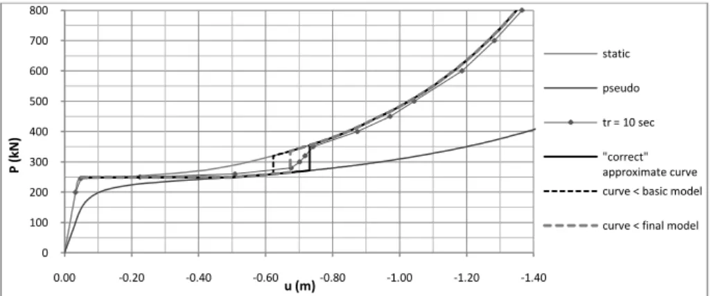
The objective was to develop a simplified method to estimate the maximum displacement reached for given loading conditions ( , ) with . Then, it would be possible to predict the required deformation capacity of the structural members as well as the tension force they should resist. In view of the aspect of the ( , ) curves (see Figure 6), the idea was to approach the latter, beyond the plastic plateau, by approximate curves established as follows [3]: section 1 horizontal at the level of ; section 2 pseudo-static curve; section 3 vertical between the pseudo-static and the static curve, at the
abscissa at which the actual ( , ) curve joins the static curve; section 4 static curve.
An example of such a curve is presented in Figure 9 (“correct” approximate curve). For too low values of the ratio , the dynamic curve does not join the static one and sections 3 and 4 cannot be defined. It is also possible that section 2 does not exist.
Figure 9: Example of an approximate dynamic curve
To be able to draw such an approximate curve, the value of is still to determine. The point at which the dynamic curve ( , ) associated with a given value of joins the static curve corresponds to a transition between the two types of response previously described. Indeed,
we have > for (type 1) and for (type 2). As explained
before, the behaviour type is governed by the value of the displacement ( ) when the velocity is
reduced to zero for the first time after the formation of the plastic mechanism. In fact, type 1 corresponds
to while type 2 is associated with .
As a consequence, if could be evaluated for a given loading, then the approximate dynamic
curve corresponding to a fixed value of (or ) could be established following this
procedure: (i) determination of the displacement for different values of and comparison with
the static displacement ; (ii) identification of the force for which : this value
0 100 200 300 400 500 600 700 800 -1.40 -1.20 -1.00 -0.80 -0.60 -0.40 -0.20 0.00 P (kN) u (m) static pseudo tr = 10 sec "correct" approximate curve curve < basic model curve < final model
of the load is ; (iii) deduction of from the static curve; (iv) drawing of the
complete curve . In order to carry out the first stage of this procedure, a simplified model
was developed to estimate [3]. The latter is described below.
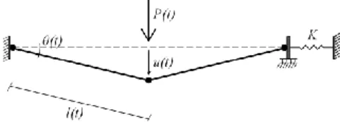
At first, a basic simplified model was developed under the following assumptions. It is a rigid-plastic model, in which the beams are considered to be infinitely rigid and thus keeping a constant length .
The plastic hinges developing at their extremities are submitted to a moment admitted constant,
interaction with the axial load being neglected. Finally, moderate displacements are supposed, which means that:
( )
Figure 10: Considered system and main definitions An energy equation was written, consisting in expressing that the work done by the external force is equal to the sum of the kinetic energy, the work of the plastic hinges and the energy stocked in the lateral spring:
(1)
(2)
Where is the generalised mass of the system, is the elongation of the
horizontal spring and the force it sustains.
This equation is only valid until the first maximum of the displacement is reached, which is ,
and provided it occurs before the applied load become constant, so that it is expressed as .
However, these restrictions are of no consequence here. Indeed, what we are interested in is the
determination of and what happens after is no concern. Moreover, as the final objective is the
determination of , only responses relatively close to the intermediate situation between the two behaviour types are interesting; and, in such cases, the plateau always starts at a time . In order to resolve the previous equation, initial conditions have to be defined. In the considered rigid-plastic system, the displacement and the velocity are both zero until the plastic mechanism is formed. So the
equation is resolved from the time , with the initial conditions: and .
Figure 11: Typical response of the system defined on the basis of the model
Unfortunately, this equation has no analytical solution and had to be numerically resolved. Moreover, it was observed that the use of this basic model leads to underestimate , and then the value of (see the corresponding curve on the graph of Figure 9). That can be explained by the fact that different aspects neglected in the development of the basic model would induce greater displacements if
taken into account. Eventually, the final model was developed from equation (1) but considering the M-N
plastic interaction ( ) and the elongation of the beams ( ). Then,
the last approximate curve of Figure 9 was drawn using this final model and following the previously described procedure. It is observed that the developed simplified method still leads to underestimate the
extreme dynamic displacement for values of the force close to . For the considered example, the
maximum unsafe error is about 8%.
4 CONCLUSION AND PERSPECTIVES
Within the present paper, part of the research carried out in [3] is reflected. As an introduction, a general approach developed at Liège University to study the behaviour of building frames further to the loss of a column was first presented, as well as previous works performed on the static response of such frames ([1] and [2]). In particular, the possibility to define a substructure able to reproduce the global response of a frame when membrane effects develop further to a column loss was illustrated.
Then, some investigations conducted in [3] were introduced. The latter are mainly dedicated to the study of the dynamic response of the previously defined substructure further to the loss of its central support. The time evolution of the displacement, yielding and internal forces was studied in detail through numerical simulations; the influence of different properties of the structure (mainly its first period ) and of its loading conditions (the value of the load initially sustained by the central support and the duration of its removal) was highlighted. Finally, a simplified method was proposed to quantify the maximum
dynamic displacement suffered by a substructure under a given loading ( ).
Of course, it would be interesting to refer to these developments in the case of an actual building frame; in the same way as, in static conditions, such a simplified substructure is able to reproduce the response of the whole frame. The dynamic behaviour of building frames further to the loss of a column was studied [3]. Qualitatively, it showed many similarities with the response of a substructure in terms of displacement, yielding and internal forces. However, the ability of the extracted substructure to reflect the dynamic behaviour of the whole frame should be investigated in more depth.
A second perspective concerns the improvement of the simplified model. Indeed, the proposed procedure aiming to predict the maximum dynamic displacement may lead to underestimate the latter. This method was validated for few study cases, with maximum unsafe errors of about 10%, which is reasonable. However, the number of tests is too small to draw general conclusions. Besides, the equation of the model has no analytical solution and has to be numerically solved. As the objective at Liège University is to come at the end with easy-to-apply simplified analytical methods, it would be interesting to establish an approximate solution of the model equation, having an analytical expression.
In conclusion, the presented investigations constitute a first step for the implementation of the dynamic effects within the general concept developed in Liège and already validated in static. Further studies are planned in a near future.
REFERENCES
[1] J.F. Demonceau. “Steel and composite building frames: sway response under conventional loading and development of membrane effects in beams further to an exceptional action”. PhD thesis presented at Liège University. Belgium, 2008.
[2] H.N.N. Luu. “Structural response of steel and composite building frames further to an impact leading to the loss of a column”. PhD thesis presented at Liège University. Belgium, 2008.
[3] L. Comeliau. “Effets du comportement dynamique des structures de bâtiments en acier suite à la ruine accidentelle d’une colonne portante”. Travail de fin d’études, Université de Liège. Belgique, 2009. http://hdl.handle.net/2268/32284
[4] A.G. Vlassis. “Progressive collapse assessment of tall buildings”. Thesis submitted in fulfilment of the requirements for the degree of Doctor of Philosophy of the University of London and the Diploma of Imperial College London. UK, April 2007.