IMPACTS OF DISTRICT METERED AREAS IMPLEMENTATION ON WATER QUALITY IN A FULL-SCALE DRINKING WATER DISTRIBUTION SYSTEMS
VANESSA CRISTINA DIAS
DÉPARTEMENT DES GÉNIES CIVIL, GÉOLOGIQUE ET DES MINES ÉCOLE POLYTECHNIQUE DE MONTRÉAL
THÈSE PRÉSENTÉE EN VUE DE L’OBTENTION DU DIPLÔME DE PHILOSOPHIAE DOCTOR
(GÉNIE CIVIL) AOÛT 2016
ÉCOLE POLYTECHNIQUE DE MONTRÉAL
Cette thèse intitulée :
IMPACTS OF DISTRICT METERED AREAS IMPLEMENTATION ON WATER QUALITY IN A FULL-SCALE DRINKING WATER DISTRIBUTION SYSTEMS
présentée par : DIAS Vanessa Cristina
en vue de l’obtention du diplôme de : Philosophiae Doctor a été dûment acceptée par le jury d’examen constitué de :
M. BARBEAU Benoit, Ph. D., président
Mme PRÉVOST Michèle, Ph. D., membre et directrice de recherche Mme DORNER Sarah, Ph. D., membre
DEDICATION
In memory of my beloved father
ACKNOWLEDGEMENTS
I think I’m a very lucky person to have in my life so special family and friends who believe and support me no matter what. Since I have moved to Canada to pursue my doctoral studies and research I had the opportunity to meet so many other interesting people from different cultures I was not used to. Just like people who are already part of my life, these new people I met were very significant and marked me over my long way, sometimes with a simple look, word or smile. First, I would like to thank my advisor, Dr. Michèle Prévost, for accepting me as her student at the Industrial Chair in Drinking Water and for trusting me this project. I really appreciate every moment we spent together planning the work and discussing the results. Every time we met in her office I left very stimulated and energized because of her dynamism, openness, and positive attitude. I remember the first time I wrote her looking for a mentor, when she was on sabbatical in Australia. Oddly enough, at the end of this cycle she is again on sabbatical, again in Australia. Once more, thank you for giving me the opportunity to be part of your team and help me in my professional development.
I would also like to thank Dr. Marie-Claude Besner. She was my co-advisor in the beginning of this research but she left the research in the university to work as a research and development engineer for the city of Montreal. Thank you Marie-Claude for your comments, suggestions and to be part of the foundation of this research. In the course of this project I sometimes regretted that you were no longer part of it.
I would like to express my gratitude to the city of Montreal for allowing us to be part of this great project concerning the Montreal drinking water distribution system optimization. I particularly want to thank Jean Lamarre and his team: Chrystelle Doutetien, Idriss Lahnin, and Issaad Mounir for providing hydraulic model and support. I would like to extend my thanks to Benoît Mercier and Laurent Laroche teams. I would also like to thank the NSERC and the other Industrial Chair partners: John Meunier Inc. and the City of Laval, who made this research project possible. I also wish to thank Bentley Systems for providing full access to WaterGEMS hydraulic software. I wish to thank my co-authors, Dr. Eric Déziel, Dr. Philippe Constant, Dr. Marie-Claude Besner, Audrey-Anne Durand, and Dr. Emilie Bédard for their contribution to the papers of this thesis.
I am also grateful to the members of my examination committee Dr. Benoit Barbeau, Dr. Sarah Donner, and Dr. Manuel J. Rodriguez, for accepting to review and comment this thesis.
I wish to thank the big family of the Industrial Chair in Drinking Water. Thank you all the technicians, research associates, past and present students. I particularly want to thank the high quality work, support, and amicability of Yves Fontaine, Jacinthe Mailly, Julie Philibert, Mélanie Rivard, Mireille Blais, and Marcellin Fotsing. I spent precious moments with all of you. I also thank the trainees Eric Papadolias and Mai-Khanh Nguyen, who I had the pleasure to teach what I had learned. Both always very interested, dynamic and in good mood. I would like to thank my beautiful Anne-So to bring sunshine in my days. Thank you for your friendship, geniality, and advices. I am grateful to have found Emilie in my way. She is the kind of person everyone wants to have at work and in personal life. Thank you for your availability, advices, and encouragement. Thank you Céline for your kindness, interest, and sweets words. I would like to thank Gabrielle for her interest and for trying to help me with the hydraulic model at the beginning when nothing worked. Thank you Celso for being so available, attentive and kind. Thank you sweet Amélie for your pleasant company in leisure and sports. I would also to thank Yan, Giovanna, Félix, Natasha, Clement, Mouhamed, Arash, Evelyne, Isabelle, Hadis, Kim, Fatemeh, Elise, Laleh and all the students I met at Polytechnique Montreal for their friendship, advices, and support. I thank France Boisclair and Laura Razafinjanahary for their availability, help and support. I thank Manon Latour for helping me with administrative work, and for being so patient and kind.
I wish to thank my precious and longtime friends Anigeli, Lucila, Paola, Fernanda, Angela, and Carla for always being present and sharing good and bad times even though the distance of many kilometers separates us. I would like to thank Genevieve and her family for treating me like family being so helpful, kindness and supportive all the time. Thank you Dominique for the fun and enjoyable time we spent together.
I would like to thank my family for their love and unconditional support on all my decisions. Thanks especially to my mother for all the sacrifices she has made to help her children to get where they are. I’m very proud of your strength, courage and determination. A special thanks to my fiancée Leandro who was all the time by my side supporting and motivating me with all his patience and love. Thank you for making me happy and feel better when the things were not so easy.
RÉSUMÉ
La mise en place de zones sectorisées associée à la gestion de la pression est une approche efficace pour réduire le débit des fuites ainsi que le nombre de bris dans les systèmes d’eau potable. Entre autres, cette stratégie permet de prolonger la durée de vie des conduites et de reporter le renouvellement du système. Toutefois, la création de zones sectorisées implique la fermeture de vannes entraînant la création de nombreux culs-de-sac, qui sont des sites connus pour potentiellement présenter des temps de séjour plus élevés et de l’eau stagnante. De plus, la gestion de la pression produit des vitesses de l’eau plus basses, l’augmentation du temps de séjour et, par conséquent, l’augmentation du risque de la détérioration de la qualité de l’eau. Malgré les succès des zones sectorisées dans un certain nombre de cas rapportés par les municipalités, jusqu’à présent, l’impact de cette stratégie sur la qualité de l’eau n’a pas été entièrement quantifié. En fait, les résultats des études terrain publiées concernant l’impact sur la qualité de l’eau sont très limités. Comme la mise en place des zones sectorisées est certainement une approche intéressante à prendre en compte pour les services de l’eau potable, il nous paraît important d’évaluer l’impact de la mise en place des zones sectorisées sur la qualité de l’eau en utilisant un plan d’échantillonnage détaillé qui tient compte des changements des opérations du réseau ainsi que des variations de la qualité de l’eau à l’entrée du secteur dans cinq zones sectorisées à pleine échelle.
Les objectifs principaux de cette thèse sont de mesurer l’impact de la mise en place des zones sectorisées sur la qualité de l’eau dans un système de distribution d’eau potable à pleine échelle et de développer une stratégie visant à limiter les campagnes d’échantillonnage dans la zone sectorisée. De manière plus détaillée, ce projet vise à : (1) évaluer les changements hydrauliques sur des paramètres tels que le nombre de culs-de-sac, les temps de séjour, les directions d’écoulement et les vitesses de l’eau pendant la mise en place des zones sectorisées; (2) évaluer les changements de la qualité de l’eau avant et après la mise en place des zones sectorisées sur différents types de sites d’échantillonnage à l’intérieur et à l’extérieur des frontières des zones sectorisées; (3) vérifier si les sites de surveillance de la conformité de la qualité de l’eau, utilisés par la municipalité, permettent de détecter des changements de la qualité de l’eau occasionnés par la mise en place des zones sectorisées; (4) développer et valider une procédure mathématique pour prédire les concentrations de trihalométhanes dans la zone sectorisée afin de limiter les campagnes d’échantillonnage; (5) déterminer les changements des communautés bactériennes lors de la mise en place des zones sectorisées et les associations avec d’autres paramètres de qualité de l’eau; et
(6) évaluer si les communautés bactériennes détectées dans l’eau traitée déterminent les structures des communautés bactériennes dans le réseau d’eau potable, ainsi que dans les conduites d’un grand bâtiment, comprenant des données avant et après la mise en place des zones sectorisées. La première étape était de quantifier l'impact de la mise en place des zones sectorisées sur les conditions hydrauliques ainsi que sur plusieurs paramètres de la qualité de l'eau. Les enquêtes préliminaires ont été effectuées en utilisant des modèles hydrauliques calibrés pour évaluer l'impact de la mise en place des secteurs sur les paramètres qui peuvent influencer la qualité de l'eau (temps de séjour de l'eau, vitesses de l'eau et changements sur le sens d'écoulement) dans le système et pour guider la sélection des sites d'échantillonnage. Une fois ces aspects établis, les sites d'échantillonnage ont été sélectionnés et attribués à différents types de sites à l'intérieur et à l'extérieur des frontières des secteurs. Sur le terrain, des évaluations approfondies et détaillées de plusieurs paramètres de qualité de l'eau (pH, température, turbidité, chlore résiduel, sous-produits de désinfection, métaux, etc.) ainsi que de l'abondance des bactéries (bactéries hétérotrophes aérobies et bactéries totales) ont été menées dans les différents sites d'échantillonnage avant et après la fermeture de vannes. Les résultats des simulations hydrauliques ont montré des changements mineurs du temps de séjour global de l'eau, mais une augmentation significative (10-40%) des sites avec un temps de séjour élevé (> 50h) dans 4/5 secteurs. Les vitesses de l’eau ont présenté de variations mineures. Dans l’ensemble, les changements hydrauliques occasionnés par la fermeture de vannes ont été minimes à modérés. Le chlore résiduel, la turbidité, le fer et le manganèse sont les paramètres les plus influencés par la fermeture des vannes à des endroits tels que les sac, les sites à l’extérieur des secteurs et les extrémités. En outre, certains culs-de-sac créés ont montré une qualité de l'eau similaire ou pire que les culs-de-culs-de-sac existants qui ont été surveillés. Les paramètres qui ont été clairement influencés par les tendances saisonnières, par les variations observées dans les usines de traitement et/ou par le système de distribution lui-même en amont des zones étudiées sont la température, le pH, le carbone organique dissous, le chlore résiduel, les sous-produits de désinfection et les bactéries totales. À partir de la surveillance intensive sur le terrain, un modèle prédictif a été construit et validé au moyen d’une régression linéaire multiple visant à prédire les concentrations de trihalométhanes dans les zones sectorisées à l’aide des paramètres mesurés à un site d'entrée et de la modélisation hydraulique afin d'optimiser la surveillance future dans ce système. L'impact du temps de séjour de l'eau sur l'abondance bactérienne a été observé dans les culs-de-sac créés, les sites à l’extérieur du secteur, et les
extrémités tandis que pour la plupart des culs-de-sac existants, ces concentrations bactériennes n’ont pas varié. L’investigation sur l'abondance bactérienne a clairement montré que les culs-de-sac créés sont des sites critiques pour les bactéries hétérotrophes aérobies, et, dans une moindre mesure, pour les bactéries totales.
Des études sur les structures communautaires bactériennes planctoniques ont été menées avant et après la mise en place des secteurs sur trois sites d’échantillonnage (entrées, culs-de-sac existants et culs-de-sac créés). La réponse des structures communautaires bactériennes à la mise en place des secteurs a été fonction des caractéristiques hydrauliques et physicochimiques de chaque secteur. Des facteurs affectant la culturabilité (chlore résiduel, carbone organique dissous, métaux, etc.) ont été déterminants dans les changements des compositions taxonomiques. Une investigation plus poussée des structures communautaires bactériennes a été menée pour comprendre si l'eau traitée a joué un rôle déterminant dans les communautés détectées tout au long du système de distribution (comprenant des échantillons composites de chaque secteur avant et après la mise en place des zones sectorisées) ainsi que l'influence des conditions de stagnation dans les conduites d’un grand bâtiment. Les résultats de cette étude ont montré des différences significatives sur les communautés bactériennes présentes dans l'eau traitée, l'eau du système de distribution et l'eau du grand bâtiment. Ces résultats confirment que les conditions environnementales spécifiques de chaque environnement, telles que le niveau de l'abondance des bactéries, les concentrations du désinfectant résiduel, les matériaux des conduites, le temps de séjour de l'eau et l'interface biofilm/eau sont des facteurs qui favorisent ou entravent le développement de microorganismes spécifiques.
Nos résultats montrent l'importance de réduire au minimum, autant que possible, le nombre de sites avec temps de séjour élevé lors de la conception de zones sectorisées. La propension des zones sectorisées à influencer les évènements de décoloration a été observée. La surveillance des secteurs doit tenir compte de la qualité de l'eau entrante et les sites d'échantillonnage doivent être choisis avec soin pour éviter une fausse perception de l'impact de la mise en place des zones sectorisées. Toutefois, des recherches supplémentaires sont nécessaires pour vérifier l'influence de la gestion de la pression et des conditions de la demande sur la qualité de l'eau ainsi que l'évolution des communautés bactériennes dans les culs-de-sac et son importance sanitaire.
Enfin, les travaux réalisés au cours de ce doctorat contribuent de façon originale à la définition d'une méthode d'échantillonnage permettant de faire une distinction entre l'effet de la mise en place des zones sectorisées et les effets des changements ou des conditions de qualité de l'eau saisonnière dans le système en amont de la zone de surveillance. En outre, nous avons procédé à une investigation des facteurs de qualité de l'eau et des changements hydrauliques influençant la dynamique bactérienne et à l'application d'une combinaison de méthodes pour établir la diversité bactérienne de l’usine à l'eau du robinet. En conclusion, cette thèse démontre l’absence d’un impact important sur la qualité de l’eau suite à la mise en place des zones sectorisées.
ABSTRACT
The implementation of district metered areas (DMAs) associated with pressure management is an efficient approach for water utilities to reduce flow rates of leakage and the number of breaks in drinking water distribution systems. Additionally, this strategy can extend the life of pipes and postpone system renewal. However, the creation of DMAs involves closing boundary valves, which form more dead-ends in the system. Dead-ends are locations known to potentially present higher water residence times and stagnant water. Additionally, pressure management results in lower water velocities increasing residence times and consequently the potential for water quality deterioration. Despite a number of DMAs being successfully reported by water utilities, until now, the impact of this strategy on water quality has not been thoroughly quantified. Indeed, published field studies regarding the impact on water quality have very limited results. Since DMAs implementation is certainly an interesting approach for water utilities to consider, the work outlined in this thesis focused in better understand their impact on water quality throughout detailed surveys in five pilot DMAs in a full-scale distribution system.
The main objectives of this thesis are to measure the impact of DMAs implementation on water quality in a full-scale drinking water distribution system and to develop a strategy to determine adequate sampling in DMA areas. On a more detailed level, the six specific objectives of this project are: (1) to evaluate hydraulic changes in parameters such as the number of dead-ends, water residence times, flow directions, and velocities during DMAs implementation; (2) to assess the differences in water quality before and after DMAs implementation in different types of sites inside and outside the boundaries; (3) to verify whether compliance monitoring sites allow for the detection of water quality changes; (4) to develop and validate a mathematical procedure to predict concentrations of trihalomethanes in DMAs to limit sampling campaigns efforts; (5) to determine changes in bacterial communities after DMAs implementation and associations with other water quality parameters; and (6) to assess whether bacterial communities detected in treated water determine community structures in the distribution system and premise plumbing of a large building, including data from before and after DMAs implementation.
The first step was to quantify the impact of DMAs implementation on hydraulic conditions and several water quality parameters. Preliminary investigations were conducted using calibrated hydraulic models to assess the impact of DMAs implementation on parameters that can influence
water quality (water residence time, water velocities, and changes in flow direction) in the system and to guide the selection of sampling sites. Once these aspects were established, sample locations were selected and assigned to different types of sites inside and outside DMA boundaries. Extensive and detailed field evaluations on several water quality parameters (pH, temperature, turbidity, chlorine residual, disinfection by-products, metals, etc.) as well as bacterial abundance (heterotrophic plate counts, total bacterial cell counts) were investigated in the different sampling locations before and after DMAs implementation. Results from hydraulic simulations showed minor changes of overall water residence time, but a significant increase (10-40%) of locations with high water retention time (50h) in 4/5 DMAs. Water velocities presented minor variations. Overall, the hydraulic changes caused by closing valves during the temporary implementation of DMAs were minimal to moderate and their extent depend on the configuration of the DMA. Regarding water quality results from the extensive monitoring, disinfectant residuals, turbidity, iron and manganese were most influenced by the closing of valves at locations such as created ends, sites outside DMAs boundaries, and extremities. Moreover, some newly created dead-ends showed water quality similar or worsen than the existing monitored dead-dead-ends. Parameters that were clearly influenced by seasonal patterns, variations at treatment plants, and/or by the system itself upstream the studied areas were temperature, pH, dissolved organic carbon, chlorine residual, disinfection by-products, and total bacterial cell counts. From the intensive field monitoring, a predictive model was constructed and validated using multiple linear regression to predict trihalomethanes concentrations in DMAs area using parameters measured at an inlet site and hydraulic modeling in order to optimize future monitoring in this system. The impact of water residence time on bacterial abundance was observed in created dead-ends, outside sites, and extremities while existing dead-ends mostly remained with constant levels. Bacterial abundance investigations clearly showed that dead-ends were critical sites for heterotrophic plate counts, and in a minor level for total bacterial cell counts.
Investigation on the planktonic bacterial community structures was conducted before and after DMAs implementation at three sampling sites (inlets, existing and created dead-ends). The response of bacterial community structures to DMAs implementation by type of sampling site was idiosyncratic, depending on hydraulic and physicochemical features of each DMA. Factors affecting culturability (chlorine residual, DOC, metals, etc.) were determinant in the changes of the taxonomic compositions. Further, a detailed systemic investigation on the planktonic bacterial
community structures was conducted to understand whether treated water was determinant in the communities detected along the system (including pooled data from each DMA before and after implementations), as well as the influence of stagnation conditions in premise plumbing. Findings from this investigation show significant differences on the bacterial communities present in the treated plant effluent, water in the distribution system, and water from premise plumbing. These results support that specific environmental conditions such as the level of disinfectant residual, bacterial abundance, pipe material, water residence time, and biofilm/water interface of each sub-system are factors that promote or inhibit the development of specific microorganisms.
Our results show the importance of minimizing, as much as possible, the number of sites with anticipated elevated water residence time when designing DMAs. A propensity of DMAs to influence discoloration events was observed. Monitoring of DMAs should take into account the incoming water quality and sampling sites must be carefully chosen to avoid a false perception of DMAs impact. However, additional research is required to verify the influence of pressure management and the demand conditions on the water quality, as well as the evolution of microbial quality in dead-ends and its sanitary significance.
Finally, this thesis provides original information in the definition of a sampling approach to distinguish the effect of DMAs implementation from those affected by seasonal water quality changes or conditions in the system upstream the area of monitoring. Furthermore, we provide an investigation of water quality factors and hydraulic changes influencing bacterial dynamics. Also, we have applied a combination of methods to establish the bacterial diversity from the plant to the tap. In conclusion, this thesis demonstrates the absence of an important water quality impact following DMAs implementation.
TABLE OF CONTENTS
DEDICATION ... III ACKNOWLEDGEMENTS ... IV RÉSUMÉ ... VI ABSTRACT ... X TABLE OF CONTENTS ... XIII LIST OF TABLES ... XVIII LIST OF FIGURES ... XIX LIST OF SYMBOLS AND ABBREVIATIONS... XXIII LIST OF APPENDICES ... XXV
CHAPTER 1 INTRODUCTION ... 1
1.1 Background ... 1
1.2 Structure of dissertation ... 3
CHAPTER 2 CRITICAL REVIEW OF THE LITERATURE ... 4
2.1 Water loss in DWDS ... 4
2.1.1 Causes, types and duration of real losses ... 5
2.1.2 Reported rates of breaks and leakage losses ... 7
2.1.3 Importance and benefits of reduce water loss ... 8
2.2 Pressure management associated to DMAs as a strategic tool to control and minimize water losses in DWDS ... 9
2.2.1 Pressure management ... 9
2.2.2 District metered areas (DMAs) ... 10
2.3 DMAs application and water quality monitoring ... 12
2.3.2 Hydraulic simulations ... 13
2.3.3 Historical data ... 14
2.3.4 Main findings from DMA surveys ... 15
2.4 Water quality issues associated with increased water residence time in DWDS ... 15
CHAPTER 3 RESEARCH OBJECTIVES, HYPOTHESES AND METHODOLOGY ... 21
3.1 Objectives ... 21
3.2 Methodology ... 23
3.2.1 Hydraulic network model ... 24
3.2.2 Characteristics of DMAs and choice of sampling sites ... 24
3.2.3 Sampling strategy and water quality analysis ... 26
3.2.4 Planktonic bacterial communities across DWDS and premise plumbing ... 27
3.2.4.1 DNA extraction and bacterial 16S rRNA gene PCR-amplification and gene sequencing ... 28
3.2.4.2 Data analysis ... 28
CHAPTER 4 ARTICLE 1 – PREDICTING WATER QUALITY IMPACT AFTER DMAS IMPLEMENTATION IN A FULL-SCALE DWDS ... 31
4.1 Introduction ... 32
4.2 Materials and methods ... 34
4.2.1 Characteristics of the DMAs and sampling strategy ... 34
4.2.2 Water quality analysis ... 36
4.2.3 Hydraulic network model ... 37
4.2.4 Approach to predict THM4 concentrations and validation ... 37
4.2.5 Data analysis ... 38
4.3 Results ... 38
4.3.2 Distribution of free chlorine residuals and THM4 before and after DMAs
implementation ... 45
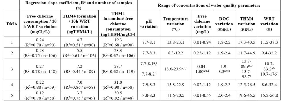
4.3.3 Relationship between free chlorine consumption, THM4 formation and water residence time ... 45
4.3.4 Correlations between water quality parameters across DMAs ... 48
4.3.5 Predictive THM4 approach and validation ... 49
4.4 Discussion ... 50
4.5 Conclusions ... 53
4.6 Acknowledgements ... 54
CHAPTER 5 ARTICLE 2 – ASSESSING THE IMPACT OF DMA IMPLEMENTANTION ON BACTERIAL WATER QUALITY IN A FULL-SCALE DS ... 55
5.1 Introduction ... 56
5.2 Materials and methods ... 58
5.2.1 Characteristics of the DMAs and choice of sampling sites ... 58
5.2.2 Hydraulic network model ... 59
5.2.3 Sampling strategy and analytical methods ... 59
5.2.4 Planktonic bacterial community profiles from inlets, existing and created dead-ends .. 60
5.2.5 Raw HTS data accession number ... 61
5.2.6 Data analysis ... 61
5.3 Results and discussion ... 62
5.3.1 Changes in hydraulic parameter distribution ... 62
5.3.2 Water quality before and after the implementation of DMAs at inlets ... 63
5.3.3 Bacterial water quality changes with DMAs implementation ... 64
5.3.4 Influence of water quality parameters on bacterial variations and community structures across DMAs ... 69
5.4 Conclusions ... 74
5.5 Acknowledgements ... 75
CHAPTER 6 ARTICLE 3 – IDENTIFICATION OF FACTORS AFFECTING BACTERIAL ABUNDANCE AND COMMUNITY STRUCTURES IN A FULL-SCALE DRINKING WATER DISTRIBUTION SYSTEM ... 76
6.1 Introduction ... 78
6.2 Materials and methods ... 79
6.2.1 Water sampling ... 79
6.2.2 Water quality analysis ... 81
6.2.3 DNA extraction and bacterial 16S rRNA gene PCR-amplification and sequencing . 81 6.2.4 Data analysis ... 82
6.2.5 Raw HTS data accession number ... 83
6.3 Results ... 83
6.3.1 Amplification of total bacterial counts and decrease in disinfectant residual concentration through the DWDS ... 83
6.3.2 Bacterial community diversity and composition ... 83
6.3.3 Differences between bacterial communities over time ... 87
6.3.4 Distribution of OTUs across the sub-systems and their relationship with water quality parameters and estimators of diversity and richness ... 88
6.3.5 Opportunist pathogens, cosmopolitan, and endemic species across the specific sub-systems ... 89
6.4 Discussion ... 91
6.5 Acknowledgements ... 96
CHAPTER 7 GENERAL DISCUSSION ... 98
7.1.1 Impact of DMA implementation on hydraulic conditions ... 99
7.1.2 Effects of DMA implementation on water quality ... 100
7.2 Bacterial communities across DWDS ... 104
7.3 Management of DMAs implementation ... 105
7.4 Study limitations ... 106
CHAPTER 8 CONCLUSIONS AND RECOMMENDATIONS... 107
REFERENCES ... 111
LIST OF TABLES
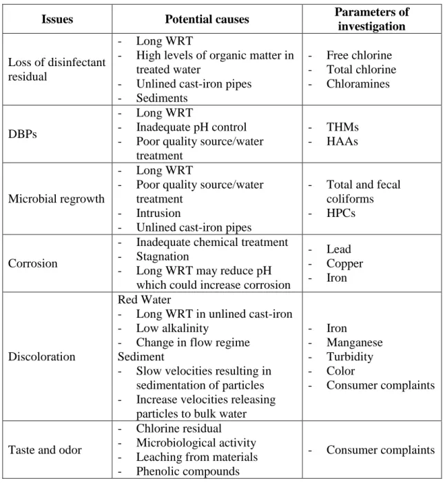
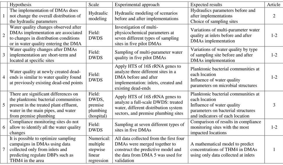
Table 2.1: Water quality issues associated with increased residence time (Source: Brandt, et al. (2004)) ... 17 Table 3.1: DMAs characteristics and sampling frequency ... 26 Table 3.2: Experimental procedure developed to validate (or invalidate) the research hypotheses
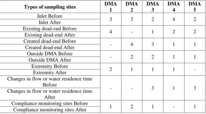
and corresponding articles ... 30 Table 4.1: Number of sampling sites in each DMA by type before and after implementations .... 39 Table 4.2: Correlations between free chlorine consumption, THM4 formation, and water residence
time variations in each DMA ... 47 Table 4.3: Results for the multiple linear regression performed on 169 observations from four
different DMAs to predict THM4 concentrations at a site j from the values measured at an inlet site (i) ... 49 Table 6.1: Number of sequences of indicator species (at genus level) in treated water, distribution
system and taps (α=0.05)... 93 Table A-2.1: Pearson’s correlations between measured water quality parameters in DMAs 1-5 (red
correlations are significant at ρ<0.05) ... 137 Table A-4.1: Pearson’s correlations between measured water quality parameters and log HPC for
each DMA and for all DMAs combined (red correlations are significant at ρ<0.05) ... 148 Table A-4.2: Pearson’s correlations between measured water quality parameters and log total cell
counts for each DMA and for all DMAs combined (red correlations are significant at ρ<0.05) ... 149 Table A-5.1: Characteristics of the samples from premise plumbing ... 151 Table A-5.2: Average estimators of alpha-diversity for treated water (TW), distributed water (DS)
and tap water (TAP) ... 152 Table A-5.3: Frequency of detection of genera containing OPs across the sub-systems ... 153
LIST OF FIGURES
Figure 2.1: Components of leakage and intervention tools (Source: Tardelli Filho (2006)) ... 6
Figure 2.2: Division of a DWDS into DMAs (Source: Farley and Trow (2007)) ... 11
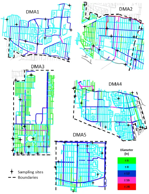
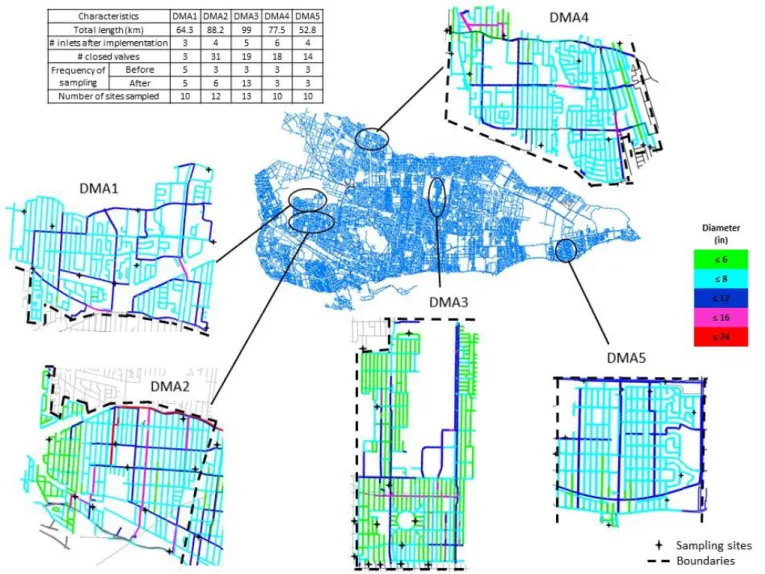
Figure 3.1: DMAs boundaries with pipe diameters and sampling sites locations ... 25
Figure 4.1: DMAs boundaries with pipe diameters and sampling sites locations ... 35
Figure 4.2: Box-and-whisker plots of turbidity and dissolved organic carbon (DOC) across all sampling locations in each DMA. Boxes represent 25th and 75th quartiles of values, whiskers minimum and maximum values and the black squares median values. Before and after groups for each type of site are statistically different at ρ<0.05 by Wald-Wolfowitz Test (*) ... 40
Figure 4.3: Box-and-whisker plots of free chlorine residuals across all sampling locations in each DMA. Boxes represent 25th and 75th quartiles of values, whiskers minimum and maximum values and the black squares median values. Before and after groups for each type of site are statistically different at ρ<0.05 by Wald-Wolfowitz Test (*) ... 41
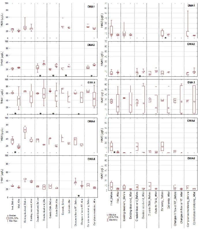
Figure 4.4: Box-and-whisker plots of trihalomethanes (THM4) and haloacetic acids (HAA6) across all sampling locations in each DMA. Boxes represent 25th and 75th quartiles of values, whiskers minimum and maximum values and the black squares median values. Before and after groups for each type of site are statistically different at ρ<0.05 by Wald-Wolfowitz Test (*) ... 42
Figure 4.5: Box-and-whisker plots of total iron (Fe) and manganese (Mn) across all sampling locations in each DMA. Boxes represent 25th and 75th quartiles of values, whiskers minimum and maximum values and the black squares median values. Before and after groups for each type of site are statistically different at ρ<0.05 by Wald-Wolfowitz Test (*) ... 43
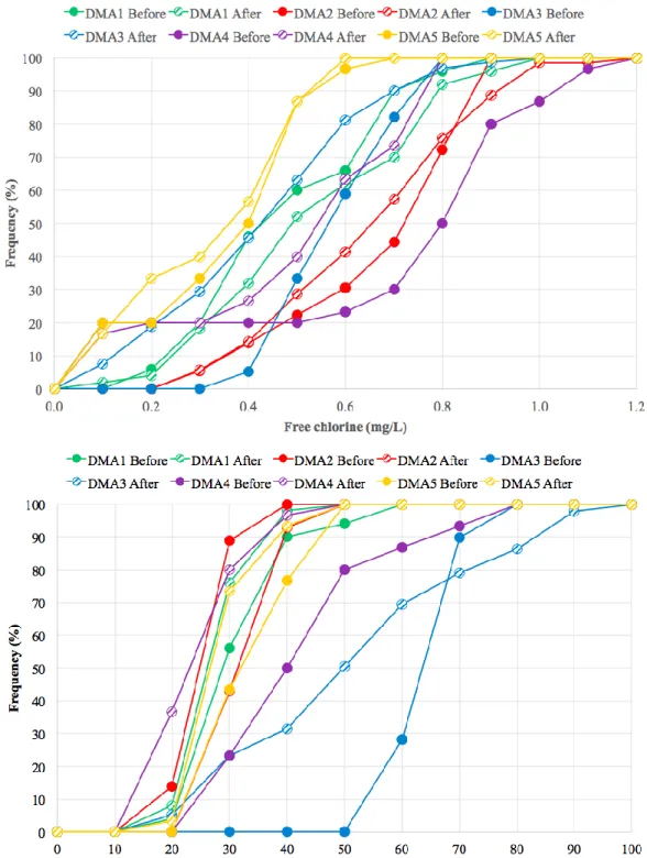
Figure 4.6: Distribution of chlorine residuals and THM4 concentrations at DMAs sampling locations before and after the implementations ... 46
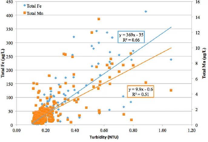
Figure 4.7: Total iron and manganese concentrations versus turbidity values at DMAs1-5 ... 48
Figure 5.1: Overview of the characteristics of DMAs and locations of sampling sites ... 59 Figure 5.2: Mean plots of water quality parameters at inlets in each DMA. Blue lines represent
implementations. Whisker represent 2SD (standard deviation) and the squares mean values. Before and after groups are statistically different at ρ<0.05 by Wald-Wolfowitz Test (*) ... 65 Figure 5.3: Box-and-whisker plots of heterotrophic plate count (HPC) and total bacterial counts
across all sampling locations in each DMA. Boxes represent 25th and 75th quartiles of values, whiskers minimum and maximum values and the black squares median values ... 66 Figure 5.4: Heat map illustrates the relative abundance of different phyla and Proteobacteria classes
in inlets (In), existing dead-ends (Ex), and new created dead-ends (Nw) samples before (Bf) and after (Af) implementations in DMAs 3, 4 and 5. Hierarchical clustering of samples is based on the similarity profile analysis of their bacterial community profiles (significant clusters at α=0.05). Samples with similar community structure cluster together, taking into account the relative abundance of each OTU ... 68 Figure 5.5: Relationship between the logarithm of HPC and total bacteria with the parameters that
have most influenced bacterial changes for all dataset combined (DMAs 1-5) ... 71 Figure 5.6: Dissimilarity in water quality parameters of different types of samples (inlets, existing
and created dead-ends (DE), and other sites) before and after DMAs implementation ... 72 Figure 5.7: Ordination plot of principal component analysis (PCA) showing community
dissimilarities in inlets, existing and new dead-ends (DE) samples before and after implementations for DMAs 3, 4 and 5. The influence of environmental variables (significant variables at ρ<0.1) are presented blue vectors. Axes PC1 and PC2 explained 32% of the variability in the community dissimilarities data ... 73 Figure 6.1: Schematic diagram of the drinking water distribution system sampled illustrating the
sub-systems: treated water (TW), distribution system (DS), and premise plumbing (TAP) . 80 Figure 6.2: Box-plot showing the water quality across the sub-systems (treated water (TW),
distribution system (DS), and premise plumbing (TAP)): (A) free chlorine, (B) water residence time, (C) log of total bacterial counts ... 84 Figure 6.3: Heat map illustrates the relative abundance of different phyla and Proteobacteria classes
in treated water (TW), distribution system (DS) and tap water (TAP) samples. Hierarchical clustering of samples is based on the similarity profile analysis of their bacterial community
profiles (significant clusters at α=0.05). Samples with similar community structure cluster together, taking into account the relative abundance of each OTU ... 85 Figure 6.4: Ordination plot of principal component analysis (PCA) showing distribution of
samples. Samples that cluster more closely together share a greater similarity structure. Axes PC1 and PC2 explained 53% of the variability in the data ... 89 Figure 7.1: Summary of the research conducted ... 98 Figure A-2.1: Box-and-whisker plots of pH and temperature across all sampling locations in each
DMA. Boxes represent 25th and 75th quartiles of values, whiskers minimum and maximum values and the black squares median values ... 133 Figure A-2.2: Box-and-whisker plots of water residence time across all sampling locations in each
DMA. Boxes represent 25th and 75th quartiles of values, whiskers minimum and maximum values and the black squares median values ... 134 Figure A-2.3: Box-and-whisker plots of dissolved iron (Fe) and manganese (Mn) across all
sampling locations in each DMA. Boxes represent 25th and 75th quartiles of values, whiskers minimum and maximum values and the black squares median values ... 135 Figure A-2.4: Predicted THM4_i values vs. observed values from the regression model (A) and
validation of the regression model at DMA 5 using the regression model from DMAs 1-4 (B) ... 136 Figure A-3.1: Décroissance du chlore dans l’eau filtrée de l’usine DesBaillets en avril 2012 à 5° et
20°C ... 141 Figure A-3.2: Cinétique de formation de THM en fonction de la dose de chlore (2 et 3 mg/L avec
et sans ajustement de pH) et de la température (5° et 20°C) ... 142 Figure A-3.3: Formation de THM4 en fonction de la consommation de chlore pour des eaux filtrées
des usines Atwater et DesBaillets. Températures d’incubation de 5° et 20°C avec ajout d’hypochlorites variant de 1,5 à 4 mg/L et des pH ambiants ou fixes à 7,8 ... 143 Figure A-3.4: Évolution du COT à l’eau filtrée de l’usine DesBaillets, 1990-2010 ... 144 Figure A-4.1: Variations in water residence time at minimum demand conditions and maximum
Figure A-4.2: Variations in water velocity at minimum demand conditions and maximum demand conditions ... 147 Figure A-5.1: Venn diagram showing the shared OTUs across the sub-systems ... 154
LIST OF SYMBOLS AND ABBREVIATIONS
ASCE American Society of Civil Engineers APHA American Public Health Association AWWA American Water Works Association
Cl2 Chlorine
CFU Colony forming unit
Cu Copper ions
DBPs Disinfection by-products DMA District metered area DNA Deoxyribonucleic acid DOC Dissolved organic carbon DS Distribution system
DWDS Drinking water distribution system EPA Environmental Protection Agency
Fe Iron
HAAs Haloacetic acids
HPCs Heterotrophic plate counts HTS High-throughput sequencing
in inches
IWA International American Water Association
L Liters
Km Kilometers
m3 Cubic meter
mg Milligrams
mgd Millions of gallons per day min Minutes
Mn Manganese
NRW Nonrevenue water
NSERC Natural Sciences and Engineering Research Council OMBI Ontario Municipal Benchmarking Initiative
OPs Opportunistic pathogens
OPPPs Opportunistic premise plumbing pathogens PVC polyvinyl chloride
rRNA Ribosomal ribonucleic acid spp. Species
THMs Trihalomethanes
UKWIR UK Water Industry Research
USEPA United States Environmental Protection Agency WHO World Health Organization
WRF Water Research Foundation WRT Water residence time
LIST OF APPENDICES
Appendix 1 – Supplemental information: Calibration of hydraulic models ... 128 Appendix 2 – Supplemental information, Article 1: Predicting water quality impact after dmas
implementation in a full-scale dwds ... 132 Appendix 3 – Supplemental information: Formation of THMs at chlorinated treatment plant water ... 138 Appendix 4 – Supplemental information, Article 2: Assessing the impact of DMA implementation
on bacterial water quality in a full-scale DS ... 145 Appendix 5 – Supplemental information, Article 3: Identification of factors affecting bacterial
CHAPTER 1
INTRODUCTION
1.1 Background
Large amounts of treated drinking water carried by distribution systems (15 to 50%) are lost before reaching the customer, not generating any revenue for water utilities (American Water Works Association (AWWA), 2003; Jakubic, 2007; Magini et al., 2007; Smeets et al., 2009). Losses of treated and pressurized water, known as real losses, are comprised of breaks and leaks from water mains and customer service connection pipes, joints, and fittings; from leaking reservoir or tanks walls; and from reservoir or tank overflows (American Water Works Association (AWWA), 2009). The level of these losses depends on the quantity of leaks occurring, their magnitude, the operating pressure, and the duration that the leakage occurs. Furthermore, the volume of losses from many small leaks can surpass that from large reported breaks, since the latter have a run time often limited to a period of hours while small and hidden leaks may last undetected for months or even years (Fanner et al., 2007; Thornton et al., 2008). The World Bank (Kingdom et al., 2006) estimates almost 33 billion m3/year of real water losses worldwide. In addition to being a waste of resources (water and energy), leakage can be a risk to public health caused by external contaminants entering the pipe through leak openings (American Water Works Association (AWWA), 2009).
Maintaining the integrity of drinking water distribution systems (DWDSs) is essential since this is the final barrier before delivery of drinking water to consumers. The principal control tools for breaks and leaks are pressure management and infrastructure replacement (Thornton, et al., 2008). In North America, aging infrastructure is near the end of its useful life (American Society of Civil Engineers (ASCE), 2009) and has been the leading cause of failures and high leakage rates compromising DWDSs efficiency (Ontario Municipal Benchmarking Initiative (OMBI), 2008; American Water Works Association (AWWA), 2009). Nevertheless, since renewal is a very expensive long-term solution, pressure management is a cost-effective way to prevent new leaks in existing aging pipe systems, along active leakage control as well as optimized repairs to extend the life of pipes (Fanner, et al., 2007). Moreover, pressure management reduces flow rates from leakage and new break frequencies and has been successfully used in combination with district metered areas (DMAs) to reduce and identify leaks in DWDSs (Fanner, et al., 2007; American Water Works Association (AWWA), 2009; Kunkel & Sturm, 2011).
DMAs consist in dividing the system into discrete areas, typically from 500 to 3,000 service connections. In this way it is possible to measure flow rates and quantify leakages. However, this practice involves the closing of boundary valves creating dead-ends and hydraulic changes that may result in stagnation, increased water residence time (WRT), and therefore water quality degradation. Factors that can be affected by water residence time and stagnation include several chemical, biological, physical and aesthetic issues such as loss of disinfectant residual (Desjardins et al., 1997; Prévost et al., 1997; Prévost et al., 1998; Baribeau et al., 2001; Rodriguez & Sérodes, 2001; Simard et al., 2011; Machell & Boxall, 2014), disinfection by-products (DBPs) formation (Desjardins, et al., 1997; Speight & Singer, 2005; Rodriguez et al., 2007; Mouly et al., 2010; Simard, et al., 2011), microbial regrowth (Maul et al., 1985; Desjardins, et al., 1997; Prévost, et al., 1997; Prévost, et al., 1998; Carter et al., 2000; Zhang & DiGiano, 2002; Baribeau et al., 2005b; Chauret et al., 2005; Machell & Boxall, 2014), sediment deposition (Gauthier et al., 1999; Barbeau et al., 2005; Vreeburg & Boxall, 2007), corrosion (Eisnor & Gagnon, 2004; Nawrocki et al., 2010), discoloration (Clement et al., 2002; Imran et al., 2005; Vreeburg & Boxall, 2007), and taste and odor problems (Khiari et al., 2002; Maillet et al., 2009).
Despite a number of DMAs implementation being successfully reported by water utilities (UK Water Industry Research (UKWIR), 2000; Fanner, et al., 2007; Kunkel & Sturm, 2011), the published literature presents limited results regarding DMAs impact on water quality from fieldwork studies. Indeed, the limited studies available are either conducted after the implementation, or only once before and after the implementation. As DMA implementation may cause significant changes in the hydraulic parameters that drive water quality, it appeared important to assess the impact of DMA setups on water quality using a comprehensive sampling plan that accounts for changes in distribution operations (WRTs, flow velocities, pressures, etc.) and seasonal variations of incoming water quality (treatment changes, pH, temperature, chlorine residuals, organic matter, metals, bacterial loads, etc.). It also appeared important to expand the water quality parameters considered to provide a better understanding of the source and sanitary significance of any water quality changes.
Consequently, since DMAs implementation is certainly an interesting approach for water utilities to consider, the work outlined in this thesis focused on quantifying the impact of DMAs implementation on water quality by means of a detailed multi-parameter survey on different types of sampling sites during the temporary setup of five pilots sectors in a full-scale DWDS. Such
detailed monitoring constitutes a very significant monitoring commitment and is not feasible outside of a research project scope. In order to assist utilities, we have also developed a sampling approach that can be used combining limited field sampling, hydraulic modeling, and water quality modeling to predict changes in regulatory compliance for DBPs.
1.2 Structure of dissertation
The remainder of this thesis is organized in the following seven chapters. A review on water losses in DWDS, DMAs application and water quality investigations as well as the impact of increasing WRT and hydraulic changes on water quality degradation is provided in Chapter 2. Then, the research objectives, hypotheses and methodology are presented in Chapter 3. Chapters 4 through 6 present our research results in the form of three submitted scientific publications. The first article presents findings from the investigation of the impacts of DMAs implementation on water quality as well as an approach to predict trihalomethanes (THMs) concentrations in DMAs area using parameters measured at an inlet site (Chapter 4, accepted with revisions by Journal AWWA). The following chapter presents findings concerning bacterial changes, including community structures, during DMAs application and association with other water quality parameters (Chapter 5, submitted to Plos One). Chapter 6 reports the results of factors affecting bacterial abundance and community structures along DWDS from treated water to premise plumbing (submitted to Applied and Environmental Microbiology). Finally, a general discussion is provided in Chapter 7 followed by conclusions and recommendations in Chapter 8.
CHAPTER 2
CRITICAL REVIEW OF THE LITERATURE
The purpose of this chapter is to provide a better understanding about real water losses occurring in drinking water distribution systems (DWDSs), the importance and benefits of reducing it as well as presenting the most effective tool commonly used to manage it. This strategy is pressure management associated with the implementation of district metered areas (DMAs). Despite its many benefits, this strategy could increase water residence time (WRT) and the number of stagnant sites in water networks. The published literature is scarce about the impact of increased WRT and the number of dead-ends after DMA implementation. Few studies have been conducted on water quality and can actually quantify the impact of that implementation. They are presented as well as some modeling and historical data analysis studies. Then, the last section presents the potential changes occurring in water quality with time across DWDS.
2.1 Water loss in DWDS
Water loss occurring within DWDS corresponds to the volume of water produced in treatment plants that does not reach the customer, thus not generating revenue for water utilities (American Water Works Association (AWWA), 2009). These losses can be real or apparent losses. Real losses are the physical losses of water comprised of breaks and leaks from water mains and customer service connection pipes, joints, and fittings; from leaking reservoir or tanks walls; and from reservoir or tank overflows. On the other hand, apparent losses are the nonphysical losses that occur when water is delivered to the customer but is not measured or recorded accurately. According to the International Water Association (IWA) and the American Water Works Association (AWWA) water balance methodology, the sum of real and apparent losses plus unbilled authorized consumption is known as nonrevenue water (NRW). The World Bank (Kingdom, et al., 2006) estimates that the worldwide NRW volume amounts to 48.6 billion m3/year (from an annual production of 300 billion m3/year), and from this amount almost 33 billion is due to real losses. In Toronto (Canada), a conservative estimate of 25% represents a loss of more than 120 million m3/year, which could fill more than 50,000 Olympic swimming pools (Jakubic, 2007). In the United States, most states have policies and regulations that limit the maximum acceptable value for water loss within the range of 10% to 15% (United States Environmental Protection Agency (USEPA), 2010). Nevertheless, water loss percentages in the United States can reach more than
30% in some distribution systems (American Water Works Association (AWWA), 2003). The following subsections will focus on the real losses in distribution systems occurred largely due to leakage.
2.1.1 Causes, types and duration of real losses
The most common causes of leakage are pipe age, materials, human error (workmanship defects, poor installation, mishandling of materials prior to installation), environmental conditions (corrosion, weather, vibration and traffic loading) and operational (incorrect backfill, pressure transients, operating pressure, lack of proper scheduled maintenance) (Thornton, et al., 2008). In North America, aging infrastructure is near the end of its useful life (American Society of Civil Engineers (ASCE), 2009) and has been the leading cause of failures compromising system efficiency (Ontario Municipal Benchmarking Initiative (OMBI), 2008; American Water Works Association (AWWA), 2009). The United States utilities needs are estimated at least $11 billion to replace aging facilities that are near the end of their useful life (American Society of Civil Engineers (ASCE), 2009). The cost to renew Ontario’s municipal systems was estimated at $34
billion (Jakubic, 2007). In the City of Toronto, for example, half of the water infrastructure is at least 50 years old and almost 10% dates to over a century.
In a study conducted in 21 Canadian cities, cast-iron pipes were the most susceptible to break, followed by ductile-iron, asbestos-cement, and PVC (Rajani & McDonald, 1995). In Montreal, most breaks were also observed in cast-iron and ductile-iron pipes (Besner et al., 2001). Studies in European countries found that leakage is generally low in networks with high proportion of PVC subjected to low water pressures (Smeets, et al., 2009). LeChevallier et al. (2006) analyzed historical data of leak and repairs verified that most leaks occurred during the winter months and most repairs were performed on small (eight-in) cast-iron pipes that exhibited a circular type of break associated with pipe movement.
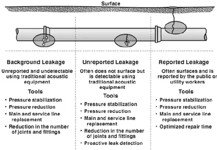
Real losses in pipes can occur as reported, unreported, and background leakage (Thornton, et al., 2008). Figure 2.1 exemplifies the three types and appropriate tools to control them. Reported breaks and leaks are visible and disruptive producing high flow rates being reported to the utility by consumers or utility personnel. Their principal control tools are pressure management and infrastructure replacement. Unreported breaks and leaks are hidden from above ground view producing moderate flow rates being controlled by pressure management and located through
active leak detection. Background leakage corresponds to combined weeps and seeps at joints and on customer service connections presenting typical small flow rates (4 L/min). Also, background leakage is pressure-sensitive and can be addressed by pressure management or infrastructure replacement. However, unlike unreported leakage, background leakage is not detected by conventional acoustic leak detection equipment.
Figure 2.1: Components of leakage and intervention tools (Source: Tardelli Filho (2006))
The level of leakage losses in a distribution system depends on the quantity of leaks occurring, their magnitude, operating pressure, and the total time that the leakage runs (American Water Works Association (AWWA), 2009). Consequently, to contain leakage loss volume it is essential to minimize the duration of individual leaks and to control the operating pressure. The run time of a leak corresponds to three periods: the awareness time (the time it takes for the water utility to become aware that a leak exists), the location time (the time required to locate the leak), and the repair time (the time to conduct repairs of the leak). Furthermore, the volume losses from many small leaks can surpass the volume loss from large reported breaks, since the latter have a run time often limited to a period of hours while small and hidden leaks may go undetected for months or even years (Fanner, et al., 2007; Thornton, et al., 2008).
2.1.2 Reported rates of breaks and leakage losses
Data from water mains breaks in a DWDS shows the occurrence of pipe leaks and are an indicator of infrastructure conditions. A survey conducted by the American Water Works Association (AWWA) (2003) in 337 utilities in the United States and Canada presents an estimate of the mean main break of 13 per 100 Km per year. Another survey including data from 202 utilities from 2003 and 2004, primarily in the United States (2% from Canada), reported higher median values according to utility size: 13.3 breaks per 100 Km per year (<10,000 inhabitants) to 43.8 breaks per 100 Km per year (>500,000 inhabitants) (Lafferty & Lauer, 2005). A similar influence of increased water main breaks as a function of the population size was reported for Quebec cities (Guindon et al., 2008). The break rates per 100 Km per year varied from 7 (municipalities above 3,000 inhabitants) to 44 (municipalities between 50,000 to 100,000 inhabitants). Data from 12 Ontario municipalities show that the city of Toronto, which is the densest city included in that study, has the highest average main break rate: 26 breaks per 100 Km per year (Ontario Municipal Benchmarking Initiative (OMBI), 2008, 2009). However, the city of Windsor with a population of less than 250,000 inhabitants presents the second worst-case value (23 breaks per 100 Km in 2006) among the 12 cities in the report. Average main break rates for the Ontario cities range from 3.9 to 25.8 per 100 Km per year.
The percentage of water loss is widely used to express leakage losses in DWDS. In a typical distribution system 10% of water produced is often lost as leakage (Kirmeyer et al., 2001b) and acceptable values can go up to 15% (American Water Works Association (AWWA), 2003; United States Environmental Protection Agency (USEPA), 2010). However, these losses tend to be larger. A survey conducted by the American Water Works Association (AWWA) (2003) from 35 water utilities in the United States shows loss percentages ranged from 15% to 35%, of which Philadelphia city (the largest population served) showed a loss of 31% and Warren County city (the smallest population served) had a loss of 17%. In Canada, 13 to 40% of treated water is lost before it arrives to the taps in Ontario cities (Jakubic, 2007). In 16 European cities, leakage rates ranged from 3% (in The Netherlands) to 50% (in Bulgaria) (Smeets, et al., 2009). Although the Italian leakage average presented by Smeets, et al. (2009) is 28%, in some cities water losses can be more than 50% (Magini, et al., 2007). It should be noted that in the same distribution system, water losses could vary greatly from one sector to another. As discussed above, the age of the system has great influence on water loss. In the Holy city of Makkah (Saudi Arabia), for example,
field investigations in seven areas have shown variations in water loss ranging from 6% to 56% with an average of 32% (Al-Ghamdi & Gutub, 2002). The old areas of this system, built in 1978-79, showed the highest water loss with an average value of 46%. While the newest areas, built between 1990-94 had an average value of 12%.
2.1.3 Importance and benefits of reduce water loss
The integrity of DWDSs is essential since this is the final barrier before delivery of drinking water to consumers. Leakage can lead to customer inconvenience, damage to infrastructure, excessive costs, increased loading on sewers, introduction of air into the distribution network and risk to public health caused by contaminants entering the pipe through leak openings (Farley, 2001; National Research Council of the National Academies, 2006; American Water Works Association (AWWA), 2009). The distribution system has been identified as the most vulnerable part of the multiple barrier system because of the outbreaks caused by accidental intrusion, as well as its potential for deliberate attacks (Lindley & Buchberger, 2002). The failures in the distribution system can have a contribution around 15% of the overall rate of gastroenteritis in the population (Hunter et al., 2005). However, since many outbreaks are not reported, the true impact of distribution systems in waterborne diseases is estimated to be much higher (Craun et al., 2010). The contamination by intrusion occurs when the pressure surrounding the water main exceeds the internal pressure in the pipe, so the water present external to the pipes may flow in through the leak openings. Studies have shown the effects of pressure transients on distribution system water quality (Kirmeyer et al., 2001a; Karim et al., 2003; LeChevallier et al., 2003; Besner et al., 2008; Besner et al., 2010). Sources of contamination that can potentially intrude into the pipe under favorable conditions include soil, non-potable water, groundwater, and sewage. Pathogens and indicators of fecal contamination have been identified in the environment external to water distribution mains (Kirmeyer, et al., 2001a; Karim, et al., 2003; Besner, et al., 2010).
Moreover, since water demand is increasing and resources are diminishing around the world, the application of available intervention tools is essential in order to optimize water losses in DWDS. The management of water losses has many benefits for the utilities, consumers, and for the environment including reduced costs of captation, treatment, operation, and pumping, increase revenues, water conservation, increased level of service to consumers through increased reliability of supply, improving public perception of water companies (Thornton, et al., 2008).
2.2 Pressure management associated to DMAs as a strategic tool to control and
minimize water losses in DWDS
Real losses in DWDS can be controlled and assessed by implementing an effective leakage management including four key control activities (American Water Works Association (AWWA), 2009):
1. Pipeline and asset management: pipelines eventually reach the end of their useful life and must be rehabilitated or replaced if they are to continue to provide service,
2. Active leakage control: identifying and qualifying existing leakage in a DWDS, typically by performing leak detection surveys and continuous monitoring of flows into small zones or DMAs, 3. Speed and quality of repairs: repairing leaks in a timely and efficient manner,
4. Pressure management: leakage levels can be improved or worsened solely by changes in the level of operating pressure.
Since system renew is very expensive and a long-term endeavor, pressure management is a cost-effective way to prevent new leaks on existing aging pipe systems. Applying active leakage control as well as optimized repairs will extend the life of pipes (Fanner, et al., 2007). Moreover, pressure management reduces flow rates from leakage and new breaks frequencies and has been successfully used in combination with monitored DMAs to reduce and identify leaks (Fanner, et al., 2007; American Water Works Association (AWWA), 2009; Kunkel & Sturm, 2011).
2.2.1 Pressure management
Pressure management in a DWDS involves maintaining pressure at a satisfactory and efficient level avoiding transient pressures and reducing the exceeding pressures, all of which cause unnecessary leaks and breaks (Thornton & Lambert, 2006). This process can be implemented by different tools, including DMAs, pressure sustaining or relief, altitude and level control, transient control and pressure reduction (Fanner, et al., 2007). The benefits of pressure management for leakage control and infrastructure sustainability include the reduction of flow rates from reported and unreported leaks, background leakage, frequency of new breaks, energy costs, inhibition of pressure surges and transients, and extended life of existing infrastructure (Fanner, et al., 2007; American Water
Works Association (AWWA), 2009; Kunkel & Sturm, 2011). Furthermore, the only other way to control background leakage is pipeline rehabilitation/replacement.
Since the rate of leaks or breaks is dependent on the pressure in the system, immediate reduction in the frequency of breaks and leakage has been observed in pressure managed areas in several countries (Lambert, 2000; Thornton & Lambert, 2006). The results after pressure management for 110 sectors from 10 countries shown that the percentage reductions in new breaks (23 to 94%) usually exceeds the percentage reduction in maximum pressure (10 to 75%) (Thornton & Lambert, 2006). The results of DMA implementation and pressure management in the Philadelphia water distribution system showed a significant reduction in leakage and in the 24-hour flow profiles (Kunkel & Sturm, 2011). In this system, leakage has been reduced by 1.19 mgd (from 1.29 to 0.1 mgd) and the 24-hour supply into DMA is about 1.37 mgd less than values before implementation.
2.2.2 District metered areas (DMAs)
DMAs are discrete areas of the distribution system that are sufficiently small (500 – 3,000 customer service connections) to measure and segregate flow rates and quantify leakage events. By limiting supply into the DMA to one or two water mains (Figure 2.2), daily and seasonal variations in flow can be accurately measured by meters placed on the supply mains (Farley & Trow, 2007). The design of a zone for active leakage control has the following aims (Fanner, et al., 2007; American Water Works Association (AWWA), 2009): 1) to divide the system into a number of zones with a defined boundary and appropriately sized. In this way, flows can be monitored and unreported leaks can be distinguished from levels of normal consumption by analyzing flow patterns during minimum consumption; 2) to manage pressure in each zone at the optimum level of pressure, consequently inhibiting the increase of new leaks and removing transients that cause breaks.
Figure 2.2: Division of a DWDS into DMAs (Source: Farley and Trow (2007))
DMA implementation allied with pressure management is an efficient strategy for water utilities willing to employ active leakage control with more accurate measure of water supplied, enabling the identification and quantification of leaks, reduction of pipe breaks, and extension of pipes service life (Thornton, et al., 2008). Moreover, this strategy helps stabilize the network operation, incidents can be contained more easily and their effect will be on a smaller number of consumers (UK Water Industry Research (UKWIR), 2000). However, creating a DMA involves closing boundary valves which create more dead-ends than would normally be found in the system. These locations are known to potentially present stagnation and higher water retention times (WRTs). Additionally, the association with pressure management results in lower water velocities increasing residence times in the sector and consequently the potential for water quality degradation (Brandt et al., 2004; Fanner, et al., 2007; American Water Works Association (AWWA), 2009). Thus, various chemical, biological, physical and aesthetic processes can take place and cause a number of bad side effects in DWDS. These include loss of disinfectant residual, DBPs formation, nitrification, microbial regrowth, sediments deposition, corrosion, discoloration, and taste and odor issues (Smith, 2001; United States Environmental Protection Agency (USEPA), 2002a; Brandt, et al., 2004; National Research Council of the National Academies, 2006). On the other hand, some authors argue that the creation of DMAs allows the water utility to focus more specifically on
valves, fire hydrants, pressure and water quality than in a typical open system (Fanner, et al., 2007; American Water Works Association (AWWA), 2009).
2.3 DMAs application and water quality monitoring
This section presents published literature regarding DMAs implementation and water quality monitoring. Despite sectored areas being prone to have high WRT and more dead-ends, systems that applied this practice have reported no significant changes in water quality supported by scarce data (UK Water Industry Research (UKWIR), 2000; Fanner, et al., 2007; Kunkel & Sturm, 2011). The published literature is insufficient and presents limited results regarding DMAs impact on water quality from fieldwork studies. Despite that, historical data have shown that DMAs could have an impact on discoloration events and higher customer complaints (Armand et al., 2015).
2.3.1 Field cases studies
The effect of DMAs on water quality was investigated by the UKWIR in six DMAs two years after their implementation (UK Water Industry Research (UKWIR), 2000). The objective of this field study was to verify whether there was any difference between water quality measured at locations near the natural system dead-ends (existing before closed valves) and that measured near the boundary valves closed during the DMAs implementation. The water quality parameters verified were chlorine concentrations at 18 locations and particulate matter using ALFI filter paper for a monitoring period of 24 hours at two dead-ends (a new and an old one). A network model was used to determine the WRT at the sampling locations. They found similar chlorine concentrations at both location types in the same DMA and minor differences were attributed to differences in WRT. The filter papers did not show any particulate matter in the water during the sampling at both sites. From these results they concluded that no deterioration in water quality occurred as a result of creating DMAs. Nevertheless, they have not verified the conditions in these sites before the DMAs setup and measurements were conducted only once.
In North America, some water utilities have participated in a project using DMAs as an effective strategy to evaluate and reduce water losses (Fanner, et al., 2007). However, among the participants, only Philadelphia created a DMA by isolating an area from the system and could perform an investigation on water quality before and after the DMA creation. Eldorado and Seattle employed existing pressure control zones for the creation of their DMAs and required no changes
in the zones. In Eldorado, no flushing other than the regular hydrant flushing was performed by the utility as well as no water quality problems were reported over the study period. Halifax’s fully sub-divided network was divided into permanent DMAs prior to the start of the project, and the main focus was to select a zone with appropriate levels of losses to allow detecting results of pressure control. In Halifax, regular flushing was normally performed to meet water quality standards and during the study period no changes in water quality was observed and no complaints were received from the customers inside the DMA. In the Philadelphia network, water quality monitoring was performed prior to the installation of the DMA and after the DMA was in place for several months. They monitored chlorine residuals inside and outside DMA boundaries at 20 fire hydrants, as well as multi-parameters (e.g., pH, heterotrophic plate counts (HPCs), coliforms, and turbidity) testing at three sites within the DMA (two in the central area and one at a distant location from the main inlet). They verified higher chlorine concentrations at most hydrants (17/20). At the three monitoring locations, lower chlorine concentrations were observed when the DMA was in place, but according to the authors, compatible with the levels found in the system in this period. Also, the furthest site presented levels of turbidity above the accepted range after closing valves. They have concluded that the water quality was comparable within the DMA after closing valves and that acceptable water quality should be maintained in this DMA. However, their conclusions were made based on only one measurement before and one measurement after the isolation. Moreover, the comparison was made six months later (November/December vs. May) during different seasons with probably varying water quality conditions and chlorine dosages.
2.3.2 Hydraulic simulations
The UKWIR also investigated the effect of DMAs on water quality using hydraulic simulations in three models covering rural, sub-urban and urban situations (UK Water Industry Research (UKWIR), 2000). They verified the changes in some water quality parameters (chlorine concentrations, WRT, and sedimentation propensity) before and after the implementations with different scenarios relative to number of DMAs and inlets. They observed minor differences at certain sites between the base model and the DMA model. Near the closed valves, residual concentrations and velocities were lower allowing deposition to occur. Elsewhere in the DMAs, chlorine and velocities increased. The overall conclusion was that the introduction of DMAs had no significant effect on water quality on the parameters monitored. However, they verified that as